Representative Selection in Nonmetric Datasets

Abstract

This study considers the problem of representative selection: choosing a subset of data points from a dataset that best represents its overall set of elements. This subset needs to inherently reflect the type of information contained in the entire set, while minimizing redundancy. For such purposes, clustering might seem like a natural approach. However, existing clustering methods are not ideally suited for representative selection, especially when dealing with nonmetric data, in which only a pairwise similarity measure exists. In this article we propose δ-medoids, a novel approach that can be viewed as an extension of the k-medoids algorithm and is specifically suited for sample representative selection from nonmetric data. We empirically validate δ-medoids in two domains: music analysis and motion analysis. We also show some theoretical bounds on the performance of δ-medoids and the hardness of representative selection in general.

View correction statement:

Corrigendum

INTRODUCTION

Consider the task of a teacher who is charged with introducing his class to a large corpus of songs (for instance, popular western music since 1950). In drawing up the syllabus, this teacher will need to select a relatively small set of songs to discuss with his students such that (1) every song in the larger corpus is represented by his selection (in the sense that it is relatively similar to one of the selected songs) and (2) the set of selected songs is small enough to cover in a single semester. This task is an instance of the representative selection problem. Similar challenges often arise in tasks related to data summarization and modeling. For instance, finding a characteristic subset of Facebook profiles out of a large set, or a subset of representative news articles from the entire set of news information gathered during a single day from many different sources.

On its surface, representative selection is quite similar to clustering, a more widely studied problem in unsupervised learning. Clustering is one of the most widespread tools for studying the structure of data. It has seen extensive usage in countless research disciplines. The objective of clustering is to partition a given dataset of samples into subsets so that samples within the same subset are more similar to one another than samples belonging to different subsets. Several surveys of clustering techniques can be found in the literature (Jain, Murty, and Flynn 1999; Xu and Wunsch 2005).

The idea of reducing a full set to a smaller set of representatives has been suggested before in specific contexts, such as clustering xml documents (De Francesca et al. 2003) or dataset editing (Eick, Zeidat, and Vilalta 2004), and more recently in visual (Hadi, Essannouni, and Thami 2006; Chu and Lin 2008) and text summarization (Nenkova and McKeown 2012). It has also been discussed as a general problem in Wang et al. (2013). These recurring notions can be formalized as follows. Given a large set of examples, we seek a minimal subset that is rich enough to encapsulate the entire set, thus achieving two competing criteria—maintaining a representative set as small as possible while satisfying the constraint that all samples are within δ from some representative. In the next subsections we define this problem in more exact terms and motivate the need for such an approach.

Although certainly related, clustering and representative selection are not the same problem. A seemingly good cluster might not necessarily contain a natural single representative, and a seemingly good partitioning might not induce a good set of representatives. For this reason, traditional clustering techniques are not necessarily well suited for representative selection. We expand on this notion in the next sections.

Representative Selection: Problem Definition

Let S be a dataset, be a distance measure (not necessarily a metric), and δ be a distance threshold below which samples are considered sufficiently similar. We are tasked with finding a representative subset that best encapsulates the data. We impose the following two requirements on any algorithm for finding a representative subset:

• Requirement 1: The algorithm must return a subset such that for any sample , there exists a sample satisfying .

• Requirement 2: The algorithm cannot rely on a metric representation of the samples in S.

To compare the quality of different subsets returned by different algorithms, we measure the quality of encapsulation by two criteria:

• Criterion 1: —we seek the smallest possible subset C that satisfies Requirement 1.

• Criterion 2: We would also like the representative set to best fit the data on average. Given representative subsets of equal size, we prefer the one that minimizes the average distance of samples from their respective representatives.

Criteria 1 and 2 are applied on a representative set solution. In addition, we expect the following desiderata for a representative selection algorithm.

• Desideratum 1: We prefer representative selection algorithms that are stable. Let C₁ and C₂ be different representative subsets for dataset S obtained by two different runs of the same algorithm. Stability is defined as the overlap . The higher the expected overlap is, the more stable the algorithm is. This desideratum ensures that the representative set is robust to randomization in data ordering or the choices made by the algorithm.

• Desideratum 2: We would like the algorithm to be efficient and to scale well for large datasets.

Though not crucial for correctness, the first desideratum is useful for consistency and repeatability. We further motivate the reason for Desideratum 1 in Appendix B, and show that it is reasonably attainable.

The representative selection problem is similar to the ϵ-covering number problem in metric spaces (Zhang 2002). The ϵ-covering number measures how many small spherical balls would be needed to completely cover (with overlap) a given space. The main difference is that in our case we also wish the representative set to closely fit the data (Criterion 2). Criteria 1 and 2 are competing goals, because larger representative sets allow for lower average distance. In this article we focus primarily on Criterion 1, using Criterion 2 as a secondary evaluation criterion.

Testbed Applications

Representative selection is useful in many contexts, particularly when the full dataset is either redundant (due to many near-identical samples) or when using all samples is impractical. For instance, given a large document and a satisfactory measure of similarity between sentences, text summarization (Mani and Maybury 1999) could be framed as a representative selection task—obtain a subset of sentences that best captures the nature of the document. Similarly, one could map this problem to extracting “visual words” or representative frames from visual input (Yuan, Wu, and Yang 2007; Mayol and Murray 2005). This work examines two concrete cases in which representatives are needed:

• Music analysis—the last decade has seen a rise in the computational analysis of music databases for music information retrieval (Casey et al. 2008), recommender systems (Lamere 2008), and computational musicology (Cook 2004). A problem of interest in these contexts is to extract short representative musical segments that best represent the overall character of the piece (or piece set). This procedure is in many ways analogous to text summarization.

• Team strategy/behavior analysis—opponent modeling has been discussed in several contexts, including game playing (Billings et al. 1998), real-time agent tracking (Tambe 1995), and general multiagent settings (Carmel and Markovitch 1996). Given a large dataset of recorded behaviors, one may benefit from reducing this large set into a smaller collection of prototypes. In the results section, we consider this problem as a second testbed domain.

What makes both these domains appropriate as testbeds is that they are realistically rich and induce complex, nonmetric distance relations between samples.

The structure of this article is as follows. In the following section we provide a more extensive context to the problem of representative selection and discuss why existing approaches might not be suitable. In

“The δ -Medoids Algorithm,” we introduce δ-medoids, an algorithm specifically designed to tackle the problem as we formally defined it. In “Analysis Summary,” we show some theoretical analysis of the suggested algorithm, and in “Empirical Results” we show its empirical performance in the testbed domains described above. “Summary and Discussion” follow.

BACKGROUND AND RELATED WORK

There are several existing classes of algorithms that solve problems related to representative selection. This section reviews them and discusses the extent to which they are (or are not) applicable to our problem.

Limitations of Traditional Clustering

Given the prevalence of clustering algorithms, it is tempting to solve representative selection by clustering the data and using cluster centers (if they are in the set) as representatives, or the closest point to each center. In some cases it might even seem sufficient, once the data is clustered, to select samples chosen at random from each cluster as representatives. However, such an approach usually considers only the average distance between representatives and samples, and it is unlikely to yield good results with respect to any other requirement, such as minimizing the worst case distance or maintaining the smallest set possible. Moreover, the task of determining the desirable number of clusters k for a sufficient representation can be a difficult challenge in itself.

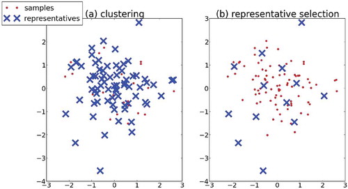
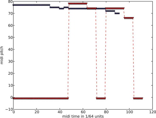
Consider the example in Figure 1: given a set of points and a distance measure (in this case, the Euclidean distance metric), we seek a set of representatives that is within distance 1 of every point in the set, thus satisfying Criterion 1 with . Applying a standard clustering approach on this set, the distance constraint is only consistently met when (and rarely with less than 70 samples). Intuitively, a large number of clusters is required to ensure that no sample is farther than δ from a centroid. However, we can obtain the same coverage goal with only 13 samples. Defining a distance criterion rather than a desired number of clusters has a subtle but crucial impact on the problem definition.

FIGURE 1 Clustering vs. representative selection. (a) When applying k-medoids, k = 77 clusters are required to satisfy the distance condition. (b) A better representative set does so with only 13 representatives.

Clustering and Spatial Representation

The above limitation of clustering applies even when the data can be embedded as coordinates in some n-dimensional vector space. However, in many cases, including our motivating domain of music analysis, the data does not naturally fit in such a space. This constraint renders many common clustering techniques inapplicable, including the canonical k-means (MacQueen et al. 1967), or more recent works such as Wang et al. (2013). Furthermore, the distance function we construct (detecting both local and global similarities) is not a metric, because it violates the triangle inequality. Because of this property, methods reliant on a distance metric are also inapplicable. Among such methods are neighbor-joining (Saitou and Nei 1987), which becomes unreliable when applied on nonmetric data, or the k-prototypes algorithm (Azran and Ghahramani 2006).¹

Nevertheless, certain clustering algorithms still apply, such as the k-medoids algorithm, hierarchical clustering (Sibson 1973), and spectral clustering (Von Luxburg 2007). These methods can be employed directly on a pairwise (symmetric) similarity matrix,² whereas, satisfying the triangle inequality is not a requirement.

The k-Medoids Algorithm

The k-medoids algorithm (Rousseeuw and Kaufman 1990) is a variation on the classic k-means algorithm that selects only centers from the original dataset, and is applicable to data organized as a pairwise distance matrix. The algorithm partitions a set of samples to a predetermined number k based on the distance matrix. Similarly to the k-means algorithm, it does so by starting with k random centers, partitioning the data around them, and iteratively moving the k centers toward the medoids of each cluster (a medoid is defined as ).

All of the approaches mentioned so far are specifically designed for dividing the data into a fixed number of partitions. In contrast, representative selection defines a distance (or coverage) criterion δ, rather than a predetermined number of clusters k. In that respect, k-medoids, or spectral and hierarchical clustering, force us to search for a partition that satisfies this distance criterion. Applying a clustering algorithm to representative selection requires an outer loop to search for an appropriate k, a process that can be quite expensive.

We note that, traditionally, both hierarchical methods and spectral clustering require the full pairwise distance matrix. If the sample set S is large (the usual use case for representative selection), computing a pairwise distance matrix can be prohibitively expensive. In the case of spectral clustering, an efficient algorithm that does not compute the full distance matrix exists (Shu et al. 2011), but it relies on a vector space representation of the data, rendering it inapplicable in our case.³ The algorithm we introduce in this article does not require a distance metric, nor does it rely on such a spatial embedding of the data, which makes it useful even in cases when very little is known about the samples beyond some proximity relation.

Table

Algorithm 1. Extended Greedy K-Centers Approach (farthest first traversal)

1: Input: data sampleSet , required distance δ

2: choose random starting representative

3: representativeSet

4: sampleSet

5: maximalDist

6: while maximalDist > δ do

7:  maximalElement

8:  representativeSet

9:  sampleSet

10:  maximalDist

11: end while

k-Centers Approach

A different, yet related, topic in clustering and graph theory is the k-centers problem. Let the distance between a sample s and a set C be: . The k-centers problem is defined as follows: Given a set S and a number k, find a subset so that is minimal (Hochbaum and Shmoys 1985).

In metric spaces, an efficient two-approximation algorithm for this problem exists as follows.⁴ First choose a random representative. Then, for times, add the element farthest away from the representative set R to R. This approach can be directly extended to suit representative selection—instead of repeating the addition step times, we can continue adding elements to the representative set until no sample is > δ away from any representative (see Algorithm 1).

Although this algorithm produces a legal representative set, it ignores Criterion 2 (average distance).

Another algorithm that is related to this problem is Gonzales’ approximation algorithm for minimizing the maximal cluster diameter (Gonzalez 1985), which iteratively takes elements out of existing clusters to generate new clusters based on the intercluster distance. This algorithm is applicable in our setting because it, too, requires out pairwise distances and can produce a legal coverage by partitioning the data into an increasing number of clusters until the maximal diameter is less than δ (at which point any sample within a cluster covers it). This approach is wasteful for the purpose of representative selection, because it forces a much larger number of representatives than needed.

Finally, in a recent, strongly related study(Elhamifar, Sapiro, and Vidal 2012), the authors consider a similar problem of selecting exemplars in data to speed up learning. They do not pose hard constraints on the maximal distance between exemplars and samples but rather frame this task as an optimization problem, softly associating each sample with a “likelihood to represent” any other sample, and trying to minimize the aggregated coverage distance while also minimizing the norm of the representation likelihood matrix. Though very interesting, it’s difficult to enable this method to guarantee a desired minimal distance, and the soft association of representatives to samples is inadequate for our purposes.

THE δ-MEDOIDS ALGORITHM

In this section, we present the novel δ-medoids algorithm, specifically designed to solve the representative selection problem. The algorithm does not assume a metric or a spatial representation; rather it relies solely on the existence of some (not necessarily symmetric) distance or dissimilarity measure . Similarly to the k-centers solution approach, the δ-medoids approach seeks to directly find samples that sufficiently cover the full dataset. The algorithm does so by iteratively scanning the dataset and adding representatives if they are sufficiently different from the current set. As it scans, the algorithm associates a cluster with each representative, comprising the samples it represents. Then, the algorithm refines the selected list of representatives in order to reduce the average coverage distance. This procedure is repeated until the algorithm reaches convergence. Thus, we address both minimality (Criterion 1) and average-distance considerations (Criterion 2). We show in “Empirical Results” that this algorithm achieves its goal efficiently in two concrete problem domains, and does so directly, without the need to optimize a metaparameter k.

We first introduce a simpler, single-iteration δ-representative selection algorithm on which the full δ-medoids algorithm is based.

Straightforward δ-Representative Selection

Let us consider a more straightforward “one-shot” representative selection algorithm that meets the δ-distance criterion. The algorithm sweeps through the elements of S and collects a new representative each time it observes a sufficiently “new” element. Such an element needs to be > δ away from any previously collected representative. The pseudocode for this algorithm is presented in Algorithm 2.

Table

Algorithm 2. One-shot δ-representatives selection algorithm

1: Input: data , required distance δ

2: Initialize representatives .

3: Initialize clusters

4: representative assignment subroutine, RepAssign, lines 5–22:

5: for i = 0 to m do

6:  Initialize dist

7:  Initialize representative = null

8:  for rep in representatives do

9:   if d(xi, rep) ≤ dist then

10:    representative = rep

11:    dist = d (xi, rep)

12:   end if

13:  end for

14:  if dist ≤ δ then

15:   add xi to clusterrepresentative

16:  else

17:    representative = xi

18:    Initialize clusterrepresentative

19:    add xi to clusterrepresentative

20:    add clusterrepresentative to clusters

21:  end if

22: end for

Although this straightforward approach works well in the sense that it does produce a legal representative set, it is sensitive to scan order, therefore violating the desired stability property. More importantly, it does not address the average distance criterion. For these reasons, we extend this algorithm into an iterative one, a hybrid of sorts between direct representative selection and expectation-maximization (EM) clustering approaches.

The Full δ-Medoids Algorithm

This algorithm is based on the straightforward approach, as described in previously. However, unlike Algorithm 2, it repeatedly iterates through the samples. In each iteration, the algorithm associates each sample to a representative so that it is never away from some representative (the RepAssign subroutine, see Algorithm 3), just as in Algorithm 2. The main difference is that at the end of each iteration it subsequently finds a closer-fitting representative for each cluster S associated with representative s. Concretely, (lines 8–13), under the constraint that no sample ∈ S is farther than δ from medoid_S. This step ensures that a representative is “best-fit” on average to the cluster of samples it represents, without sacrificing coverage. In other words, while trying to minimize the size of the representative set, the algorithm also addresses Criterion 2—average distance as low as possible. This step also drastically improves the stability of the retrieved representative set under different permutations of the data (Desideratum 1). We note that by adding the constraint that new representatives must still cover the clusters from which they were selected, we guarantee that the number of representatives k does not increase after the first scan.

The process is repeated until δ-medoids reaches convergence, or until we reach a representative set which is “good enough” (remember that at the end of each cluster-association iteration we have a set that satisfies the distance criterion). This algorithm uses a greedy heuristic that is indeed ensured to converge to some local optimum (Theorem 1). This local optimum is dependent on the value of δ and the structure of the data. In the later subsection “NP-Hardness of the Representative Selection Problem,” we show that solving the representative selection problem for a given δ is NP-hard, and therefore heuristics are required.

Table

Algorithm 3. The δ-medoid representative selection algorithm.

1: Input: data required distance δ

2: t = 0

3: initialize .

4: initialize

5: repeat

6:

7:  call RepAssign subroutine, lines 5–22 of Algorithm 2

8:  initialize

9:  for cluster in clusters do

10:

11:   add representative to representativest

12:  end for

13: until representativest = representativest–1

Theorem 1. Algorithm 3 converges after a finite number of steps.

See Appendix A for proof sketch.

Merging Close Clusters

Because satisfying the distance constraint with a minimal set of representatives (Criterion 1) is NP-hard (see “Analysis Summary”), the δ-medoids algorithm is not guaranteed to do so. A simple optimization procedure can reduce the number of representatives in certain cases. For instance, in some cases, oversegmentation may ensue. To abate such an occurrence, it is possible to iterate through representative pairs that are no more than δ apart to see whether joining their respective clusters could yield a new representative that covers all the samples in the joined clusters. If it is possible, the two representatives are eliminated in favor of the new joint representative. The process is repeated until no pair in the potential pair list can be merged. This procedure can be generalized for larger representative group sizes, depending on computational tractability. These refinement steps can be taken after each iteration of the algorithm. If the number of representatives is high, however, this approach might be computationally infeasible altogether. Although this procedure was not required in our problem domains (see “Empirical Results”), we believe it could still prove useful in certain cases.

ANALYSIS SUMMARY

In this section, we present the hardness of the representative selection problem, and briefly discuss the efficiency of the δ-medoids algorithm. We show that the problem of finding a minimal representative set is NP-hard and provide certain bounds on the performance of δ-medoids in metric spaces with respect to representative set size and average distance. We continue to show that approximating the representative selection problem is NP-hard in nonmetric spaces, both in terms of the representative set size and with respect to the maximal distance. For the sake of readability, we present full details in Appendix D.

NP-Hardness of the Representative Selection Problem

Theorem 2. Satisfying Criterion 1 (minimal representative set) is NP-Hard.

Bounds on δ-Medoids in Metric Spaces

The δ-medoids algorithm is agnostic to the existence of metric space in which the samples can be embedded. That said, it can work equally well in cases when the data is metric (in Appendix C we demonstrate the performance of the δ-medoids algorithm in a metric space test case). However, we can show that if the measure that generates the pairwise distances is in fact a metric, then certain bounds on performance exist.

Theorem 3. In a metric space, the average distance of a representative set obtained by the δ-medoids algorithm is bound by 2OPT where OPT is the maximal distance obtained by an optimal assignment of k representatives (with respect to maximal distance).

Theorem 4. The size of the representative set returned by the δ-medoids algorithm, k, is bound by where N(x) is the minimal number of representatives required to satisfy distance criterion x.

Hardness of Approximation of Representative Selection in Nonmetric Spaces

In nonmetric spaces, the representative selection problem becomes much harder. We now show that no c-approximation exists for the representative selection problem either with respect to the first criterion (representative set size) or the second criterion (distance—we focus on maximal distance but a similar outcome for average distance is implied).

Theorem 5. No constant-factor approximation exists for the representative selection set problem with respect to representative set size.

Theorem 6. For representative sets of optimal size k⁵ no constant-factor approximation exists with respect to the maximal distance between the optimal representative set and the samples.

Efficiency of δ-Medoids

The actual runtime of the algorithm is largely dependent on the data and the choice of δ. An important observation is that at each iteration, each sample is compared only to the current representative set, and a sample is introduced to the representative set only if it is >δ away from all other representatives. After each iteration, the representatives induce a partition to clusters and only those samples within the same cluster are compared to one another. Whereas, in the worst case the runtime complexity of the algorithm can be , in practice we can get considerably better runtime performance, closer asymptotically to . We note that in each iteration of the algorithm, after the partitioning phase (the RepAssign subroutine in Algorithm 3) the algorithm maintains a legal representative set, so, in practice, we can halt the algorithm well before convergence, depending on need and resources.

EMPIRICAL RESULTS

In this section, we analyze the performance of the δ-medoids algorithm empirically in two problem domains—music analysis and agent movement analysis. We show that δ-medoids does well on Criterion 1 (minimizing the representative set) while obtaining a good solution for Criterion 2 (maintaining a low average distance). We compare our algorithm to three alternative methods—k-medoids, the greedy k-center heuristic, and spectral clustering (using cluster medoids as representatives; Shi and Malik 2000) and show that our algorithm outperforms all three. We note that although these methods weren’t necessarily designed to tackle the representative selection problem, they, and clustering approaches in general, are used for such purposes in practice (see Hadi, Essannouni, and Thami (2006), for instance). To obtain some measure of statistical significance, for each dataset we analyze, we take a random subset of samples and use this subset as input for the representative selection algorithm. We repeat this process N = 20 times, averaging the results and obtaining standard errors. We show that the δ-medoid algorithm produces representative sets at least as compact as those produced by the k-centers approach, but obtains a much lower average distance. We further note it does so directly, without the need for first optimizing the number of clusters k, unlike k-medoids or spectral clustering.

In Appendix C, we also demonstrate the performance of the algorithm in a standard metric space, and show that it outperforms the other methods in this setting as well.

Distance Measures

In both our problem domains, no simple or commonly accepted measure of distance between samples exists. For this reason, we devised a distance function for each setting, based on domain knowledge and experimentation. Feature selection and distance measure optimization are beyond the scope of this work. For completeness, the full details of our distance functions appear in Appendix E. We believe the results are not particularly sensitive to the choice of a specific distance function, but we leave such analysis to future work.

Setting 1—Musical Segments

In this setting, we wish to summarize a set of musical pieces. This domain illustrates many of the motivations listed in the “Introduction.” The need for good representative selection is driven by several tasks, including style characterization, comparing different musical corpora (see Dubnov et al. 2003), and music classification by composer, genre, or period (Bergstra et al. 2006).

For the purpose of this work we used the Music21 corpus, provided in MusicXML format (Cuthbert and Ariza 2010). For simplicity, we focus on the melodic content of the piece, which can be characterized as the variation of pitch (or frequency) over time.

Data

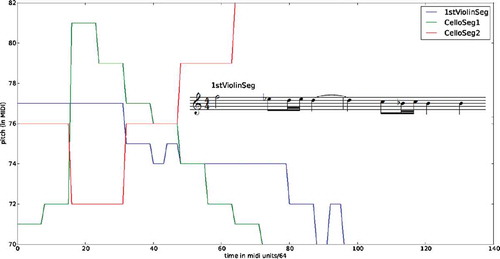
We use 30 musical pieces: 10 representative pieces by Mozart, Beethoven, and Haydn. The melodic lines in the pieces are isolated and segmented using basic grouping principles adapted from Pearce, Müllensiefen, and Wiggins (2008). In the segmentation process, short overlapping melodic sequences 5–8 beats long are generated. For example, three such segments are plotted in Figure 2 as pitch variation over time. For each movement and each instrument, segmentation results in 55–518 segments. All in all, we obtain 20,000–40,000 segments per composer.

FIGURE 2 Three musical segments as pitch (in MIDI format) over time, along with the musical notation of the first segment (1stViolinSeg).

Distance Measure

We devise a fairly complex distance measure between any two musical segments S₁ and S₂. Several factors are taken into account:

• Global alignment—the global alignment score between the two segments, calculated using the Needleman–Wunsch algorithm (Needleman and Wunsch 1970).

• Local alignment—the local alignment score between the two segments, calculated using the Smith–Waterman algorithm (Smith and Waterman 1981). Local alignment is useful if two sequences are different overall but share a meaningful subsequence.

• Rhythmic overlap, interval overlap, step overlap, pitch overlap—the extent to which one-step melodic and rhythmic patterns in the two segments overlap, using a “bag”-like distance function .

The different factors are then weighted and combined. This measure was chosen because similarity between sequences is multifaceted, and the different factors capture different aspects of similarity, such as sharing a general contour (global alignment), a common motif (local alignment), or a similar “musical vocabulary” (the other factors, each of which, by themselves, capture a different aspect of musical language). The result is a measure but not a metric because local alignment may violate the triangle inequality.

Results

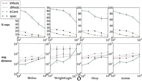
We compare δ-medoids to the k-medoids algorithm and the greedy k-center heuristic for five different δ values. The results are presented in Figure 3. For each composer and δ, we searched exhaustively for the lowest k value for which k-medoids met the distance requirement. We study both the size of the representative set obtained and the average sample-representative distance.

FIGURE 3 Representative set size percentage from entire set and average representative set distance for three different composers, ten different pieces each, and five different distance criteria. Each column represents data for a different composer; δ-medoids yields the most compact representative set overall while still obtaining a smaller average distance than the k-centers heuristic.

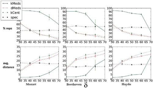
From the representative set size perspective, for all choices of δ, the δ-medoids algorithm obtains better coverage of the data compared to the k-medoids, and does at least as well (and most often better) compared to the greedy k-centers heuristic. However, in terms of average distance, δ-medoids performs much better compared to the k-centers heuristic, implying that the δ-medoids algorithm outperforms the other two. Although spectral clustering seems to satisfy the distance criteria with a small representative set for small values of δ, its noncentroid-based nature makes it less suitable for representative selection, because a more lax δ criterion might not necessarily mean a smaller representative set will be needed (as apparent from the result). Indeed, as the value of δ increases, the δ-medoids algorithm significantly outperforms spectral clustering.

Setting 2—Agent Movement in Robot Soccer Simulation

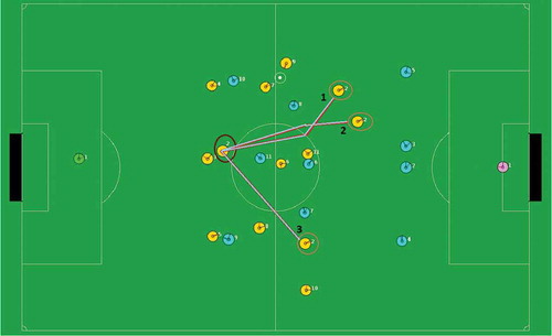
As described earlier, analyzing agent behavior can be of interest in several domains. The robot world-cup soccer competition (RoboCup) is a well-established problem domain for AI in general (Kitano et al. 1997). In this work, we chose to focus on the RoboCup 2D Simulation League. We have collected game data from several full games from the past two Robocup competitions. An example for the gameplay setting and potential movement trajectories can be seen in Figure 4.

FIGURE 4 The RoboCup 2D Simulation. Three potential movement trajectories for a specific agents are marked.

Our purpose is to extract segments that best represent agent movement patterns throughout gameplay. In the specific context of the Robocup simulation league, there are several tasks that motivate representative selection, including agent and team characterization, and learning training trajectories for optimization.

Data

Using simulation log data, we extract the movement of the 22 agents over the course of the game (#timesteps = 6000). The agents move in two-dimensional space (three example trajectories can be seen in Figure 5). We extract 1-second (10 timestamps) long, partially overlapping segments from the full game trajectories of all the agents on the field except the goalkeeper, who tends to move less frequently and in a more confined space and for the purpose of this task is of lesser interest. That leads to 900 · 20 = 18,000 movement segments in total per game. We analyzed four teams and five games (90,000 segments) per team.

FIGURE 5 Representative set size percentage from entire set for four different teams, five different game logs each, and five distance criteria. Each column represents game data for a different team. Axes denoting distance are in log-scale.

Distance Measure

Given two trajectories, one can compare them as contours in two-dimensional space. We take an alignment-based approach, with edit costs being the RMS distance between them. Our distance measure comprises three elements: global and local alignment (same as in music analysis), and a “bag of words”-style distance based on patterns of movement-and-turn sequences (turning is quantized into six angle bins). As in music analysis, the reason for this approach is that similarity in motion is difficult to define, and we believe each feature captures different aspects of similarity. As in the previous setting, this is not a metric, because local alignment could violate the triangle inequality.

Results

As in the previous setting, we compare δ-medoids to the k-medoids algorithm as well as the greedy k-center heuristic, for five different game logs and five different δ values. The results are presented in Figure 5. As before, for each δ, we searched exhaustively for the optimal choice of k in k-medoids. The results reinforce the conclusions reached in the previous domain—for all choices of δ, we meet the distance requirement using a much smaller representative set compared to the k-medoids and spectral clustering approaches (which does much worse in this domain compared to the previous one). Furthermore, δ-medoids once again does at least as well as the k-centers heuristic. In terms of average distance, our algorithm performs much better compared to the k-centers heuristic, suggesting that the δ-medoids algorithm generally outperforms the other approaches.

Stability of the δ-Medoids Algorithm

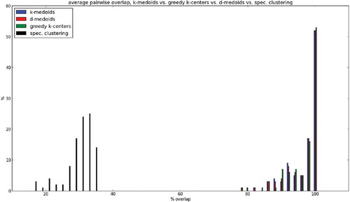
In this section we establish that, indeed, the δ-medoids algorithm is robust with respect to scan order (satisfying Desideratum 1). To test stability, we ran δ-medoids, k-medoids, the k-center heuristic, and spectral clustering multiple times on a large collection of datasets, reshuffling the input order on each iteration, and examined how well preserved the representative set was across iterations and methods. Our analysis indicated that the first three algorithms consistently obtain > 90% average overlap, and the level of stability observed is almost identical. Spectral clustering yields drastically less stable representative sets. For a more complete description of these results see Appendix B.

SUMMARY AND DISCUSSION

In this article, we present a novel heuristic algorithm to solve the representative selection problem: finding the smallest possible representative subset that best fits the data under the constraint that no sample in the data is more than a predetermined parameter δ away from some representative. We introduce the novel δ-medoids algorithm and show that it outperforms other approaches that are concerned only with either best fitting the data into a given number of clusters, or minimizing the maximal distance.

There is a subtle yet significant impact to focusing on a maximal distance criterion δ rather than choosing the number of clusters k. Although both δ-medoids and k-medoids aim to minimize the sum of distances between representatives and the full set, k-medoids does so with no regard to any individual distance. Because of this, we need to increase the value of k drastically in order to guarantee that our distance criterion is met and that sparse regions of our sample set are sufficiently represented. This results in overrepresentation of dense regions in our sample set. By carefully balancing between minimality under the distance constraint and average distance minimization, the δ-medoids algorithm adjusts the representation density adaptively, based on the sample set, without any prior assumptions.

Although this study establishes δ-medoids as a leading algorithm for representative selection, we believe that more sophisticated algorithms can be developed to handle different variations of this problem, putting different emphasis on the minimality requirement for the representative set versus how well the set fits the data. Depending on the specific nature of the task for which the representatives are needed, different trade-offs might be most appropriate and lead to algorithmic variations. For instance, an extension of interest could be to modify the value of δ adaptively, depending of the density of sample neighborhoods. However, we show that δ-medoids is a promising approach to the general problem of efficient representative selection.

FUNDING

This work has taken place in the Learning Agents Research Group (LARG) at the Artificial Intelligence Laboratory, The University of Texas at Austin. LARG research is supported in part by grants from the National Science Foundation (CNS-1330072, CNS-1305287), ONR (21C184-01), AFRL (FA8750-14-1-0070), AFOSR (FA9550-14-1-0087), and Yujin Robot.

Additional information

Funding

This work has taken place in the Learning Agents Research Group (LARG) at the Artificial Intelligence Laboratory, The University of Texas at Austin. LARG research is supported in part by grants from the National Science Foundation (CNS-1330072, CNS-1305287), ONR (21C184-01), AFRL (FA8750-14-1-0070), AFOSR (FA9550-14-1-0087), and Yujin Robot.

Notes

¹ In certain contexts, metric learning (Xing et al. 2002; Davis et al. 2007) can be applied, but current methods are not well suited for data without vector space representation, and in some sense, learning a metric is of lesser interest for representative selection, because we care less about classification or the structural relations latent in the data.

² For spectral clustering, the requirement is actually an affinity (or proximity) matrix.

³ In some cases, the distance matrix can be made sparse via KD-trees and nearest-neighbor approximations, which also require a metric embedding (Chen et al. 2011).

⁴ We note that no better approximation scheme is possible under standard complexity theoretic assumptions (Hochbaum and Shmoys 1985).

⁵ In fact, this proof applies for any value of k that cannot be directly ma nipulated by the algorithm.

⁶ In fact, this proof applies for any value of k that cannot be directly manipulated by the algorithm.

Appendices

A. Proof of Convergence for the δ-Medoids Algorithm

In this section, we show that the full proof that the δ-medoids algorithm converges in finite time.

Theorem 1. Algorithm 3 converges after a finite number of steps.

Proof Sketch: For any sample s let us denote its associated cluster representative at iteration . Let us denote the distance between the sample and its associated cluster representative as . Observe the overall sum of distances from each point to its associated cluster representative, . Assume that after the ith round, we obtain a partition to k clusters, . Our next step is to go over each cluster and reassign a representative sample that minimizes the sum of distances from each point to the representative of that cluster, , under the constraints that all samples within the cluster are still within δ distance of the representative. Because this condition holds prior to the minimization phase, the new representative must still either preserve or reduce the sum of distances within the cluster.

We do this independently for each cluster. If the representatives are unchanged, we have reached convergence and the algorithm stops. Otherwise, the overall sum of distances is diminished. At the (i + 1)–ith round, we reassign clusters for the samples. A sample can either remain within the same cluster or move to a different cluster. If a sample remains in the same cluster, its distance from its associated representative is unchanged. However, if it moves to a different cluster it means that , necessarily, so the overall sum of distances from associated cluster representatives is reduced. Therefore, after each iteration either we reach convergence or the sum of distances is reduced. Because there is a finite number of samples, there is a finite number of distance sums, which implies that the algorithm must converge after a finite number of iterations.

B. Stability of δ-Medoids

In this section we establish that, indeed, the δ-medoids algorithm is robust with respect to scan order (satisfying Desideratum 1 from the “Introduction”). To test this issue, we generated a large collection (N = 1000) of datasets (randomly sampled from randomly generated multimodal distributions). For each dataset in the collection, we ran the algorithm #repetitions = 100 times, each time reshuffling the input order. Next, we calculated the average overlap between any two representative sets generated by this procedure for the same dataset. We then calculated a histogram of average overlap score over all the data inputs. Finally, we compared these stability results to those obtained by the k-medoids algorithm (which randomizes starting positions), the k-centers heuristic (which randomizes the starting node), and spectral clustering (which uses k-means to partition the eigenvectors of the normalized Laplacian). Our analysis indicated that for the first three algorithms, in more than 90% of the generated datasets, there was a > 90% average overlap. The overlaps observed are almost exactly the same, implying that the expected extent of overlap is dependent more on the structure of the data than on the type of randomization the algorithm employs. This serves as evidence that δ-medoids is sufficiently stable, as desired. It should be noted that spectral clustering yields drastically less-stable results (ranging between 15% and 40% overlap), implying a heightened level of stochasticity in the partitioning phase. A histogram indicating our results can be found in Figure 6. One can see that our algorithm has virtually identical stability compared to both k-medoids and the greedy k-center approaches (which, as stated before, are not sensitive to scan order but contain other types of randomization).

FIGURE 6 The histograms (plotted as density functions, i.e., counts normalized as percentages) of the average overlap between representative sets found for each method for the same data under different permutations (overlap measured in %). For k-medoids, δ-medoids, and the k-centers heuristic, in more than 90% of the datasets, there was a > 90% average overlap. Spectral clustering yields drastically less consistent representation sets. The overlaps observed are almost exactly the same, implying that the expected extent of overlap depends more on the structure of the data than on the type of randomization the algorithm employs.

C. Performance of δ-Medoids in Metric Spaces

As we state in the article, though the δ-medoids algorithm is designed to handle nonmetric settings, it can easily be used in metric cases as well. In this section we compare the performance of the algorithm to the benchmark methods used in the “Empirical Results” section. To generate a standard metric setting, we consider a 10-dimensional metric space where samples are drawn from a multivariate Gaussian distribution. We sample a 1000 samples per experiment, 20 experiments per setting, with randomly chosen means and variances. The results are presented in Figure 7.

FIGURE 7 Representative set size percentage from entire set and average representative set distance for four different multivariate Gaussian distributions from which the samples are drawn, 20 different experiments each, and four different distribution values. Each column represents data for a different distribution; δ-medoids yields the most compact representative set overall while still obtaining a smaller average distance than the k-centers heuristic.

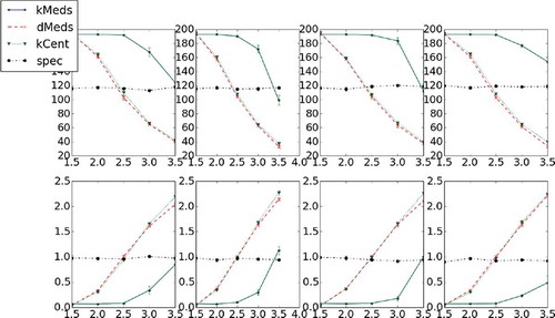
As one might observe, the performance of the δ-medoids algorithm relative to the other methods is qualitatively the same compared to the nonmetric cases, despite the metric property of the data in this setting.

D. Extended Analysis

In this section, we consider the hardness of the representative selection problem, and discuss the efficiency of the δ-medoids algorithm.

D.1 NP-Hardness of the Representative Selection Problem

Theorem 2. Satisfying Criterion 1 (minimal representative set) is NP-Hard.

Proof Sketch: We show this via a reduction from the vertex cover problem. Given a graph we construct a distance matrix M of size . If two different vertices in the graph, , are connected, we set the value of entries (i, j) and (j, i) in M to be . Otherwise, we set the value of the entry to . Formally:

This construction is polynomial in and . Let us assume we know how to obtain the optimal representative set for δ in this case. Then, the representative set S_rep can be easily translated back to a vertex cover for graph G; simply choose all the vertices that correspond to members of the representative set. Every sample i in the sample set induced by M has to be within δ range of some representative j, meaning that there is an equivalent edge , which j covers. Because the representative set is minimal, the vertex set is also guaranteed to be the minimal. Therefore, if we could solve the representative selection problem efficiently, we could also solve the vertex cover problem. Because the vertex cover is known to be NP-hard (Karp 1972), then so is representative selection.

D.2 Bounds on δ-Medoids in Metric Spaces

The δ-medoids algorithm is agnostic to the existence of metric space in which the samples can be embedded. However, we can show that given that the distance measure that generates the pairwise distances is in fact a metric, certain bounds on performance ensue.

Theorem 3. In a metric space, the average distance of a representative set obtained by the δ-medoids algorithm is bound by 2OPT where OPT is the maximal distance obtained by an optimal assignment of k representatives (with respect to maximal distance).

To prove this theorem, and the following one, we will first prove the following helper lemma:

Lemma 1. In a metric space, the maximal distance of a representative set obtained by the one-shot δ-representative algorithm (Algorithm 2) is bound by 2OPT where OPT is the maximal distance obtained by an optimal assignment of k representatives (with respect to maximal distance).

Proof Sketch: Let be the representatives set returned by Algorithm 2. Let a* be the sample, which is the farthest of any points in the representative set, and let that distance be δ*. Consider the set . All points in this set must be of distance > δ* from one another—the algorithm would not select representatives of distance from one another, and , whereas a* is defined as being exactly δ* away from any point in K. Let us consider the optimal assignment of k representatives, K*, and let OPT be the maximal distance it achieves. By the pigeonhole principle, at least two samples in the set must be associated with the same representative. Wlog, let us call these samples x₁ and x₂, and their associated representative. Because the distance between x₁ and x₂ is greater than δ*, and because this is a metric space, by the triangle inequality, the distance of k* from either cannot be smaller than . Therefore .

This implies that Algorithm 2 is asymptotically equivalent to the k-centers farthest-first traversal heuristic with respect to maximal distance.

Now we can prove Theorem 3.

Proof Sketch: First, let us consider Algorithm 2 (one-shot δ-representatives) on which the δ-medoids algorithm is based. By Lemma 1, the maximal distance obtained by it for a representative set of size k is < 2OPT, where OPT is the maximal distance obtained by an optimal solution of size k (with respect to maximal distance). The average distance obtained by Algorithm 2 cannot be greater than the maximal distance, so the same bound holds the average distance as well. Now let us consider the full δ-medoids algorithm—by definition, it can only reduce the average distance (while maintaining the same representative set size). So the average distance obtained by the δ-medoids algorithm must be bound by 2OPT as well.

Theorem 4. The size of the representative set returned by the δ-medoids algorithm, k, is bound by where N(x) is the minimal number of representatives required to satisfy distance criterion x.

Proof Sketch: By Lemma 1, the maximal distance obtained by it for a representative set of size k is < 2OPT, where OPT is the maximal distance obtained by an optimal solution of size k (with respect to maximal distance). Let N(δ) be the covering number for the sample set and distance criterion δ; that is, the smallest number of representative required so that no sample is farther than δ from a representative. The size of the representative set returned by the δ-medoids algorithm, is bound by . Because the full δ-medoids algorithm (Algorithm 3) first runs Algorithm 2 and is guaranteed to never increase the size of the representative set size, the same bound holds for it as well.

In R^d, the covering number is bound by . Given that where K* is the optimal selection of representatives, this implies that the solution returned by δ-medoids is bound by a factor of .

It is equivalent to the similar bound known for the k-center heuristic (Hochbaum and Shmoys 1985, 1986).

D.3 Hardness of Approximation of Representative Selection in Nonmetric Spaces

In nonmetric spaces, the representative selection problem becomes much harder. We now show that no c-approximation exists for the representative selection problem with respect to either the first criterion (representative set size) or the second criterion (distance—we focus on maximal distance but a similar outcome for average distance is implied).

Theorem 5. No constant-factor approximation exists for the representative selection set problem with respect to representative set size.

Proof Sketch: We show this via a reduction from the set cover problem. Given a set of n sets over elements, we construct a graph containing nodes—one node for each subset, and one node for each element. The graph is fully connected . Let and be the sets of nodes for subsets and elements, respectively. We define the distance matrix between elements in the graph (i.e., weights on the edges) to be as follows:

In other words, each node representing a subset is connected to itself and the other subset nodes with an edge of weight 0, and to the respective node of each element it comprises with an edge of weight . Element nodes are connected to all nodes with edges of weight . This construction takes polynomial time. Note that the distance of any element in N (representing subsets) to itself is 0, and the distance of every element in M to itself is . Let us assume we have a c-approximating algorithm for the representative selection problem with respect to representative set size. Any solution obtained by this algorithm with parameter δ would also yield a c-approximation for the set cover problem. Let us observe any result of such an algorithm—it would not return any nodes representing elements (because they are > δ distant from any node in the graph, including themselves). The distance between any nodes representing subsets in the graph is 0, so a single subset node is sufficient to cover all of N. Therefore, the representative set will comprise only elements from N, which directly cover elements in M. An optimal solution for the representative selection algorithm will also serve as an optimal solution for the original set cover problem, and vice versa (otherwise a contradiction ensues). Therefore, a c-approximation (with respect to set size) for the representative selection problem would also mean a c-approxmiation for the set cover problem. However, it is known that no approximation better than clogn is possible (Raz and Safra 1997). Therefore, a c-approximating algorithm for the representative selection problem (with respect to set size) cannot be obtained unless P = NP.

Theorem 6. For representative sets of optimal size k,⁶ no constant-factor approximation exists with respect to the maximal distance between the optimal representative set and the samples.

Proof Sketch: We show this via a reduction from the dominating set problem. Given a graph , a dominating set is defined as a subset so that every node that’s not in V* is adjacent to at least one member of V*. Finding the minimal dominating set is known to be NP-complete (Garey and Johnson 1979).

Assume we are given a graph G and are required to find a minimal dominating set. Let us generate a new graph , where V are the original nodes of G and the graph is fully connected: . The weights on the edges are defined as follows:

This reduction is polynomial. Let us consider an optimal representative set with parameter δ for . Assume it is of size k. This would imply that there’s a dominating set of size k, which is the minimal dominating set obtained in graph G. This dominating set is minimal, otherwise the representative selection set would not be optimal. Let us assume that we have an algorithm for representative selection that’s c-approximating with respect to maximal distance. If there is a dominating set of size k, it would imply a guarantee of on the maximal distance, implying that the algorithm would behave the same as an optimal algorithm (because it cannot use edges of weight ). For this reason, a c-maximum-distance approximation algorithm for the representative selection problem could be used to solve the dominating set problem. Because this problem is NP-hard, it implies no such approximation algorithm exists unless .

D.4 Efficiency of δ-Medoids

The actual runtime of the algorithm is largely dependent on the data and the choice of δ. An important observation is that at each iteration, each sample is compared only to the current representative set, and a sample is introduced to the representative set only if it is > δ away from all other representatives. After each iteration, the representatives induce a partition to clusters and only samples within the same cluster are compared to one another. A poor choice of δ, for instance would cause all the samples to be added to the representative set, resulting in a runtime complexity of . In practice, however, because we compare only from samples to representatives and within clusters, for reasonable cases, we can get considerably better runtime performance. For instance, if the number of representatives is close to , the complexity would be reduced to , which results in a significant speed-up. Again, note that in each iteration of the algorithm, after the partitioning phase (the RepAssign subroutine in Algorithms 2 and 3) the algorithm maintains a legal representative set, so in practice, we can halt the algorithm before convergence, depending on need and resources.

E. Calculating the Distance Measures

In this section we describe in some detail how the distance measures we used were computed, as well as some of the considerations that were involved in their formulation.

E.1 Musical Segments Distance

Segment Information

Every segment is transposed to C. Then, the following information is extracted from each segment:

• Pitch Sequence—the sequential representation of pitch frequency over time.

• Pitch Bag—a “bag” containing all the pitches in the sequence, with sensitivity to registration.

• Pitch Class Bag—a “bag” containing all the pitches in the sequence, without sensitivity to registration.

• Rhythm Bag—a “bag” containing all rhythmic patterns in the sequence. A rhythmic pattern is defined, for simplicity, as pairs of subsequent note durations in the sequence.

• Interval Bag—a “bag” containing all pitch intervals in the sequence.

• Step Bag—a “bag” containing all one-step pitch differences in the sequence; this is similar to intervals, but it is sensitive to direction.

Segment Distance

We devise a fairly complex distance measure between any two musical segments, seg1 and seg2. Several factors are taken into account:

• Global Alignment—the global alignment score between the two segments. This is calculated using the Needleman–Wunsch (Needleman and Wunsch 1970) algorithm.

• Local Alignment—the local alignment score between the two segments. This is calculated using the Smith–Waterman (Smith and Waterman 1981) algorithm.

• Rhythmic Overlap—the extent to which one-step rhythmic patterns in the two segments overlap.

• Interval Overlap—the extent to which one-step interval patterns in the two segments overlap.

• Step Overlap—the extent to which melodic steps in the two segments overlap.

• Pitch Overlap—the extent to which the pitch sets in the two segments overlap. This measure is sensitive to registration.

• Pitch Class Overlap—the extent to which the pitch sets in the two segments overlap. This measure is invariant to registration.

The two alignment measures are combined to a single alignment score. The other measures were also combined to a separate score, which we name the bag distance. The two scores were combined using the l2 norm as follows:

Substitution Function

For both the local alignment and the global alignment, we used a simple exponentially attenuating function based on frequency distance to characterize the likelihood for swaps between any two notes. The function is defined as follows:

The price of introducing gaps was fixed at 1.5.

Bag Distance

To get the bag distance score between two bags we use the calculation

Example

Two example segments are given in Figure 8 in musical notation and in Figure 9 as midi pitch over time.

FIGURE 8 Two segments for example, in musical notation.

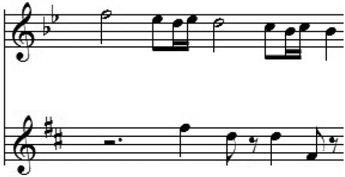
FIGURE 9 Same two segments, plotted as midi pitch over time.

The local alignment distance for these two segments is 0.032. The global alignment distance for these two segments is 1.5. The bag distance score for these two segments is 2.03. The overall combined distance for these two segments after weighting is 20.4.

E.2 Movement Segments Distance

Segment Information

Each segment comprises one agent’s (x, y) coordinates for 10 consecutive timestamps. Then, each segment is translated to start from coordinates (0, 0), and rotated so that, for all segments, all players are facing the same goal. In addition to maintaining the coordinate sequence, from each such segment we extract a bag of movement-turn pairs, where the movement represents distance turns that are quantized into 6 angle bins: forward (−30 to +30 degrees), upper right (+30 to +90 degrees), lower right (+90 to +150 degrees), backward (−150 to +150 degrees), lower left (−90 to −150 degrees), and upper left (−30 to −90 degrees). For instance, the coordinate sequence (0, 0), (0, 10), (5, 10), (8, 14) induces two movement-turn elements: 10+ upper-right turn, 5+ upper-left turn.

Segment Distance

Given two trajectories, one can compare them as contours in two-dimensional space. We take an alignment-based approach, with edit step costs being the RMS distance between them. Our distance measure comprises three elements:

• Global Alignment—The global alignment distance between the two trajectories once initially aligned together (that is, originating from (0, 0) coordinates), calculated by the Needleman–Wunsch algorithm.

• Local Alignment—The local alignment distance between the two trajectories, calculated by the Smith–Waterman Algorithm.

• Movement-Turn bag of words distance—we compare the bag distance of movement-turn elements. We quantize distances into a resolution of 5 meters to account for variation.

• Overall Δ-distance and Δ-angle distance—We also consider the overall similarity of the segments in terms of total distance traveled (and the direction of the movement).

The scores are combined as follows:

Substitution Function

To get the substitution cost for the two alignment algorithms, we simply use the RMS distance between the two coordinates we are comparing. Given two points and , the distance is simply . Gaps were greatly penalized with a penalty of 100 because gaps create discontinuous (and therefore physically impossible) sequences.

Bag Distance

To get the bag distance score between two bags we use the calculation

Example

Two example segments are given in Figure 10.

FIGURE 10 Two movement segments. Each coordinate in the trajectory is labeled with its timestamp in the trajectory . Both segments begin with a long sprint toward one direction and then a sequence of small steps in the opposite direction (scales are × 10).

The local alignment distance for these two segments is 20. The global alignment distance for these two segments is 192.7. The overall delta distance and angle score for these two segments is 61.66 The overall combined distance for these two segments after weighting is 258.72.

REFERENCES

- Azran, A., and Z. Ghahramani. 2006. A new approach to data driven clustering. In Proceedings of the 23rd international conference on machine learning, 57–64. Pittsburgh, PA: ACM.
- Bergstra, J., N. Casagrande, D. Erhan, D. Eck, and B. Kégl. 2006. Aggregate features and ADABOOST for music classification. Machine Learning 65 (2–3):473–84. doi:10.1007/s10994-006-9019-7.
- Billings, D., D. Papp, J. Schaeffer, and D. Szafron. 1998. Opponent modeling in poker. Proceedings of the National Conference on Artificial Intelligence, 493–99. July 26–30, 1998, Madison, WI.
- Carmel, D., and S. Markovitch. 1996. Opponent modeling in multi-agent systems. In Adaption and learning in multi-agent systems, 40–52. Berlin Heidelberg: Springer.
- Casey, M. A., R. Veltkamp, M. Goto, M. Leman, C. Rhodes, and M. Slaney. 2008. Content-based music information retrieval: Current directions and future challenges. Proceedings of the IEEE 96 (4):668–96. doi:10.1109/JPROC.2008.916370.
- Chen, W.-Y., Y. Song, H. Bai, C.-J. Lin, and E. Y. Chang. 2011. Parallel spectral clustering in distributed systems. IEEE Transactions on Pattern Analysis and Machine Intelligence 33 (3):568–86. doi:10.1109/TPAMI.2010.88.
- Chu, W.-T., and C.-H. Lin. 2008. Automatic selection of representative photo and smart thumbnailing using near-duplicate detection. In Proceedings of the 16th ACM international conference on multimedia, 829–32. New York, NY: ACM.
- Clarke, E. and N. Cook. (eds.). 2004. Computational and comparative musicology. In Empirical musicology: Aims, methods, prospects, 103–26. Oxford: Oxford University Press.
- Cuthbert, M. S., and C. Ariza. 2010. Music21: A toolkit for computer-aided musicology and symbolic music data. International Society for Music Information Retrieval Conference (ISMIR 2010). Utrecht, The Netherlands.
- Davis, J. V., B. Kulis, P. Jain, S. Sra, and I. S. Dhillon. 2007. Information-theoretic metric learning. In Proceedings of the 24th international conference on machine learning, 209–16. New York, NY: ACM.
- De Francesca, F., G. Gordano, R. Ortale, and A. Tagarelli. 2003. Distance-based clustering of xml documents. ECML/PKDD 3:75–78.
- Dubnov, S., G. Assayag, O. Lartillot, and G. Bejerano. 2003. Using machine-learning methods for musical style modeling. Computer 36 (10):73–80. doi:10.1109/MC.2003.1236474.
- Eick, C. F., N. Zeidat, and R. Vilalta. 2004. Using representative-based clustering for nearest neighbor dataset editing. Fourth IEEE International Conference on Data Mining, 2004. ICDM’04, 375–78. IEEE. November 1–4, 2004, Brighton, UK.
- Elhamifar, E., G. Sapiro, and R. Vidal. 2012. Finding exemplars from pairwise dissimilarities via simultaneous sparse recovery. In Proceedings of Advances in neural information processing systems, 19–27. December 3–8, 2012, Harrahs and Harveys, Lake Tahoe, CA.
- Garey, M. R., and D. S. Johnson. 1979. Computers and intractability: A guide to the theory of np-completeness. San Francisco, CA: WH Freeman & Co.
- Gonzalez, T. F. 1985. Clustering to minimize the maximum intercluster distance. Theoretical Computer Science 38:293–306. doi:10.1016/0304-3975(85)90224-5.
- Hadi, Y., F. Essannouni, and R. O. H. Thami. 2006. Video summarization by k-medoid clustering. In Proceedings of the 2006 ACM symposium on applied computing, 1400–01. New York, NY: ACM.
- Hochbaum, D. S., and D. B. Shmoys. 1985. A best possible heuristic for the k-center problem. Mathematics of Operations Research 10 (2):180–84. doi:10.1287/moor.10.2.180.
- Hochbaum, D. S., and D. B. Shmoys. 1986. A unified approach to approximation algorithms for bottleneck problems. Journal of the ACM (JACM) 33 (3):533–50. doi:10.1145/5925.5933.
- Jain, A. K., M. N. Murty, and P. J. Flynn. 1999. Data clustering: A review. ACM Computing Surveys (CSUR) 31 (3):264–323. doi:10.1145/331499.331504.
- Karp, R. M. 1972. Reducibility among combinatorial problems. Springer US.
- Kaufman, L. and P. J. Rousseeuw. 1990. Finding groups in data: An introduction to cluster analysis. New York, NY: John Wiley & Sons.
- Kitano, H. et al. 1998. The robocup synthetic agent challenge 97. RoboCup-97: Robot Soccer World Cup I, 62–73. Berlin Heidelberg: Springer.
- Lamere, P. 2008. Social tagging and music information retrieval. Journal of New Music Research 37 (2):101–14. doi:10.1080/09298210802479284.
- MacQueen, J., et al. 1967. Some methods for classification and analysis of multivariate observations. Proceedings of the fifth Berkeley symposium on mathematical statistics and probability, vol. 1, 14. California, USA.
- Mani, I., and M. T. Maybury. 1999. Advances in automatic text summarization. Cambridge, MA: MIT press.
- Mayol, W. W., and D. W. Murray. 2005. Wearable hand activity recognition for event summarization. Proceedings of the Ninth IEEE International Symposium on Wearable Computers, 2005, 122–29. Osaka, Japan: IEEE.
- Needleman, S. B., and C. D. Wunsch. 1970. A general method applicable to the search for similarities in the amino acid sequence of two proteins. Journal of Molecular Biology 48 (3):443–53. doi:10.1016/0022-2836(70)90057-4.
- Nenkova, A., and K. McKeown. 2012. A survey of text summarization techniques. In Mining Text Data, eds. C. C. Aggarwal and C. Zhai, 43–76. Springer US.
- Pearce, M. T., D. Müllensiefen, and G. A. Wiggins. 2008. A comparison of statistical and rule-based models of melodic segmentation. Proceedings of the Ninth International Conference on Music Information Retrieval, 89–94. Philadelphia, PA.
- Raz, R., and S. Safra. 1997. A sub-constant error-probability low-degree test, and a sub-constant error-probability pcp characterization of np. In Proceedings of the twenty-ninth annual ACM symposium on theory of computing, 475–84. New York, NY: ACM.
- Saitou, N., and M. Nei. 1987. The neighbor-joining method: A new method for reconstructing phylogenetic trees. Molecular Biology and Evolution 4 (4):406–25.
- Shi, J., and J. Malik. 2000. Normalized cuts and image segmentation. IEEE Transactions on Pattern Analysis and Machine Intelligence 22 (8):888–905. doi:10.1109/34.868688.
- Shu, L., A. Chen, M. Xiong, and W. Meng. 2011. Efficient spectral neighborhood blocking for entity resolution. In 2011 IEEE 27th international conference on data engineering (ICDE), 1067–78. IEEE.
- Sibson, R. 1973. Slink: An optimally efficient algorithm for the single-link cluster method. The Computer Journal 16 (1):30–34. doi:10.1093/comjnl/16.1.30.
- Smith, T. F., and M. S. Waterman. 1981. Identification of common molecular subsequences. Journal of Molecular Biology 147 (1):195–97 . doi:10.1016/0022-2836(81)90087-5.
- Tambe, M. 1995. Recursive Agent and Agent-Group Tracking in a Real-Time Dynamic Environment. Proceedings of the First International Conference on Multiagent Systems, June 12–14, 1995, San Francisco, California, USA.
- Von Luxburg, U. 2007. A tutorial on spectral clustering. Statistics and Computing 17 (4):395–416. doi:10.1007/s11222-007-9033-z.
- Wang, Y., S. Tang, F. Liang, Y. Zhang, and J. Li. 2013. Beyond kmedoids: Sparse model based medoids algorithm for representative selection. In Advances in multimedia modeling, 239–50. Berlin Heidelberg: Springer.
- Xing, E. P., A. Y. Ng, M. I. Jordan, and S. Russell. 2002. Distance metric learning, with application to clustering with side-information. Advances in Neural Information Processing Systems 15:505–12.
- Xu, R., and D. Wunsch. 2005. Survey of clustering algorithms. IEEE Transactions on Neural Networks 16 (3):645–78. doi:10.1109/TNN.2005.845141.
- Yuan, J., Y. Wu, and M. Yang. 2007. Discovery of collocation patterns: From visual words to visual phrases. In IEEE conference on computer vision and pattern recognition, 2007. CVPR’07, 1–8. IEEE.
- Zhang, T. 2002. Covering number bounds of certain regularized linear function classes. The Journal of Machine Learning Research 2:527–50.