Turnover Prediction in a Call Center: Behavioral Evidence of Loss Aversion using Random Forest and Naïve Bayes Algorithms

Abstract

It is well known that call centers suffer from high levels of employee turnover; however, call centers are services that have excellent operational records of telemarketing activities performed by each employee. With this information, we propose to use the Random Forest and the naïve Bayes algorithms to build classifiers and predict turnover of the sales agents. The results of 2407 sales agents’ operational performance records showed that, although the naïve Bayes is much simpler than Random Forest, both classifiers performed similarly, achieving interesting accuracy rates in turnover prediction. Moreover, evidence was found that incorporating performance differences over time increases significantly the accuracy of the predictive models up to 85%, with the naïve Bayes being quite competitive with the Random Forest classifier when the amount of information is increased. The results obtained in this study could be useful for management decision-making to monitor and identify potential turnover due to poor performance, and therefore, to take a preventive action.

INTRODUCTION

A recurrent problem for call centers is the high turnover rate of the employees. High turnover implies high promotional costs to capture new employees, high recruiting costs, and costs associated with ongoing training and induction of new sales agents. Additionally, personnel and human resources are forced to endure high workloads to meet the constant requirements of applications to fill vacant jobs.

Call centers are becoming increasingly important to business success. Companies have been incorporating, internally or externally, call centers to support their business units in order to establish a platform for continuous contact with the customer. In Chile, the call centers industry during 2012 generated sales over US $400 million, of which US $350 million apply only to outsourcing services; and it could grow between 4% and 5% because of the extension of the offer and the degree of professionalization (Diario Financiero 2012). This reflects the extensive use of subcontracting and employing part-time workers as strategies to increase productivity and organizational flexibility. However, there are some problems with regard to competitiveness because many telemarketing operations are moving to countries such as Peru and Colombia, where labor is less expensive. In Chile, the average pay per working hour for a call center operator is US $4.82, whereas in Colombia and Peru it is US $1.03 and US $1.10, respectively (Concha 2010). However, a way to compete with these lower costs is through further development of human capital through training and specialization. The staff of a call center is relatively young for the entire segment of call center workers, representing 80% of the total workers in each firm, a trend that has continued over time (Diario Financiero 2012). This is a trend that characterizes the call centers worldwide. Twenty-two percent of the call centers, which is considered to be a low-skilled job, recruit people with a college degree (Holman, Batt and Holtgrewe 2007).

Because the work of the operators in a call center involves interacting with people, they must have psychological and personality characteristics that enable them to function in an atmosphere of constant hostility and rejection (Sawyerr et al. 2009). A call center is a system designed to link an agent with a client or potential client on behalf of the firm. In both cases, the agent must possess the skills required to interact with people, whether for reception of information such as queries, complaints, or to transmit information such as description and sales of products and services. Because the agent’s job involves interacting with people, the agents must show certain characteristics that enable them to function effectively in an atmosphere of constant hostility and rejection. This is especially important for agents that operate in outbound call centers. High stress, persistent refusal, direct supervision, and monotony can frustrate the agent and start a process of turnover. Outbound campaigns typically try to maximize the volume of calls, and therefore, cause fatigue for the employee and some corporate image damage because of the repetitive nature of the calls. The emotional burnout also plays an important role. Customer complaints and repeated denials of customers to accept an offer may influence an agent’s motivation (Wallace, Eagleson and Waldersee 2000). For this type of job, personality characteristics are needed that allow the agent to have a strong resilience and tolerance to rejection. The call center agent constantly performs emotional labor to maintain physical and emotional stability by suppressing emotions induced by others (Taylor and Bain 1999; Hoschschild 1983).

The application of data mining techniques to the problem described could assist in discovering patterns in the data of operational activities of the sales campaigns. These patterns can help in decision-making with regard to the necessary assistance to the sales agents by the organization to improve their performance, or early detection of the agents who do not possess the skills needed for the job.

The call centers are unique examples of services that are characterized by excellent operational records of telemarketing activities performed by each employee. This makes it possible to access databases with sufficient detail to find recurring patterns to detect possible cases of voluntary resignations. Valle, Varas and Ruz (2012), trained a naïve Bayesian network to predict the performance of sales agents in a call center and found satisfactory results. However, the study did not address the issue of employee turnover directly, but indirectly through the income that the agents garnered in a given period. In this study, we take a step forward in formulating a model to predict the turnover directly. A sample of the operating performance of the sales agents of an outbound call center dedicated to the sales of insurances was taken. From this sample, a database was obtained with operating results recorded during the recruiting and hiring process of the sales agents, including performance variables describing activity and daily operation of the agents in their jobs. With this data, two classifiers, the Random Forest algorithm (RF) and the naïve Bayes (NB) were trained and analyzed for their ability to predict the rotation of agents in a given time period.

The remainder of this article is organized as follows: in the following section, we review the current system of selection of the sales agents in the call center. “Methodology and Data Management” explains the methodology and data manipulation. The section after that gives a brief description of Random Forests, naïve Bayes, and the turnover prediction problem. A classification approach to solve this problem is presented in “Classifier Construction”, followed by the “Results.” “Practical Application” describes an application example using the best trained classifier. Conclusions are given in the final section.

CURRENT SYSTEM OF RECRUITMENT AND SELECTION OF SALES AGENTS

The recruitment and selection process of a call center located in Santiago, Chile, begins with the announcement in the media of the availability of jobs for telemarketing sales agents. On the basis of these ads on the Internet and in the local newspapers, the candidates are invited for a meeting on a specific day and time. On the basis of those meetings, there are personal and group interviews wherein the selection department assess personal information of the individual, mainly socioeconomic data and income expectations. After those interviews, the department performs a selection of applicants for the job.

The selection is often subjective. The interviewer pays special attention to diction and work experience of the applicant. Selected applicants are assigned to campaigns that have vacancies and they begin an induction course directed by the supervisor of the campaign. This induction course does not last more than five days. At this stage, the call center starts recording the operational activity of the agent. This information is recorded every day. This makes it possible to obtain longitudinal datasets of each operator working from the start of his workday to the month in which he ceases to operate. After the induction course, sales agents continue to perform in the campaign for at least two months.

To ensure the hiring of sales agents with a certain level of skill for the job, the call center has a two-stage insertion: the sales agent has a one-month trial. After this first month of work, the call center evaluates his/her performance and decides whether the individual will continue for a second-month trial. Otherwise, there is an involuntary turnover. After the end of the second month of work, the call center reevaluates the agent’s performance and determines whether he or she is hired, otherwise, there is a voluntary or involuntary turnover. That is, if the subject achieved acceptable performance for two consecutive months, the agent is hired indefinitely. However, this system does not ensure that there will be a voluntary turnover in subsequent months. In fact, 75% of severances (voluntary and involuntary) occur in the first month of work. This system tries to hire only those individuals who have the skills for this job that allow them to perform reasonably well for as long as possible.

The system of recruitment and selection is quite basic and has not developed systematic procedures to acquire subject information on job expectations, personality, or behavior elements to verify a fit between the job and the person.

The recruitment model can be represented by the following notation: let be the performance attributes of the sales agent in the period . Let be the class variable indicating the state of activity of agent in the call center. If there is no activity (i.e., no logged hours) of the agent in the period , then , which is interpreted as a quit. Otherwise, . The goal of the classifier is to predict the class variable (i.e., whether the agent will work in the period j) given operational performance results . Obviously, under this scheme, it is not possible to predict . The unit of measurement of time in our model is months because the recruiting system is designed on the basis of the information that is analyzed at the end of each working month for each agent.

METHODOLOGY AND DATA MANAGEMENT

A sample of 3543 records of performance and sales activity of agents dedicated to 91 sales campaigns of insurances against theft, fraud, fire, disease, and some few campaigns of sales of cell phone plans were taken. This sample represents the call center activity between May 2010 and November 2011. This period covers more than one year of a normal operation.

Operational performance data of sales agents engaged in insurance sales campaigns were used. In this study, we understand operational performance as a set of variables measuring the agent’s activities while working in the call center. These are

1. Logged hours: Includes date and time of starting and ending of a workday. It represents the working hours of the agent logged on to the computer system in his work station.

2. Talked hours: Represents the amount of time the agent is talking directly to a client trying to sell the product and it reflects the effort that the agent dedicates to meet production targets.

3. Effective contacts: Represents the events in which the agent is able to establish a telephone contact with the customer identified in the database of the call center. A sale is not possible without an actual contact. For example, an agent with a high proportion between approved sales and effective contacts is an indicator of the ability to sell the product.

4. Number of approved sales: Represents the output during a given period. From approved sales, the agent earns his salary. It is worth mentioning at this point that the revenues depend only on approved sales plus a minimum income, which is subject to the current legislation. Thus, the operator is subject to high variability or uncertainty in his income because the salary is based only on performance.

5. Number of finished records: A record is finished when the client explicitly states that he or she does not want the product. In this case, the agent closes the record and cannot reconnect with the client via telephone. For example, an agent with a high level of finished records but low level of approved sales represents an inexperienced agent who has difficulties in closing the deal with the customer.

6. Approved production: Represents the monetary value equivalent to the approved sales, further including, incentives and bonuses that the agent received as part of the remuneration policies of the call center.

The information source comes from the automatic log sales activity. This system records all the agent’s activities from the moment he/she begins the workday until the end. The dataset was created from SQL-stored queries. Each record includes the results of each of the six variables described per month from the first month of work to the last, including the campaigns in which the agent participated. In this sample, three records were removed because they had approved sales greater than zero and zero hours spoken. Additionally, we identified 1040 records corresponding to agents who entered the call center but their production was nil, and they were subsequently dismissed from the organization (they worked in the call center only one week or less). Other sales agents are able to stay longer and develop a long or medium-term relationship with the call center. These people are able to develop a better and more steady performance. For example, we observed that only 29% of the agents stayed more than two months in this work. The remaining were subjected to involuntary or voluntary turnover because of poor performance. The resulting sample was 2407 records.

Because there are a variety of sales campaigns, different kinds of insurance, and different working hours (full time and part time¹), a fair comparison is necessary between different types of workdays among different campaigns. For this reason, each performance attribute is divided by the total sum of logged hours in the period of analysis. For example, for a turnover prediction at the third month, , the sum takes into consideration the performance of the first two months and then divides by the logged hours of the first two months of work. Approved sales, finished records, and effective contacts have a highly skewed distribution to the right, which escapes the assumptions of normality. This is a common characteristic of pay-for-performance systems, in which very few obtain outstanding sales levels, whereas most agents have low operational performance or low sales levels. All the variables have been standardized (Steinley 2004). Next, RF and NB classifiers were designed and trained to discriminate between subjects that will continue working or not continue working in the call center, on the basis of their past performance attributes.

RANDOM FOREST, NAÏVE BAYES AND THE TURNOVER PREDICTION PROBLEM

The RF (Breiman 2001) is a supervised classification technique based on classification trees (Breiman et al. 1984). The algorithm consists in learning a set of weak learners. In the case of RF, weak learners are decision trees. We have a set of training data ), , where is a input vector of operational performance of the agents, and is the class variable or the predictor output. A predictor is a weak learner with low bias and high variance (Breiman 2004). The RF algorithm performs a random sampling with replacement from the set , and a set of learners is created, where is the random vector of data selected on the kth tree. The remaining samples are the out-of-bag (OOB) samples, which are then used to evaluate the performance of the RF. The trees are built by a recursive partitioning algorithm and with a random sample of predictors for each one, which allows a low correlation between trees and prevents overtraining. The OOB is used as a testing sample. Each record in this sample is classified in each of the trees in the forest and then determines the class to which the instance belongs according to the resulting unweighted class majority. Using a combination of trees rather than just one generates a classifier that is robust with respect to outliers and noise.

An interesting feature of RF is the possibility to compute the degree of importance of the attributes in the class prediction (Verikas, Gelzinis, and Bacauskiene 2011). RF provides an index of importance for each of the attributes used in the classification task, which indicates the predictive power that has that attribute as a discriminator between different classes. It is computed through the error rate (Breiman 2001). The idea is that, after the trees are built, the values of the variable are permuted randomly in the OOB data and a classification task is run for each instance. Then the error rate is computed. This procedure is repeated for the M variables. Then M error rates are computed. The largest error rate associated to the variable means a greater importance of that attribute to establish association rules and improve the predictive power. In the opposite case, if the increase in the error rate is low, relative to other attributes, then the level of importance of the attribute is lower.

In this study, the operational performance of the sales agents of the call center is characterized by just a handful of attributes. For this reason we do not use preselected attributes, but we use all the information available. This is unlike what occurs, for example, in the study by Hardman, Paucar-Caceres, and Fielding (2013), which combines several databases, resulting in a significant number of attributes available for analyzing student progression through RF.

We compare the performance of RF with a very simple classifier, the naïve Bayes (NB) (Duda and Hart 1973). The NB classifier follows the Bayes formula:

(1)

The NB makes a strong independence assumption among its attributes, assuming that all the attributes are conditionally independent given the classification variable. Thus, under the assumption that the occurrence of a particular value , given that we have a class , we can model as

(2)

The NB can also be seen as a Bayesian network classifier (Ruz and Pham 2009). Essentially, this model tries to find the class value, for each example, that maximizes the posterior probability (the probability of a class value, given a set of attributes) using the Bayes rule. We will see that, for this application, the independence assumption is not always true. Nevertheless, results will show that the performance of this classifier is quite competitive when compared to RF.

NB and RF have been used for a variety of industrial applications. For example, in medical applications (Wiggins et al. 2008), in mechanical applications (Muralidharan and Sugumaran 2012), in imagery applications (Tahir et al. 2013). However, in employee turnover problems, there are fewer examples of applications of data mining to address this problem.

A novel aspect of this study is that we propose that the operational attributes contain information not only as a final result of the sales activities in a given period for a given agent, but that they also contain behavioral information, because the subject keeps in memory the past results, and therefore, that last information must also influence the future decision to continue participating in the call center. For example, a poor sales result in the second month compared with an outstanding result in the first could raise doubts in the subject about the permanence in this job. To capture this effect, we suggest the use of differences in performance over time.

The idea of taking differences over time on performance results, comes from the concept of reference points. Absolute values and references from past outcomes are elements that subjects take into consideration to make a decision. This explanation is the spirit of the Prospect Theory of Kahneman and Tversky (1979) and Tversky and Kahneman (1991). People have a strong loss aversion, which is measured relative to a reference point. That is, people are more sensitive to income changes under the reference point (i.e., losses) than over that reference (i.e., gains).

We conjecture that the operational results of the first month of work (particularly approved sales and approved production) serve as a reference point against which to evaluate performance during the second period of work. Under Prospect Theory, a loss (i.e., a decrease in revenues or sales compared to the first month of work), negatively impacts job satisfaction (Shahnawaz and Jafri 2009; Cotton and Tuttle 1986), which in turn increases the possibility of withdrawal intentions. However, the impact of a profit or revenue performance above the reference is less significant (in absolute terms) than an equivalent loss, but the possibilities of increasing the intentions of resignation are minimal. We presume that approved sales and production of the sales agents in a given period are key variables in job satisfaction, because from them follows income. For this reason, we incorporate as predictor variables the difference between the approved sales in month and ; similarly, for the production attribute.

When there is no reference point made by previous experience, as is the case of the first month of work, the agent might anyway have a reference point corresponding to a minimum acceptable income from other job experiences; so in this case, the reference is exogenous. We have no access to this information, therefore, it is not possible to construct an attribute with the difference (positive or negative) relative to this initial reference point. For this case (i.e., the first period of work), we have only operational information.

CLASSIFIER CONSTRUCTION

For the classifier design effects, there are two classes: those who leave the call center and those who continue working, in a period of time. Each agent is characterized by a set of attributes. It is expected that these attributes can predict the class variable, indicating whether an agent belongs to one class or the other. The objective is to train an RF and NB capable of classifying automatically each instance (agent).

Six operational variables were taken for each agent. The variables were divided by the sum of logged hours in the period of interest and were standardized. The class variable was defined as

(3)

where is logged hours of the ith individual in the jth month. This variable represents the active or inactive state of the operator at the end of the period. The classifier will use all the information available until the j − 1th month.

To visualize the predictive power of the operational variables on the variable performance class, we performed a principal component analysis (PCA) over the set of five operational attributes. The analysis revealed that the first two components explain 61% of the variability of the data. Figure 1 shows a projection of the predictor variables coloring each instance according to the class to which it belongs. This was done using operational information from agents with two months of work. It is possible to distinguish a certain degree of overlapping between both classes. Subjects with turnover in the third month are represented by symbols, whereas subjects that are still working are represented by o symbols.

FIGURE 1 A principal component analysis projection of the first two months of the operational performance of the sales agents.

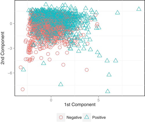
The ideal case is when both distributions (class 1 and class 0) are well separated from each other, which is indicative that the attributes have good discrimination power. However, as Figure 1 shows, there is overlapping between the distributions, which is indicative of the difficulties that the classifier will confront.

RESULTS

In order to see the application of the RF and NB classifier, we took the operational data of the 2407 sales agents of the call center.

The first dataset considered only two months of work in order to predict turnover in the third month (j = 3). This case is of practical interest to the call center because of the recruitment and selection system described earlier. The human resource manager wants to know as soon as possible the potential permanence of an operator (which is subject to performance evaluations and productivity) in order to determine if the operator is eligible to continue for a third month of work (and move to a permanent contract) or subject to a separation before this period. The second dataset considered only one month of work to predict turnover in the second month (j = 2). This allows us to observe the effect on the performance of the classifier when we advance the time of the prediction. The results of the training and testing using 10-fold cross validation of an RF and an NB classifier are shown in Table 1. In 10-fold cross validation (Witten, Frank, and Hall 2011), the original dataset is randomly partitioned in ten equally sized groups: nine partitions are used to train the classifier, and the remaining partition is used for testing. This process is repeated ten times so that each partition is used as a test set once. The correct classification result, on the test set, of each process is averaged to obtain a final estimation of the performance of the classifier. The performance measures are derived from the confusion matrix of each of the test sets.

TABLE 1 Results of RF and NB Classifiers for Predicting Turnover at the Third Month Using a 10-Fold Cross Validation

		Using Raw Attributes				Using Raw Attributes Plus Differences
		RF		NB^a		RF		NB^a
		Mean	SD	Mean	SD	Mean	SD	Mean	SD
CV	Recall	.723	.0239	.779	.0429	.837	.0344	.833	.0305
	Precision	.630	.0347	.780	.0377	.813	.0485	.867	.0235
	Accuracy	.745	.0131	.742	.0293	.856	.0249	.828	.0239
	AUC	.999	0	.812	.0316	1	0	.911	.0154
OOB	Recall	.736	.0058	–	–	.834	.0053	–	–
	Precision	.636	.0056	–	–	.816	.0063	–	–
	Accuracy	.753	.0036	–	–	.856	.0037	–	–

Note: Accuracy was computed as: (true positive + true negative)/N; Precision was computed as: true positive/(true positive + false positive); Recall was computed as: true positive/(true positive + false negative).

^a Since the predictor variables are all continuous, a supervised discretization (Fayyad and Irani 1993) was done for the naïve Bayes classifier. Also, a naïve Bayes classifier was tested without discretization, using Gaussian distributions for each predictor variable. The performance was slightly inferior to the discretized version.

The results in Table 1 show different performance measures computed from the confusion matrix (Witten, Frank, and Hall 2011). We have computed the averages and standard deviations of accuracy, recall, precision, and the area under the curve (AUC) for RF and NB classifiers using only operational attributes, and then afterward, operational attributes plus temporal differences. For a fair comparison of performances between the classifiers, we also report the results of a 10-fold cross validation of the RF classifier.

It can be seen from Table 1 that the RF performance measures are over 70% percent, except for the precision, indicating that the classifier is having weaknesses with the false positive rates.

When compared to the NB, it is observed (cross-validation results) that the performance measures are all above the 70% outperforming the RF, but not to the extent of AUC. Both classifiers have virtually identical accuracy. The accuracy of the RF and the NB using operational attributes did not differ t(9) = .30, p = .39. It appears that NB is a respectable competitor of RF in this problem, although the attributes in our datasets do not satisfy the independence assumption, which NB assumes. This may be because our dataset has only six attributes, of which five are used as predictor variables. It is known that RF performs very well on datasets that have a large number of predictor variables. With only a few predictor variables, RF is not capable of showing all its potential because it has no possibility of extracting as many associative rules. This seems to be an important aspect when selecting the best classifier for the problem.

An analysis of importance of the variables revealed that approved production and approved sales per unit of logged hours are the attributes with the highest predictive power. This is reasonable because these attributes represent revenue of the agent. When we incorporated, to the dataset, the differences (monthly variations), in the sales performance and production between the second and the first month of work, there is a noticeable change in the results. Observe that RF outperforms NB in terms of accuracy and AUC, but again, not in precision. RF and NB indicators performed over 80%. The performance improvements, especially the RF, to our knowledge, manifest evidence of the importance of behavioral effects on the behavior of the sales agents. When we added temporal differences, there was a significant improvement in the accuracy of the NB (t(9) = 2.57, p < .05). Comparing the accuracy of the RF classifier without and with temporal differences, there was also a significant improvement in favor of the use of those attributes (t(9) = 9.63, p < .001). These results are corroborated by observing the ROC (receiver operating characteristics) curves explained later.

When we trained an RF classifier using information from only the first month of work, the performance was substantially lower than before. Table 2 shows that the accuracy is 66.2%, whereas with two months performance information, this indicator was 74.5%, and if we include the difference in performance over time, the classifier accuracy increased to 85.6%. In comparison with the NB classifier, it is clear that RF outperforms the NB. The capacity that RF has to find associative rules allows a better prediction capacity, which is reflected in the AUC mean value of 1, whereas the NB has a mean AUC of .66. Consequently, the error rates decrease as we add more information to the prediction, i.e., as we try to predict turnover of agents with greater tenure. With less information (i.e., predicting turnover at the second month), RF performs better than NB, but increasing the time of the prediction, RF and NB perform quite similarly. Although the results are not adverse, error rates could be high for decision-making purposes for predicting turnover at the second month. However, the classifier can be used as a complementary monitoring tool to assist field supervisors to detect agents with very low or high likelihood of turnover in different tenure-tracks agents.

TABLE 2 Results of the RF and NB Classifiers for Predicting Turnover at the Second Month After a 10-Fold Cross Validation

		RF		NB^a
		Mean	SD	Mean	SD
CV	Recall	.711	.0401	.558	.0580
	Precision	.816	.0250	.511	.0505
	Accuracy	.662	.0252	.664	.0286
	AUC	1	0	.697	.0330
OOB	Recall	.713	.0046	–	–
	Precision	.813	.0058	–	–
	Accuracy	.663	.0057	–	–

Note: Accuracy was computed as: (true positive + true negative)/N; Precision was computed as: true positive/(true positive + false positive); Recall was computed as: true positive/(true positive + false negative).

^a Since the predictor variables are all continuous, a supervised discretization (Fayyad and Irani 1993) was done for the naïve Bayes classifier. Also, a naïve Bayes classifier was tested without discretization, using Gaussian distributions for each predictor variable. The performance was slightly inferior to the discretized version.

Figure 2 shows ROC curves of the RF classifier for different time-tenure predictions of turnover. The ROC curve is a visual representation of the classifier performance for different classification thresholds. The ROC represents commitments between benefits (true positive rate) and costs (false positive rate) (Fawcett 2006). The point (0,0) represents no emission of positive ratings, without false positive errors. The point (1,1) represents the opposite, i.e., true positives ratings unconditionally. The point (0.1) represents the ideal sorter. A diagonal line from (0,0) to (1,0) represents the line of no discrimination, i.e., a classifier that discriminates at random.

FIGURE 2 Random Forest classifier ROC curves for different time-tenure predictions.

Figure 2 also shows evidence of a significant improvement with increasing agent tenure. This is understandable because of the greater amount of past information that accumulates as time passes. This highlights some limitations of the classifier. First, from a point of view ex-ante, it is only possible to apply the classifier to obtain the scores to predict that the agent will quit from the call center at least in the second month, but not in terms of days, because we do not have that information at that level. Second, it might be that some agents come from other campaigns, or shift to other campaigns. Different campaigns have different payment systems (although all of them are pay for performance). This causes a situation for which the classifier must learn from all the instances from all the campaigns at the same time, which adds more stringent conditions to predict the class.

To gain better understanding of the improvement of the classifier when using attributes as differences in performance between periods, we conduct an importance and sensitivity analysis (Cortez and Embrechts 2013) based on variable effect characteristic curve (VEC). This graph allows us to evaluate the relevance and impact of the predictor variables on the response variable. The relative importance can be computed by Cortez et al. (2009):

(4)

where is the sensitivity measure of the ith variable.

For classification tasks such as in our case, in which we have only two nominal values, the output probabilities can be used to evaluate the sensitivity (see Cortez and Embrechts 2013 for details).

The VEC is a visualization technique that presents the average impact of a given variable over the output of the model (Cortez and Embrechts 2013; Cortez et al. 2009; Embrechts et al. 2003). VEC curve plots on the x-axis different values of the attribute (usually scaled within [0,1]) versus the average of the response. In our case, the output is discrete, so we prefer to use probabilities as output.

In Figure 3, we show a bar plot with the relative importances (computed as the average absolute deviation from the median) of the RF input variables in terms of the mean (predicting turnover at the third month). First using only performance attributes, and then using performance variables plus temporal differences of approved sales and approved production. When using only performance attributes, it is clear that the approved production is the most important attribute because it generates the most variability on the output. This is understandable because this variable represents the monthly salary that the agent receives. However, when we add attributes differences on approved sales and approved production, things change. Intramonth differences of approved sales is the most important attribute, followed by finished records and intramonth differences of approved production. Figure 4 indicates how these differences affect turnover. For example, when the sales difference between the second and the first month is positive (equal to or greater than 0), the probability to stay is over .7 (holding all other variables constant in their means). Something similar occurs with the approved production. These results give evidence of the powerful effect of references over the agents, showing that operational attributes alone do not show all the information retention behavior of agents in the call center. Approved sales, for instance, produces a dramatic decrease in the probability of staying a third month when the number of sales per logged hour is over three. However, sales per logged hour over three, represents only 2% of the sample. This indicates that outstanding agents tend to stay a very short time before quitting, which reinforces the need of a retention policy for good sales agents. Something interesting occurs with finished records. Finished records per logged hours over three is associated with a lower likelihood of turnover. This indicates that agents who are able to maintain a customer record open, avoiding the immediate rejection of the sale, tend to stay longer in the call center compared to those with a higher rate of finished records.

FIGURE 3 Relative input importances for the RF classifier model in percentages. The upper plot is for RF model with only performance attributes. The plot below is for RF including differences on performances.

Notes: AS = approved sales, TH = talked hours, EC = effective contacts, FR = finished records, AP = approved production, ASd = approved sales difference, APd = approved production difference.

FIGURE 4 VEC curves for the RF model and the four most relevant attributes.

PRACTICAL APPLICATION

To understand the usefulness of the classifier, we select the trained RF to evaluate three real cases. Table 3 shows the data of the agent 1389XXX. This individual showed no activity during the third month and therefore there was a turnover. By accessing the operational performance of this operator during the two months of work, the discriminatory rule of the classifier correctly predicts that this agent belongs to the Class 1, i.e., operational variables because the subject does not qualify for a third month of work.

The information obtained is a prediction about the possibility of permanence of this subject in the call center for a third month. With the help of the classifier, it is possible to anticipate the intentions of resignation of the agent because at the end of the second month, and given the last operational information, it was possible to predict the waiver of this subject and therefore exert some preventive action that would support the agent.

In Table 4, agent 4705XXX recorded only 1 month of operation, without being able to achieve a sale, and was logged into the system for approximately 58 hours. With this data, the RF classifies this instance as a subject of class $y_{i2} = 1$, i.e., no activity in the call center for the second month.

TABLE 3 Case 1

Agent 1389XXX	First Month	Second Month	Predicted Class
Logged hours	126.67	83.08	1
Approved sales	18	10

TABLE 4 Case 2

Agent 4705XXX	First Month	Predicted Class
Logged hours	57.75
Approved sales	0	1

Finally, in Table 5, we observe that the agent 4772XXX recorded activity in the call center for three months or more. Evaluating this information in the classifier using only two months of data, gives , which is obviously a correct prediction. This prediction was based on operational data from only the first and the second months of work. If the supervisor had this tool at hand, he would know in advance that the individual has sufficient potential and then could emphasize the care of this individual to maximize his stay in the call center, avoiding the possibility of a voluntary severance. However, this case shows that the tool is not able to ensure that those who have been classified as class 0 and, therefore, deserving of a permanent contract, will stay in the call center. In this case, the agent left the call center after the 4th month of work, even though this agent had a permanent contract.

TABLE 5 Case 3

Agent 4772XXX	First Month	Second Month	Third Month	Fourth Month	Predicted Class
Logged hours	47.69	65.57	67.85	49.77	0
Approved sales	26	13	27	22

CONCLUSIONS AND FURTHER RESEARCH

This study ventured into using the Random Forest and the naïve Bayes algorithms to design classifiers that allowed the prediction of sales agent turnover.

The results suggest that the use of the classifiers in the period of the selection and recruitment of the sales agents could be a valuable aid in making timely decisions to detect subjects with low productivity and to take preventive measures to support the employee, avoiding a potential turnover, or simply detecting in much earlier stages of the selection of the agents those with very little chance to move forward in the call center. The classifiers shows acceptable performance, particularly when considering the information of at least two months of activity to predict the third month turnover, which, according to the selection system, proves to be a valuable tool to prevent or at least diminish the recruitment of unqualified applicants to the job. The results must be supported on the basis of experienced supervisors operating in sales platforms of each campaign. The classifier should provide aid to management decision-making to monitor and identify potential turnover due to poor performance and to take a preventive action.

Despite the simplicity of the NB, we found that this model performs quite well compared to RF for this type of problem. Analysis of the data showed evidence of some degree of correlation among the attributes. Despite this, NB offers a competitive result for this problem, despite the conditional independence assumption. RF takes advantage only when it is necessary to predict the turnover with only one month of data, but with two months of operational information (to predict a third month rotation), the performance of both models are similar; even the NB performs slightly superior in terms of accuracy.

A possible improvement to consider in the future is the ability to predict the turnover in the first month of work. This should come from other nonoperational performance variables such as salary expectations and other psychometric variables that measure specialized skills for this type of job.

The variable importance analysis indicated that approved production and approved sales are important attributes. These variables are directly related to the income of the agents, so that the effect of gain or loss with regard to the performance of the previous period affects the intentions of resignation. Further research in this topic should be done. Adding behavioral attributes to the supervised learning machines for employee turnover problems could lead to valuable insights and improvements of the classifiers.

Notes

Color versions of one or more of the figures in the article can be found online at www.tandfonline.com/uaai.

¹ Full time is 44 hours a week; part-time, only 22 hours a week.

REFERENCES

- Breiman, L. 2001. Random forests. Machine Learning 45:5–32. doi:10.1023/A:1010933404324.
- Breiman, L. 2004. Consistency for simple model of random forests. http://oz.berkeley.edu/users/breiman/RandomForests/consistencyRFA.pdf ( accessed March 24, 2012).
- Breiman, L., J. Friedman, C. J. Stone, and R. A. Olshen. 1984. Classification and regression trees (The Wadsworth statistics probability series). Boca Raton, FL: Chapman & Hall/CRC Press.
- Concha, M. 2010. Miles de trabajadores pierden empleos en call centers por falta de competitividad de industria. El Mercurio, http://www.economiaynegocios.cl/noticias/noticias.asp?id=73350 ( accessed May 04, 2013).
- Cortez, P., A. Cerdeira, F. Almeida, T. Matos, and J. Reis. 2009. Modeling wine preferences by data mining from physicochemical properties. Decision Support Systems 47 (4):547–53. doi:10.1016/j.dss.2009.05.016.
- Cortez, P., and Embrechts, M. J. 2013. Using sensitivity analysis and visualization techniques to open black box data mining models. Information Sciences 225:1–17.
- Cotton, J. L., and J. M. Tuttle. 1986. Employee turnover: A meta-analysis and review with implications for research. The Academy of Management Review 11:55–70.
- Diario Financiero. La industria quiere mejorar el desempeño de capital humano. (2012, April 26), Suplemento especial, p.33.
- Duda, R. O., and P. E. Hart. 1973. Pattern classification and scene analysis. New York, NY, USA: John Wiley & Sons.
- Embrechts, M. J., F. A. Arciniegas, M. Ozdemir, and R. H. Kewley. 2003. Data mining for molecules with 2-D neural network sensitivity analysis. International Journal of Smart Engineering System Design 5:225–39. doi:10.1080/10255810390245555.
- Fawcett. 2006. An introduction to ROC analysis. Pattern Recognition Letters 27:861–74. doi:10.1016/j.patrec.2005.10.010.
- Fayyad, U. M., and K. B. Irani. 1993. Multi-interval discretization of continuous-valued attributes for classification learning. Artificial Intelligence 13:1022–27.
- Hardman, J., A. Paucar-Caceres, and A. Fielding. 2013. Predicting students’ progression in higher education by using the random forest algorithm. Systems Research and Behavioral Science 30:194–203. doi:10.1002/sres.v30.2.
- Holman, D., Batt, R., and Holtgrewe, U. 2007. The global call center report: International perspectives on management and employment [Electronic version]. Ithaca, NY: Authors.
- Kahneman, D., and A. Tversky. 1979. Prospect theory: Analysis of decision under risk. Econometrica 47:263–192. doi:10.2307/1914185.
- Muralidharan, V., and V. Sugumaran. 2012. A comparative study of Naive Bayes classifier and Bayes net classifier for fault diagnosis of monoblock centrifugal pump using wavelet analysis. Applied Soft Computing 12 (8):2023–29. doi:10.1016/j.asoc.2012.03.021.
- Ruz, G. A., and D. T. Pham. 2009. Building Bayesian network classifiers through a Bayesian complexity monitoring system. Particle C: Journal Mechanical Engineering Science 223 (C3):743–55.
- Sawyerr, O. O., S. Srinivas, S. Wang, and A. Mukherjee. 2009. Call center employee personality factors and service performance. Journal of Services Marketing 23 (5):301–17. doi:10.1108/08876040910973413.
- Shahnawaz, M. G., and Md. H. Jafri. 2009. Job attitudes as predictor of employee turnover among stayers and leavers/hoppers. Journal of Management Research 9:159–66.
- Steinley, D. 2004. Standardizing variables in k-means clustering, in classification, clustering, and data mining applications Proceedings of the Meeting of the International Federation of Classification Societies (IFCS), Illinois Institute of Technology, Chicago, IL, USA, July 15–18, 2004.
- Tahir, M., A. Khan, A. Majid, and A. Lumini. 2013. Subcellular localization using fluorescence imagery: Utilizing ensemble classification with diverse feature extraction strategies and data balancing. Applied Soft Computing 13 (11):4231–43. doi:10.1016/j.asoc.2013.06.027.
- Taylor, P., and P. Bain. 1999. An assembly line in the head: Work and employee relations in the call centre. Industrial Relations Journal 30 (2):101–17. doi:10.1111/irj.1999.30.issue-2.
- Tversky, A., and D. Kahneman. 1991. Loss aversion in riskless choice: A reference-dependent model. Quarterly Journal of Economics 106 (4):1039–61. doi:10.2307/2937956.
- Valle, M. A., S. Varas, and G. A. Ruz. 2012. Job performance prediction in a call center using a naive Bayes classifier. Expert System with Applications 39 (11):9939–45. doi:10.1016/j.eswa.2011.11.126.
- Verikas, A., A. Gelzinis, and M. Bacauskiene. 2011. Mining data with random forests: A survey and results of new tests. Pattern Recognition 44:330–49. doi:10.1016/j.patcog.2010.08.011.
- Wallace, C. M., G. Eagleson, and R. Waldersee. 2000. The sacrificial HR strategy in call centers. International Journal of Service Industry Management 11 (2):174–84. doi:10.1108/09564230010323741.
- Wiggins, M., A. Saad, B. Litt, and G. Vachtsevanos. 2008. Evolving a Bayesian classifier for ECG-based age classification in medical applications. Applied Soft Computing 8 (1):599–608. doi:10.1016/j.asoc.2007.03.009.
- Witten, I. H., E. Frank, and M. Hall. 2011. Data mining: Practical machine learning tools and techniques. 3rd ed. Burlington, MA: Morgan Kaufmann.