Swarm-Based Nature-Inspired Algorithm and Genetic Algorithms for Optimizing a Sun Tracker Trajectory

ABSTRACT

Over the last 10 years, the popularity of solar panels for catching solar energy has reduced development and manufacturing costs. Nevertheless, costs per watt are still high when compared to other less-clean energy sources such as wind energy. Therefore, the goal of the sun tracker is to maximize the energy generation of solar cells, thus giving a competitive advantage to solar energy. However, finding the optimal position is a very complex task and different algorithms such as genetic algorithms or swarm-based optimization algorithms have been used to improve the results. This article shows the design and implementation of two optimal sun tracker algorithms. The first method presented is genetic algorithms, which allow finding the position of the sun tracker based on an offline solution. When genetic algorithms find the solution offline, the results can be programmed in a simple lookup table. This approximation decreases the computational cost, and it is effective for geographical climes where conditions are constant. However, there are places with nonconstant climate conditions that need online optization algorithms. In this case, a newly developed intelligent water drop algorithm is proposed for running an online solution. Both methods were designed for the sun tracker problem and were implemented. The power and energy analytics show that the algorithms increase the efficiency of the sun tracker, compared to a static solar cell, by at least 40% in some cases. The sun tracker presented gives an excellent solution for obtaining energy from the sun during diverse weather conditions. This work also introduces a novel derivation of the intelligent water drop algorithm for sun trackers based on a nonconventional trajectory and conventional genetic algorithms adjusted for sun tracker needs. The experimental results are shown in order to validate the methodologies proposed.

Introduction

Humanity is in the era of energy revolution. Day after day, scientists are looking for alternative forms of energy and others seek to optimize existing ones (Green 2014).The most important forms of alternative energy today are the following: eolic energy, solar energy, geothermal energy, and hydraulic energy. However, solar energy has proven to be the cleanest form of energy and the one with the best opportunity to grow. Nevertheless, solar energy has some drawbacks: the price of the photovoltaic solar cells and the fact that static solar panels do not maximize the electric power that can be generated. Despite the disadvantages of solar cells, solar energy is growing swiftly.

For determining the use of sun trackers, including the solar cell technology, it is necessary to know the amount of direct solar irradiation, feed-in tariffs in the district where the system is installed, and the installation and maintenance costs of the solar trackers. In standard solar cell array applications, sun trackers do not necessarily follow directly the sun’s trajectory. A deviation from the target by 10° could cause an energy decrease at the output of only 1.5% was used (Corio, Reed, and Fraas 2010).

The problem arises when static photovoltaic cells are used most of the time and these do not maximize the solar radiation captured during diverse atmospheric conditions. A basic movement for tracking the sun can increase the power generation significantly, but the movement of the sun tracker has to demand less energy. In this case, the optimization problem has to deal with those conditions.

If it is taking into account the season, weather conditions, temperature, and time conditions, the actual energy efficiency increases even more.

However, it is not always good that the solar cell continually tracks the sun, because energy is needed to power the mechanical engines. Additionally, if the cell faces the sun, temperature increases dramatically, thus reducing energy optimization.

A classic tracker algorithm is not always acceptable because the conditions taken into account are changing in real time and most of the times cannot be predicted. Therefore, an intelligent algorithm seems to be one of the best options for tackling the problem and predicts condition as it is presented. These algorithms also help to find the optimal solution to minimize power usage in movement and maximize its use in power delivery. Within the category of intelligent control algorithms are mainly two kinds that are developed for solving this problem: genetic algorithms and swarm-based algorithms. The former are highly compatible with our problem because the individuals in these units can be easily modeled using time slots. However, it is known that the environmental conditions can be regularly predicted, and therefore, this proposal could be improved by analyzing new swarmlike algorithms. In this case, one of the best selections is the newly developed intelligent water drop algorithm (dos Santos 2009; Dariane and Sarani 2013).

The intelligent water drop algorithm was developed in 2008 and is one of the most innovative optimization algorithms because it reduces the weaknesses found in previous swarm algorithms. Moreover, the platform is unprecedented because of its large processing power and low power consumption. The combination of the new platform and the algorithm generate a cutting-edge advantage nonexistent in most systems.

Genetic algorithms, intelligent water drop algorithm, and sun tracker

Genetic algorithms are heuristic search algorithms based on natural evolution (Mitchell 1999), where a collection of data is evaluated in order to find the optimal solution. The search space could be expanded with natural selection operations such as crossover, mutation, etc.

In the case of the sun tracker, a binary representation of elements is used; one of the main problems is the time that could be spent in finding the optimal sun tracker solution. Because sun tracker trajectory could be solved previously according to calendar positions of the sun, genetic algorithms are ideal alternatives for offline systems.

The intelligent water drops algorithm (IWD) is a swarm-based, nature-inspired optimization algorithm, which has been inspired from natural rivers and how they find the most optimal path to their destination. A natural river often finds good paths among lots of possible paths on its ways from the source to the destination. These near optimal or suboptimal paths follow actions and reactions occurring among the water drops, and the water drops with their riverbeds. In the IWD algorithm, several artificial water drops cooperate to change their environment in such a way that the optimal path is revealed as the one with the lowest soil on its links. The IWD algorithm incrementally constructs the solutions. Consequently, the IWD algorithm is generally a constructive population-based optimization algorithm. The IWD flowing in its environment has two important properties (Dariane and Sarani 2013; Raihanul Islam 2013):

1. The amount of the soil it carries now, Soil (IWD)

2. The velocity at which it is moving now, Velocity (IWD).

This environment depends on the problem at hand. In an environment, there are usually several paths from a given source to a desired destination in which the position of the destination may be either known or unknown. If the position of the destination is known, the goal is to find the best (often the shortest) path from the source to the final destination. In some cases when the destination is unknown, the goal is to find the optimum destination in terms of cost or any suitable metric for the problem.

An IWD is considered to be moving in discrete finite-length steps. From its current location to its next location, the IWD velocity is increased by the amount nonlinearly proportional to the inverse of the soil between the two locations. Moreover, removing some soil from the path joining the two locations increases the IWD’s soil. The amount of soil added to the IWD is inversely (and nonlinearly) proportional to the time needed for the IWD to pass from its current location to the next location. The time taken is inversely proportional to the velocity of the IWD’s. Another mechanism that exists in the behavior of an IWD is that it prefers the paths with low soils on their beds to the paths with higher soils. To implement this behavior of path choosing, uniform random distribution was used among the soils of the available paths such that the probability of the next chosen path is inversely proportional to the soils of the available paths. The lower the soil of the path, the more chance it has for being selected by the IWD.

The IWD algorithm gets a representation of the problem in the form of a graph (N, E) with the node set N and edge set E. Then, each IWD begins constructing its solution gradually by traveling on the nodes of the graph along the edges of the graph until the IWD finally completes its solution. An iteration of the algorithm is completed when all IWDs have completed their solutions. After every cycle, the iteration-best solution (TIB) is found and it is used to update the total-best solution (TTB). The amount of soil on the edges of the TIB is reduced based on the goodness (quality) of the solution. Then, the algorithm begins another iteration with new IWDs, but with the same soils on the paths of the graph, and the whole process is repeated. The algorithm stops when it reaches the maximum number of iterations (itermax) or the TTB reaches the expected quality. The IWD algorithm has two kinds of parameters. The first remain constant during the lifetime of the algorithm and are called static parameters. The other kind are those parameters of the algorithm that are dynamic, and they are reinitialized after each cycle of the algorithm.

The work presented by dos Santos (2009) shows that the IWD is capable of finding optimal solutions for several complex problems, such as the Traveling Salesman Problem, the n-queen puzzle, the Multidimensional Knapsack Problem, and the Automatic Multilevel Thresholding problem; it is compared against other nature-inspired algorithms and results show that the IWD-based algorithm is effective in terms of number of iterations required for convergence and optimal result.

The mechanical information about the sun tracker structure is important because it sets the boundaries in which the solar panel could move in order to obtain more energy (MacDonald 2011; Engin and Engin 2013).

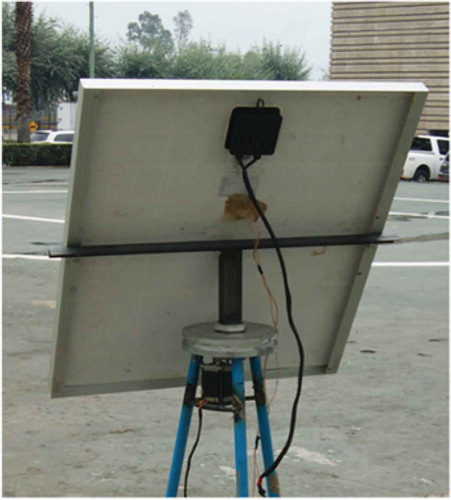
The proposed mechanical structure is based on two metallic discs, mounted over a tripod, which rotate around the azimuth axis. Over these discs a metallic arm holds a single solar panel that tilts on a vertical axis. Figure 1 presents the main mechanical structure used in the sun tracker system (Sinuhé et al. 2009). Sun trackers have been developed by different optimization structures and needs (Gomert 2010; Green 2014; Panait and Tudorache 2008; Liu et al. 2012).

Figure 1. Solar tracker structure.

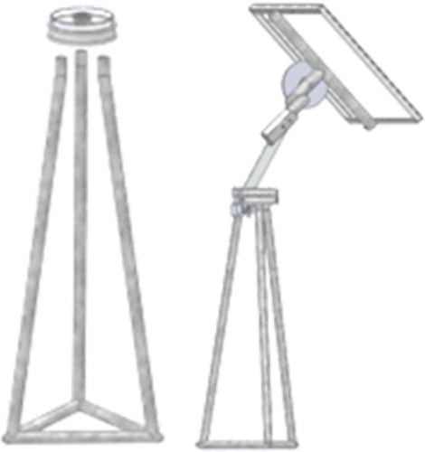
An alternative mechanical model is to set an arm over the head of the axis. The friction between the head of the axis and the disc could be minimized by placing a mechanical bearing. This structure moves by steeper motors and it is presented in Figure 2.

Figure 2. Alternative mechanical structure.

Position of the sun conventional method

Earth rotates around the sun in the vertical axis of the sun. It is well known that Earth declines at an angle of 23.45° from the axis parallel to the vertical axis of the sun. The axis from the sun to Earth and the vertical axis of Earth form an angle called solar declination. In other words, this declination is the same value as the latitude at which the sun is directly overhead at solar noon on each day. The solar declination angle is derived as

(1)

where is the number of the day starting at January 1 equals 1. The angle between a line collinear with the sun’s ray and the horizontal plane (perpendicular to the vertical axis) is called solar altitude angle. Thus, the solar zenith angle is the angle between the sun’s ray and the vertical axis:

(2)

In contrast, the latter two angles are not related to the fundamental angles, known as hour angle, latitude, and declination. The hour angle is defined as the angle based on the nominal time of 24 hours that the sun moves 360° around the earth. This angle can be calculated by:

(3)

in which means the minutes from local solar noon. So, before noon, the minutes are negative and after noon they are positive. Finally, the latitude is the angle between the line from the center of the earth to the site and the equatorial plane.

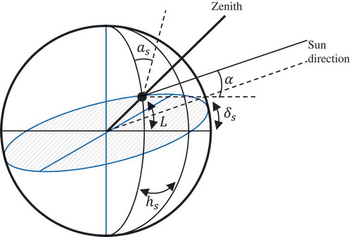
In order to know the position of the sun with respect to the center of Earth, two angles are needed: the solar altitude angle and the solar azimuth angle. The latter is the angle between the projection of the sun’s ray into the equatorial surface and the north–south line. These angles can be calculated as

(4)

(5)

Figure 3 summarizes those angles.

Figure 3. Geometric relationship between the sun and Earth.

Tracking angles

Chong and Wong (2008) derived a general formula for the tracking angles. They based its formula on mapping the incidence vector of the solar irradiation from the center of Earth to the surface, and then from the surface to the photovoltaic cell surface. Consider the incidence vector of the solar irradiation as

(6)

Then, the transformation matrix from the center of Earth to Earth–surface is derived as

(7)

Consider the as the coordinate values of the incidence vector of solar irradiation directly through the photovoltaic cell surface. They can be written from the axial tracking angle and the rotational tracking angle :

(8)

where is the angle between the horizontal reference axis from the photovoltaic cell surface and the incidence vector of solar irradiation directly through the cell surface.

Finally, the transformation matrix mapping from Earth–surface to the photovoltaic cell surface is produced by the product of the following transformation matrices:

(9)

(10)

(11)

(12)

where is the transformation matrix from Earth–surface to the photovoltaic cell surface, and are three tilted angles relative to Earth–surface frame. Notice that the photovoltaic cell surface is taken into account because the cell does not always fit parallel to Earth–surface, and the tilt angles correct this error.

Assuming that the incidence vector of the solar irradiation has to be equal to the perpendicular vector to the photovoltaic cell surface, then, the following equation holds:

(13)

Solving for the tracking angles (), the equations for a tracking solar system is defined as:

(14)

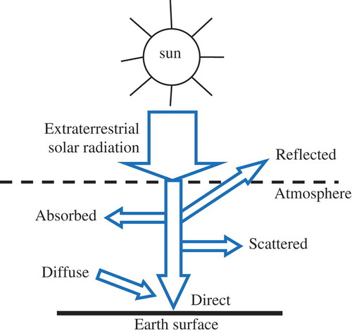
Thus, in order to obtain the maximum solar irradiation directly through the photovoltaic cell, Figure 4 shows the attenuation of the solar radiation passing through the atmosphere. Given the extraterrestrial solar radiation, a portion of this solar radiation is attenuated by absorption and scattering. The final incidence of solar radiation into Earth can be expressed as:

(15)

(16)

Figure 4. Solar radiation diagram.

where is the clearness number assuming as 1, being the optical depth that varies through months (see Table 1), is the day number counting from January 1st equal to 1, and is the constant value of radiation equal to 1353 W/m² (Goswami, Kreith, and Kreider 2000). Actually, the solar radiation received for the photovoltaic cell depends on the latter solar radiation, the incidence angle, and the tracking angle .

Table 1. Average values of optical depth and empirical sky diffuse factor measured every 21st day of month (adopted from Goswami, Kreith, and Kreider 2000).

Month	1	2	3	4	5	6	7	8	9	10	11	12
K	0.142	0.144	0.156	0.180	0.196	0.205	0.207	0.201	0.177	0.160	0.149	0.142
C	0.058	0.060	0.071	0.097	0.121	0.134	0.136	0.122	0.092	0.073	0.063	0.057

In order to determine the radiation, it is the sum of other radiations as the beam radiation, the sky diffuse, and the ground-reflected solar radiation. Each one is determined as follows:

(17)

(18)

(19)

(20)

(21)

where is the ground reflectance (approximately 0.2 for ground or grass, and 0.8 for snow (Goswami, Kreith, and Kreider 2000), and is the empirical sky diffuse factor that varies through the months.

Genetic algorithms adjusted for offline sun tracker

The tracking solar system is optimized for obtaining the best configuration points to which the photovoltaic cell has to be oriented in order to receive the maximum solar irradiation. In this sense, a configuration point is the ordered pair of tracking angles in which the photovoltaic cell is oriented (taking into account Equations (1) to (21)). Thus, a set of configuration points are expected for maximizing the solar irradiation. Genetic algorithms could be used for finding these configuration points.

Genetic algorithms are developed for this purpose. For instance, an individual is defined by 1440 genes in which each gene represents if the tracking solar system is moving in a minute of the day. If the moving value is 1, elsewhere is 0. An initial population is derived, then the fitness function is evaluated for each individual and all individuals are ordered from the best to the worst option for selection. After that, crossover and mutation are performed using probabilities, and a new population is derived.

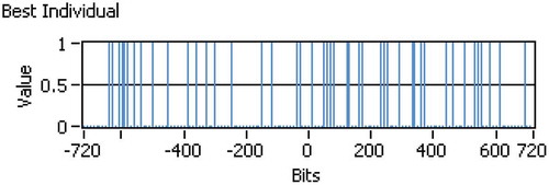
Using genetic algorithms, the tracking solar system was optimized. In this way, it was expected that genetic algorithms find the optimal position configurations in which the photovoltaic cell collects the most solar radiation possible, wasting the minimum power of actuators, and doing it in a minimum number of steps. For this purpose, an individual for genetic algorithms was designed as in which each bit represents whether the photovoltaic cell moves to the ideal best position (predicted by a conventional model of the sun tracker and the general formula for tracking angles) with the value TRUE or if the photovoltaic cell stands by in the previous position (FALSE). Notice that each bit represents the system configuration each minute, the reason why there are 144 bits for the 144 minutes over a day. Thus, the best solution expected is the set of position configurations during a day with minimum resolution of ten minutes.

Additionally, the fitness function was developed in order to reach the goal of this optimization: maximizing the collecting solar radiation and minimizing the power used by actuators.

The fitness function was created with the quadratic error average. For maximizing the power energy collected, a maximum upper limit (36 W are the maximum power supply by the photovoltaic cell) was selected as 40 W. Then, the power collected at the given time is compared with this upper limit. The error is then powered by two, and the sum of these quadratic errors is divided by the maximum number of time values (i.e., 144 in this case). As noticed, the maximum power collected per day is 3364 W. Thus, in terms of optimization, the error has to be decreased, and a better evaluation is needed. In this sense, the difference between the maximum power per day and the quadratic error is used. Finally, normalization is required. Second, for minimizing the power used for driving motors, it is required that the sum of the quadratic error has to be minimized. Following the previous process, the normalized evaluation is found for the number of times that motors are switched on. In mathematical terms, the fitness function is written as

(22)

In this way, the genetic algorithm was proved three times. For each running, the algorithm found three different solutions. Thus, looking at the results in Figure 5, the best solution was determined by the minimum function value. Five individuals were the population size with 0.95 of crossover probability, and 0.01 of mutation probability. Table 2 summarizes the set of tracking angle configurations and the time values for each configuration. Implementation of this optimization is presented in Figure 5. Because the genetic algorithm is proposed as an offline algorithm, the system is implemented in a personal computer running a LabVIEW program that has low calculation computer consumption, because the results of genetic algorithm optimization are included in a lookup table.

Table 2. Results of the genetic algorithm for optimizing the tracking solar system.

Sample	Best Fitness Function Value	Power Energy Collected	Number of Position Configurations
1	1.2931 @ 4,000 epochs	1314.80 W	45
2	1.2852 @ 4,000 epochs	1297.96 W	46
3	1.2721 @ 4,000 epochs	1292.05 W	46
Time [min]	Theta [°]	Beta [°]	Time [min]	Theta [°]	Beta [°]	Time [min]	Theta [°]	Beta [°]
00:00:00	90	0	07:50:00	73	120	16:10:00	73	240
01:20:00	161	99	09:30:00	54	136	16:50:00	81	244
01:30:00	159	99	10:00:00	50	142	17:30:00	90	248
01:50:00	154	99	11:20:00	41	166	17:40:00	92	249
02:00:00	152	99	11:30:00	41	169	18:00:00	97	250
02:10:00	149	99	12:50:00	42	198	18:10:00	99	251
02:20:00	147	100	13:00:00	43	201	19:20:00	115	255
02:40:00	142	100	13:10:00	44	204	19:40:00	119	256
03:00:00	138	101	13:20:00	45	207	20:20:00	129	258
03:40:00	129	102	14:00:00	50	218	20:50:00	135	259
04:30:00	117	104	14:10:00	51	220	21:00:00	138	259
05:30:00	103	108	14:40:00	56	226	21:10:00	140	260
06:00:00	97	110	14:50:00	58	228	21:40:00	147	260
06:30:00	90	112	15:50:00	69	237	22:10:00	154	261
07:00:00	84	115	16:00:00	71	239	23:30:00	173	253

Figure 5. Results of the angles to the tracking solar system.

As seen in Figure 6, the optimal tracking angles derived the response of power collected (black line). The total power collected per day was 1603.04 W. Contrasting this data with two responses for suboptimal tracking angles (red and blue lines), these angles collected 1673.13 W and 1591.95 W of power, respectively. These suboptimal tracking angles were modifications of the axial angle, five degrees less (red line response) and five degrees greater (blue line response) than the optimal axial angle found by genetic algorithms.

Figure 6. Response of the tracking solar system optimization.

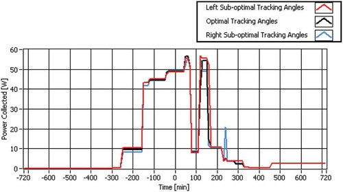
Analyzing optimal tracking angles, they derived a response slightly less significant than one of the responses of suboptimal tracking angles (red line). This happened because from 13:20 to 16:10 hours (or from minute 80 to minute 250) it became a cloudy afternoon. In fact, genetic algorithms found the best tracking angles for ideal conditions as a sunny day, not for cloudy or any other environmental condition (e.g., genetic algorithms considered 25°C of temperature). However, as noticed, the response in other time intervals was very close in all of these optimal and suboptimal positions.

Thus, it can be considered that genetic algorithms found well-tracking angles for positioning the photovoltaic cell. In addition, knowing that between the optimal and the left suboptimal (red line) responses was a relative similarity of 4.37%, and from the optimal to the right suboptimal (blue line) responses was a relative similarity of 0.69%; then, optimal tracking angles might respond to other environmental conditions, as clouds.

Finally, on the intervals from 00:10 to 07:50 hours (minute 710to minute 250) and from 17:30 to 23:50 hours (minute 330 to minute 710), the power collected is very small (less than 2.4 W/min). Thus, in these time intervals, tracking angles were taken off. Table 3 summarizes the 17 final optimal tracking angle positions.

Table 3. Seventeen final optimal tracking angle positions.

Time	Theta	Beta	Time	Theta	Beta
[min]	[°]	[°]	[min]	[°]	[°]
00:00:00	90	0	14:00:00	50	218
09:30:00	54	136	14:10:00	51	220
10:00:00	50	142	14:40:00	56	226
11:20:00	41	166	14:50:00	58	228
11:30:00	41	169	15:50:00	69	237
12:50:00	42	198	16:00:00	71	239
13:00:00	43	201	16:10:00	73	240
13:10:00	44	204	16:50:00	81	244
13:20:00	45	207

Design of intelligent water drop algorithm for sun tracker

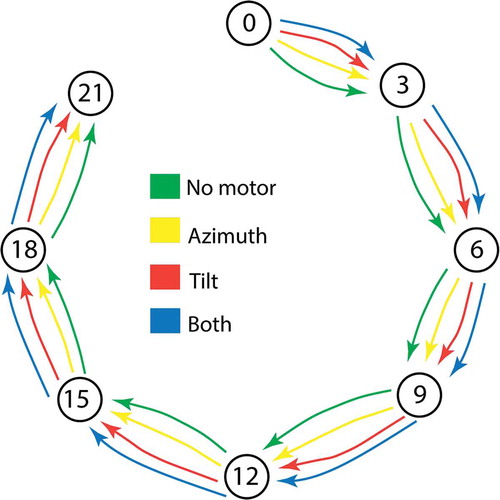
The basic structure of the algorithm is presented in Figure 7, where the IWD algorithm is presented for sun tracker optimization. Each circle represents a time of the day. For this case, the day was divided into 15-minute lapses, giving a total of 96 nodes. As can be seen, a directed graph was created where each node can move only to the next one by choosing one of four paths. The four paths represent the four combinations of moving and not moving the two motors to align the module to the average expected sun rays in the 15-minute lapse.

Figure 7. Description of the IWD algorithm.

This structure was derived from the application to image segmentation mentioned by dos Santos (2009). The basic strategy is to let the water drops try to choose the best way. Because the heuristic for the IWD algorithm was chosen to be the expected energy gain, the algorithm should converge to the optimum solution naturally.

A computational test was done on March 12 in Mexico City. The temperature was simulated using a basic Gaussian function, as shown in Equation (23).

(23)

where t- is the time of the day given in minutes.

This function will give the temperature in a range between 5°C and 25°C, with its highest point at 12:00 p.m. and a width given by 360²; Figure 8 describes the temperature function.

Figure 8. Plot of the temperature function.

The stepper motors were simulated by constants in Wh /(degree moved). So the total energy subtracted from the energy received from the PV-module is derived from Equation (24)

(24)

where

P_tot is the total power to be received

P_PV is the raw power given by the PV-module

C_M is the motor constant in [Wh/degree] and could be accounting for the change in angle and the rotational speed of the motor.

It is evident that the motors have an average power consumption of times the motor constant. Of course, this equation reduces to just the first operand of the right side once the motor reaches its objective angle and stops moving. In this case, both motors have the same parameters, but their gear relationships are different. The azimuth motor has a gear system that decreases the rotational speed by 98.068%. The tilt motor has a gear system that decreases the rotational speed by 95.774%

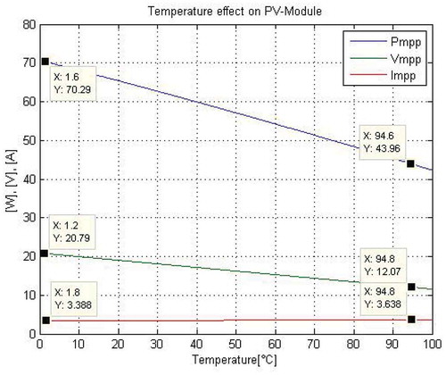
Both motors are rated nominally at 12 V 4A and 1.8° per step. The real values differed from the nominal operating point, namely 12 V 1.33A for both motors. Because of the gear system, the 1.8° per step went down to 0.034° for the azimuth motor and 0.075° for the tilt motor. The power delivered by the PV-module was simulated to be always in the MPP affected by the temperature. The Equation (25) is applied.

(25)

where

P_PVT is the power as a function of temperature in °C.

I_mpp is the cell MPP current given value

Vmpp is the cell MPP voltage given value, C_Impp and C_Vmpp are the cell temperature coefficients given in [A/°C] and [V/°C], respectively, and T is the temperature. The temperature effect is presented in Figure 9.

Figure 9. Temperature effect on the PV-Module.

Aside from these equations, power losses due to air mass (AM) and misalignment were taken into account using the Equations (26) and (27).

(26)

(27)

The complete system was simulated as a C program in the GCC compiler (Stallman 2012). Figure 10 displays paths of soil across the day.

Figure 10. Paths of soil across the day.

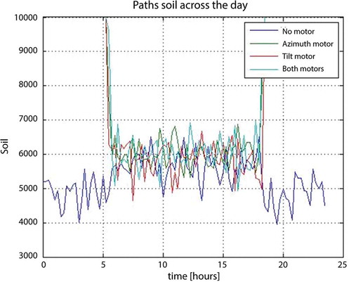
The best form for using this information is like probabilities. So the probability of not moving a motor is 1− soil. The information is not normalized. As expected, the motors will be active only when the sun comes out. The information seems to be really noisy. This is to be expected because the algorithm is based on probability and random variables. Finally, the raw electric power for an MPP-Tracker system is shown in Figure 11.

Figure 11. Algorithm output.

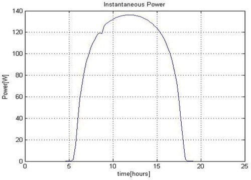
It can be seen how the IWD algorithm maximizes the power gained. The small asymmetry by the 8th hour is the result of the algorithm converging to the wrong paths. Given its probabilistic nature, this can be sometimes expected, but should be avoided by using more drops.

The curve is still very ideal. Irradiance noise (clouds, solar fluctuation, pollution, etc.) was not included in the simulation.

Sun angle description for water drops

The IWD algorithm needs to know the incoming irradiance vector angles. In order to get the desired vector, two auxiliary angles have to be calculated: the declination angle and the hourly angle. For the declination angle (δ) Equation (28) is used:

(28)

For the hourly angle (ω), the Equation number (29) was used:

(29)

Then, by using these angles, we could proceed to calculate the final azimuth (A) and altitude (α) angles with Equation (30).

(30)

For calculation of the azimuth, the next equations are needed. The conditions are presented following.

If

(31)

then

(32)

else

(33)

where

(34)

It is necessary to add the AM in order to be able to predict the solar irradiance on the cell, which is done by 13 (taken from Meinel and Meinel 1976 and from Schoenberg 1929):

(35)

For the implementation, an algorithm was derived starting with the structure proposed by (dos Santos 2009). The equations below are included in the pseudocode as the main part of the optimization process.

(36)

(37)

(38)

(39)

(40)

(41)

Intelligent water drops for online sun tracker

The conditions for generating an algorithm that optimizes the sun tracker moment are limited according to the mechanical and electronic system, this optimization proposed tries to limit the number of sensors and additional components in order to calculate the next sun tracker position. Corio, Reed, and Fraas (2010) present diverse options for sun trackers and shows the benefits of using the sun tracker. The steps below are proposed for using the IWD as the core inside the sun tracker:

1. Variable definition: Specifically av, bv, cv, as, bs, csα, θ, ρ_n initialize soils as InitSoil, cell-temperature coefficients and motor-energy coefficients.

   1. Iterate over the times the algorithm is going to run.

   2. Recalculate soils as . This is done in order that, through iterations, the past solutions affect the soil already eroded.

   3. Reinitialize drops with default values.

   4. Iterate over the nodes (it can be seen as iterating over the whole day going at 15-minute intervals).

   5. Calculate the sun position and the AM for the 15 minutes in the current lapse.

   6. Calculate the sun’s average position for the next 15 minutes.

   7. Iterate over each intelligent drop.

   8. Calculate the probability distribution for each of the movements (probability depends on the soil amount of each of the four paths).

   9. Calculate a random number.

   10. Go to the code portion of the path “chosen” by the random number. So, if the probabilities are 20, 20, 25, and 35 for no motor, azimuth motor, tilt motor, and both, respectively, and the random number is 60, then it will go to the tilt section because the random number is between 40 and 65.

   11. If the path implies moving a motor, because each drop has its own module representation, calculate the degrees to move the module and update the module’s angle to the sun’s incoming rays at the average time of the 15-minute lapse.

   12. Calculate the velocity of the current drop as in Equation (14), where soil is the soil of the path chosen.

   13. Calculate the Eu as in Equation (15); P_M is the motor average power, T_M is the time the motor takes to travel one step (1.8°). PI/100 is to translate into degrees, and 3600 is to go from Joules to Wh.

   14. Calculate Eg as in Equation (16) where P_PV is the average power during the minute lapse. The 60 gives us the corresponding 1-minute lapse.

   15. Calculate the heuristic HUD as in Equation (17).

   16. Calculate the change in soil as in Equation (18) with the velocity and HUD already calculated.

(2) Update the current path’s soil.

Once the path’s final soil has been calculated, traverse the graph, choosing always the lowest soil, and on each node, fill the move_table array with the corresponding number. For instance, if the next smallest path is the tilt-motor path, then in the move_table array at the next node’s index, write a 2 (no motor is 0, azimuth is 1, and both is 3).

Return the move_table so that it is used throughout the day. When it is used, a conventional sun tracker optimization is based on external information; the system requires information from different equipment such as the GPS, the pyrometer, and the anemometer. Those elements are needed inside the optimization topology and the total cost increase; this is the case of the optimization proposed by Engin and Engin (2013). The basic flow diagram for optimization based on external information is presented in Figure 12.

Figure 12. Flow diagram of optimization based on external information (Engin and Engin 2013).

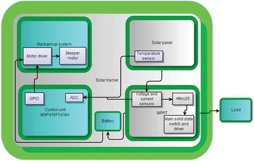
The system proposed uses temperature, voltage, and current sensor, but those sensors are also used for the maximum power point tracking (MPPT) that is a technique for getting the maximum possible power from one or more photovoltaic devices (Hua and Shen 1998). Solar cells have a complex relationship among solar irradiation, temperature, and total resistance that produces a nonlinear output efficiency, which can be determined using the I-V curve; thus, the purpose of the MPPT system is to sample the output of the cells and apply the proper load to get the maximum power for any given environmental conditions. As can be seen, the sensors do not add additional elements. The methodology proposed used the sensor needed in the MPPT for obtaining the sun tracker optimization. A complete diagram of the proposed system is presented in Figure 13. For implementing the sun tracker optimization, several conditions have to be taken into account, thus, the energy efficiency of its components is very important. The MSP-EXP430F5438 board was selected as the microcontroller that runs the optimization system because it has the inputs and outputs conditions as well as low energy consumption.

Figure 13. Complete diagram of the proposed sun tracker.

Experimental results of IWD algorithm

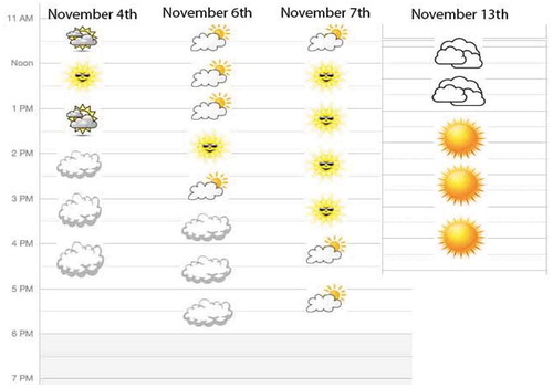
A set of tests was done in order to validate the proposed algorithm. The first tests were carried out in November 2012 in Mexico City under the battery-charging condition; Figure 14 shows the weather conditions.

Figure 14. Test’s weather calendar.

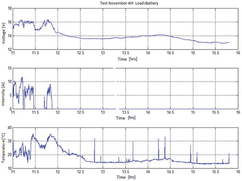
The data recorded was taken by three sensors (voltage, current, and temperature). The MPPT board provided the voltage and current sensors. The temperature sensor was fed directly to the ADC of the microcontroller. Each sensor was sampled every 10 seconds. For the solar panel, a 60-W solar module mounted on the moving mechanism was used, which changed the azimuth angle. The tilt angle was stable at 43°. For the algorithm, the IWD table was used. As load, we used a 12-V 20Ah half-charged battery, which also provided the energy that the motor used to move the solar panel.

Five conclusive tests were carried out and these are presented in Table 4.

Table 4. Experiments for evaluating the IWD.

Number	Date	Name
1	5/11/2012	Moving panel with IWD algorithm charging a battery
2	6/11/2012	Moving panel with IWD algorithm feeding a 10kΩ resistance
3	7/11/2012	Comparison between a static panel and a constant movement panel
4	13/11/2012	Comparison between a static panel and a IWD moving panel with 3Ω load
5	13/11/2012	Motor energy consumption

In Figure 15, there are three variables plotted (voltage of the solar panel, current of the solar panel, and temperature of the panel, accordingly). The panel received plenty of energy from the sun during the interval from 11 a.m. to 12 a.m.. This is supported by the voltage and temperature graphs.

Figure 15. Test results graph for battery as load, November 4th.

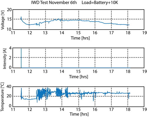
The second test was run on November 6, 2012 in Mexico City. Each sensor was sampled every 10 seconds. For the solar panel, a 60-W solar module mounted on the moving mechanism was used, which changed the azimuth angle. The tilt angle was stable at 43°. For the algorithm the IWD table of movements was used. As load, a 10kΩ resistor was used. A 12-V battery provided power to the electronic circuits and the motor used to move the mechanism. The main objective of this test was to evaluate the behavior of the system with a constant load rather than a battery. The data recorded by the sensors is presented in Figure 16.

Figure 16. Test result graph with a large resistor as load.

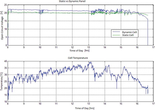
The third test was run on November 7, 2012 in Mexico City. For the static panel a 60-W solar module was used. The angles for this second panel were taken as optimal when the sun was at its highest point in the sky: 43° for the tilt angle and 90° taken from the east for the azimuth angle. Both panels were left unconnected in order to measure the open circuit voltage (Voc). A 12-V battery was used to power the electronic circuits and the motor used to move the mechanism. The main objective here was to compare the Voc of the two panels.

Two graphs are shown in Figure 17. The first plot contains the voltage data for the two panels during the measurement time. The second graph depicts the measured temperature during the day. The first fact that stands out is the temperature readings. When compared to the previous tests, one can safely deduce that the whole day was clear. And indeed it was. Aside from some scarce clouds, most of the energy was received through direct radiation from the sun. Now, turning to the voltage graph, it can be seen how both panels follow the same pattern with a difference of a voltage offset of roughly two volts. The noise shown after 13 hours is due to some shadows that partially blocked the panels.

Figure 17. Test result graph comparing static and dynamic cell, November 7th.

The fourth test was run on November 13, 2012 in Mexico City. Both panels were connected to a 3Ω resistor. For each panel, four wire-wound ceramic 25-W resistors connected in parallel were used. Two of them were rated at 15Ω and the other two were rated at 10Ω. Figure 18 presents the data recorded.

Figure 18. Test result graph using low resistance as load, November 13th.

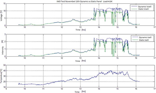
Starting off the analysis with voltage and current (which are almost the same) graphs, we can infer the climate that ensued during the test. For the first half of the day, it was very cloudy and only diffuse radiation was received. Because of the low resistance, the diffuse radiation could not give enough energy for the panels to maintain a high voltage. However, as the time reached 13:40 a strong change can be seen. This is due to the fact that the clouds are grouped in relative tight packs, leaving the radiation signal almost discrete: cloud or no cloud. For the rest of the day, the sky was almost always clear. Important facts to notice with regard to these two graphs are that the voltage and current are almost equal at 12:00 p.m. This is in accordance with the panel’s respective alignments. As the moving panel follows the sun, at noon, its azimuth angle is the same as that of the stationary one. This, then, gives the same irradiation for both panels, which reflects on having almost the same voltage and current. After 12 p.m., it can be seen how the boundary between both lines broadens as the sun moves away from its noon location in the sky. Another very important fact that stands out specifically in this test is the fact that the temperature, the voltage, and hence, probably also the radiation, follow the same pattern. In contrast to the other test, this is accomplished by having sufficiently low enough resistance values in order to operate in the more linear zone of the power plot of the solar panel in regard to the voltage and current fluctuations.

However, it is important to know the total energy consumed in a day by moving the panel every half hour, and by moving the panel through the day using the IWD algorithm. First measured was the consumption of the motor in a constant moving panel. These were the results: For the constant moving panel, it was reported that only 950 J were used throughout the day. For the IWD panel, it was found that 630 J were used.

These observations are congruent to the fact that the more times you have to move the panel throughout the day, the more energy will be consumed. This is because almost all the energy goes into breaking the static friction together with the panel’s rotational inertia. This is why the constant moving panel (which moved more times in a day than the IWD algorithm) consumed more energy.

Discussion

Because sun tracker systems are designed for getting more solar energy than static solar cells, it is very important to focus on algorithms for finding the optimal position of the sun tracker. For offline algorithms, it is recommended to apply genetic algorithms for usage in distinct geographical regions where the meteorological conditions are almost constant, deriving the configurations at which photovoltaic cells have to be located for maximizing the collecting solar radiation, and minimizing the usage of power energy for driving the sun tracker. This method could be implemented in a low-cost microprocessor using a lookup table for locating the tracking solar system.

However, in places where meteorological conditions are changing drastically over weeks, it is a better option to apply swarm optimization, which is a faster algorithm. The fastest response of the water drops algorithm allows using it under big weather disturbances during a day. The algorithm has to be implemented in a more powerful microprocessor than does the genetic algorithm, which is an offline method.

Both the genetics algorithm and the water drops have to be adjusted for solving the sun tracker trajectory; also, the digital platform has to be modified in order to have a correct implementation.

Conclusions

The proposed algorithm for tracking the sun and getting a maximum electrical energy works well under different environmental conditions. The sensors included are also used in the maximum tracking point, so the cost of the whole system is inexpensive. The computational cost is lower when genetic algorithms are used and the computational cost increases when water drops are implemented. The genetic algorithms present good results when the weather conditions are almost constant or low disturbances are presented.

When a partially clouded day appears, the system can increase the energy by 40% by using the IWD tracking mechanism. If the day is clear, the energy increments around 50%. On a cloudy day, it makes no sense to use the optimization algorithm because the sun tracker does not increase the energy. That means that for geographical regions where there are mostly cloudy days, this technology is not to be recommended and a static solar cell is recommended. The energy taken by the motor to rotate the solar panel is negligible. Therefore, by adding a tilt motor to adjust this angle, the percentage of energy gained could go up. The design and implementation show the possibility of using the IWD in a big solar cell array collocated in a sun tracker system. The microcontroller selected for running the algorithm is ideal for this application because the whole algorithm is compact and the real-time implementation is possible under time conditions.

References

- Chong, K., and C. Wong. 2008. General formula for on-axis sun-tracking system and its application in improving tracking accuracy of solar collector. Solar Energy 83 (3):298–305.
- Corio, R., M. Reed, and L. Fraas. 2010. Tracking the sun for more kilowatt hour and lower-cost solar electricity. In Solar cells and their applications, 207–217. New York, NY: John Wiley & Sons.
- Dariane, A. B., and S. Sarani. 2013. Application of intelligent water drops algorithm. Dordrecht: Springer Science+Business Media.
- dos Santos, W. P. 2009. Evolutionary computation. ISBN 978-953-307-008-7.
- Engin, M., and D. Engin. 2013. Optimization controller for mechatronic sun tracking system to improve performance. Advances in Mechanical Engineering 2013 ( Article ID 146352): 9 pp.
- Gomert, A. 2010. Concentrator photovoltaics: a mature technology for solar power plants. Retrieved from http://www.renewableenergyworld.com/articles/print/pvw/volume-2/issue-3/solar-energy/concentrator-photovoltaics-a-mature-technology-for-solar-power-plants.html
- Goswami, D. Y., F. Kreith, and J. F. Kreider. 2000. Principles of solar engineering. CRC Press.
- Green, M. A. 2014. Clean electricity from photovoltaics. In Series on photoconversion of solar energy, Vol. 1, ed. M. D. Archer and R. Hill. London, UK: Imperial College Press.
- Hua, C., and C. Shen. 1998. Comparative study of peak power tracking techniques for solar storage system. Applied Power Electronics Conference and Exposition 2:679–685.
- Liu, Q., M. Yang, J. Lei, H. Jin, Z. Gao, and Y. Wang. 2012. Modeling and optimizing parabolic trough solar collector systems using the least squares support vector machine method. Solar Energy 86 (7):1973–1980. doi:10.1016/j.solener.2012.01.026.
- MacDonald, W. S. 2011. Solar access measurement device, Patent No. 7873490. Washington, DC: U.S. Patent and Trademark Office.
- Meinel, A. B., and M. P. Meinel. 1976. Applied solar energy. Boston, MA: Addison Wesley.
- Mitchell, M. 1999. An introduction to genetic algorithms. A Bradford Book. Cambridge, MA: The MIT Press.
- Panait, M. A., and T. Tudorache. 2008. A simple neural network solar tracker for optimizing conversion efficiency in off-grid solar generator. Paper presented at the International Conference on Renewable Energy and Power Quality, March, 2008, Santander, Spain.
- Raihanul Islam, M., and M. Sohel Rahman. 2013. An improved intelligent water drop algorithm for a real-life waste collection problem. In Advances in swarm intelligence, Lecture Notes in Computer Science Volume 7929, 472–479.
- Schoenberg, E. 1929. Theoretische Photometrie, Über die Extinktion des Lichtes in der Erdatmosphäre. In Handbuch der Astrophysik. Band II, erste Hälfte (pp. 1–280). Berlin, Germany: Springer.
- Sinuhé, F. M. Jiménez, S. De Jesús Castro Molina and R. Vargas Sandoval. 2009. “Alternative energy, wind and solar.” Master’s diss, Tecnologico de Monterrey campus ciudad de Mexico.
- Stallman, R. M. 2012. GNU compiler collection internals. Free Software Foundation. Retrieved from http://gcc.gnu.org/