
ABSTRACT
Energy-supply issues constitute one of the most important issues that we face nowadays. Before a viable alternative energy source of supply is discovered and implemented, saving energy is essential. To improve the energy economizing of actuators, this work proposes a method based on fuzzy logic for scheduling and controlling electrical operators in a cyber-physical system. With the feedbacks of sensor data including output of process and the environmental variations, the intelligent controller can gather the current situation and predicted trend. After analyzing the data with the fuzzy rule, the actuators are controlled with the consideration of the desired set point and energy economizing. The results of a simulation reveal that the fuzzy control method for actuators in a cyber-physical system can be used to minimize the power consumption of the system while accomplishing the desired set point.
Introduction
The various significant problems stemming from energy production and consumption have been attracting considerable attention in the past several decades, and the sense of urgency regarding the need for solutions is perhaps greater than ever. Energy-supply issues have become more pressing than ever. In the absence of any viable alternative energy supply, perhaps the best approach to addressing this and other energy-related issues should center on reductions in energy consumption. Researchers have been working on cyber-physical systems involving different techniques, but most having the same goal: an adequate control of processes resulting in the achievement of desired values. The power consumption of systems is rarely considered. This work aims at both achieving the desired reference values and minimizing the power consumption of the given system.
Various cyber-physical systems (Wolf Citation2009) are utilized in everyday life. They play important roles in such diverse areas as automotives, process control, manufacturing, chemical processing, networked building control, transportation, smart-home networking, health care, and other fields. Human lives benefit greatly from cyber-physical systems. With time, the power consumption of cyber-physical systems is increasing with their scale. As a population, we have a pressing obligation to consider how we can reduce our consumption of power while satisfying reasonable demand, and the current study’s proposed approach is a worthy step in this direction.
Many mathematicians and scientists have developed the concept of control theory. In the 19th century, Hall conceptualized the need for fluctuations in control theory (Hall Citation1907). Bellman’s invention of dynamic programming and Pontryagin’s contribution to the concept of maximum principle also helped to establish the foundations of modern control theory (Andrei Citation2005). Wiener introduced the concepts of positive and negative feedback (Rosenblueth, Wiener, and Bigelow Citation1943), which have since been applied in many fields of research including engineering, control systems (Stankovic et al. Citation1999), cyber physical systems (Liu et al. Citation2011), and computer science.
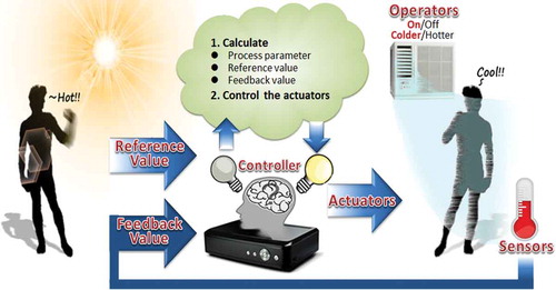
Most feedback cyber-physical systems are composed of a central computational controller for controlling the actuators, actuators for controlling the operational physical devices, operational physical devices for affecting the physical quantity, and sensors for monitoring (see ).The set point, or reference value, is a desired value of a physical quantity. When the system is operational, the current output, called the process variable, is monitored. In the central computational controller, the controller calculates the difference between the process parameter and the set point and uses this difference as a feedback value to compensate for error in the previous state.
Figure 1. Scheme of a cyber-physical system.
In contrast with a feedback system, an open-loop system does not have any sensors to monitor the results of the system. It does not guarantee the performance of the system unless the relationship between inputs and outputs is well modeled mathematically.
In this work, a feedback cyber-physical system is implemented as a method for controlling actuators in the system. The inherent feedback aspect of the system takes into account not only the gap between the set point and the process variable but also environmental variations. The system collection of sensor data and prediction of environment variation trends would rest on the well-known “weighted least square error” algorithm. We expect that this method could minimize the power consumption of the system’s electrical operators while achieving the desired set point.
In our system, a set of physical operators of the same function, which affect the same physical quantity, are considered. Each physical operator might have a different capability to affect the target and consume a different level of energy. The physical operators should provide the capability level and the power-consumption level of each physical device. One set of sensors is placed dispersedly around the affected area for process-variable monitoring. Another set of sensors collects the environmental variation. The sensors push the readings in digital form periodically to the central controller.
The proposed controller of the system herein has two main parts. One is a central control module; the other is set of actuator controllers, which implement fuzzy control according to the proposed fuzzy rules. The central control module plays a managing role in the system. The module delivers information about each operator to the corresponding actuator controller. The remainder of this article is organized as follows: “Related Work”
reviews some related works. “System Model and Fuzzy Rules” presents both the system model to which we apply our method and the details of our proposed “fuzzy-based actuator control” method, which should minimize the power consumption of the electrical operators without obstructing the achievement of the desired sensor value. “Simulation” presents the performance analysis. Finally, in ”Conclusions,” we lay out some important conclusions drawn from the findings.
Related work
A variety of approaches for controlling actuators in a cyber-physical system have been proposed (Ilić et al. Citation2010; Poovendran Citation2010). Branch, Chen, and Szymanski (Citation2008) proposed an auction-based method as a basis for distributed actuator coordination within their Sentire sensor and actuator networks. That study’s primary goal was to coordinate actuators that were distributed in several places in a way that would facilitate the even allocation of energy resources. However, the desired temperature could not be achieved in several locations simultaneously. Xia, Sun, and Tian (Citation2009) proposed a GA-based, two-stage fuzzy temperature-control algorithm for industrial furnaces. According to their simulation results, the combination could reduce the number of fuzzy rules and keep the temperature around the set point, but only under the condition that the characteristic of thermal conductivity could be grasped. Furthermore, the cited study addresses neither fuel consumption nor fuel-efficiency performance.
We believe that the motivation of intentions is to improve people’s lives through their use of a product or service, and people who use the product or service want to extract some benefit from it. Therefore, the goal of this work, as described above, is to minimize a given system’s power consumption without obstructing the system operations’ achievement of the desired sensor value. Fuzzy control is a well-known and popular method for solving control problems. Many studies have found it to be effective. This study will provide fuzzy rules for fuzzy control in order to reduce the power consumption of this system while still realizing the desired reference value. The fuzzy control method is briefly introduced following.
Fuzzy logic has been applied in many control systems. Feng, Gong, and Yang (Citation2009) utilized a fuzzy logic control algorithm to control the temperature of oil in a large hydraulic system. Li, Chang, and Tong (Citation2004) successfully designed a real-time fuzzy target-tracking control scheme for autonomous mobile robots, based on fuzzy logic. The general process of fuzzy control is as follows.
Fuzzification: Fuzzification is the conversion of numerical inputs into fuzzy linguistic terms using membership functions.
Creating fuzzy rules: Fuzzy rules are the core of fuzzy logic. They are usually based on human experience and expert knowledge.
Fuzzy Logic Inference: Fuzzy logic inference is a method by which a fuzzy control query table that is constructed according to the fuzzy rules provides an output fuzzy set.
Defuzzification: In defuzzification, the output fuzzy set is transformed into a single number as the output of the fuzzy control.
One of the advantages of fuzzy control is that its implementation is relatively fast. Fuzzy rules have a key role in the control. The generating fuzzy rules depend greatly on experience and an understanding of the system. This work will provide some rules for solving problems of power consumption of a system while the desired value is still achieved.
Genetic algorithm (GA) is a widely applied concept in many control systems. Aytug and Koehler (Citation1996) analyzed the runtime complexity of a genetic algorithm. They found a new stopping criterion for genetic algorithms by which the number of iterations required to find an optimal solution with a desired level of confidence is bounded (1996).
Sharapov and Lapshin (Citation2006) conducted significant research on the convergence of GAs. Aytug and Koehler (Citation2000) and Sharapov and Lapshin (Citation2006) found that string length, mutation rate, and population size can affect the convergence time of a GA.
In this work, performances of the system are compared, first by harnessing a GA-based control method and then using the proposed fuzzy logic method.
System model and fuzzy rules
System model
This section presents and explains the proposed system model. As shown in , the system is based on a feedback cyber-physical system. The actuators in the system serve to control physical operators. The system includes two sets of sensors that monitor the same physical quantity. One set of sensors is evenly distributed to monitor the output values of the processes. These sensors monitor output values and periodically transfer them to the central control module. The other set of sensors are dispersed in a nearby environment to monitor variations. The environmental values of sensors are delivered continuously to the weighted least squares error (WLSE) predictor. WLSE is a well-known prediction algorithm, which is in the proposed system for environmental-variation prediction.
Figure 2. System model.
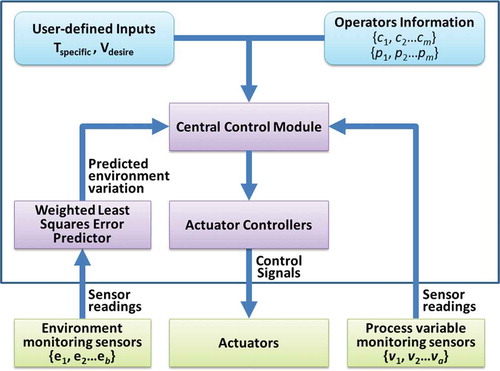
In the WLSE algorithm, from a set of inputs, a weighted sum of errors is calculated and minimized for a given set of weightings of those inputs. A new set of coefficients for the current time is then generated. These coefficients are used to predict the new value at the next instant. A detailed mathematical treatment of the WLSE can be found elsewhere (Monzingo and Miller Citation1980).
The predictor can store historical readings of the environmental sensors, and these old data are de-emphasized by applying the weights. The value that results from the WLSE predictor is delivered to the central control module.
The central control module manages the system. It copes with all variables, including the output of the process, and the predicted temperature variation in the next instant. The central control module delivers the same process variable and predicted environmental variation to all actuator controllers and corresponding information to each actuator controller, respectively.
The fuzzy control method is utilized in the system. Fuzzy controllers control the actuators according to the proposed fuzzy rules. The power consumption of the whole system is, thus, reduced while the desired reference sensor value is realized.
Information about each physical operator, including its capacity and power consumption, is assumed to be known. Before the system is operated, the user can determine the total operating time and the target value for the system. explains the symbols.
Table 1. Summary of notation.
Definitions of parameters
Before the fuzzy rules are demonstrated, some parameters are defined and assumptions explicated. Consider m operators and actuators in the system of interest. One actuator controls one operator. As described, the operators in the system have different capabilities, c1, c2…cm, and the power consumption, p1, p2…pm, of each operator is known. The operators additively affect the same process variable.
A user can determine operational time of the system, Tspecific, and the desired reference sensor value, Vdesired, to be achieved. The system starts to operate at time Tstart and stops operating when the system has been running for Tspecific.
Readings of sensors that are placed around the area to be affected, v1, v2… va, are transferred to the central control module. The mean value, Vread, of the sensor readings is calculated and feedback to the central control module. The initial sensor reading at Tstart is Vinitial.
Weighted least squares error
The readings, e1, e2…eb, of the environmental sensors are delivered to the predictor to predict the environmental variation in the next instant. The mean reading, Emean(k), of the environmental sensors is recorded at every instant. Then, the mean environmental variation per unit time, Vvar, is input to the WLSE algorithm.
where Emean is the mean environmental sensor reading at time k; Emean(k-1) is the mean environmental sensor reading at time t = k−1; M is the number of historical data considered.
In the WLSEalgorithm, the previous M historical values in vector form are multiplied by a vector of coefficients to produce a new predicted value,.
where u(k) is the vector of the M preceding values at time t = k,
and is a coefficient vector at time t = k−1. The coefficient vector can be determined as follows with aM(1) = [1,0,0…0]T and P(1) = I at the beginning of the algorithm.
In the above equations, M is the order of the predictor and α is the weight. The weights of older values are set to de-emphasize old values, αk = αk−1, where α < 1 and is usually set to 0.99.
Fuzzy control algorithm
To demonstrate accurately the fuzzy rule, a scenario that involves a temperature control system is considered. Assume that the goal of the operating the system is to maintain the room temperature around 26°C. Each heater and each cooler has one fuzzy control. The heater and cooler have the same membership functions but implement different fuzzy rules. As described, a WLSE predictor predicts the environmental variation in the next instant. The capabilities and power consumptions of the operators are provided and can be accessed by the central control module. This example can be easily generalized to other cyber-physical systems and, so, serves as a paradigm of fuzzy rules.
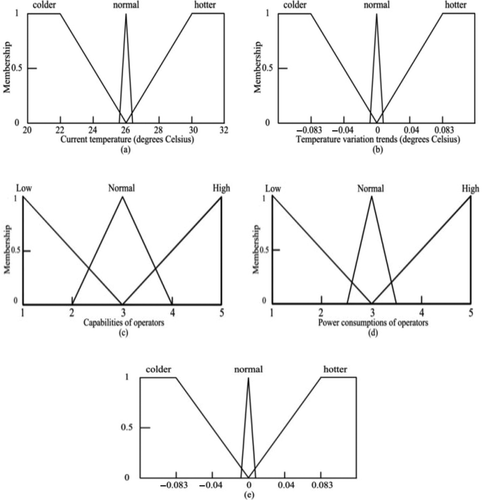
The fuzzy control has three inputs and one output. The inputs are current temperature, capability level, and power level. The membership functions for the inputs are designed here.
shows the membership functions for the input variables current temperature, capability, and power consumption. presents the membership function of the output variable. The horizontal axes in represents current temperature in degree Celsius, power consumption in Joules, per unit time (°C/min), and power consumption of operator per unit time (J/min), respectively.
Figure 3. The membership functions.
The fuzzy rules for temperature control build on some basic principles.
Normal state: If the current process variable is in the normal state, meaning the current temperature of the room after the operation of the heaters or coolers, the corresponding operator works only if its capability is high and its power consumption is low.
Positive state: If the process variable exceeds its normal value, meaning that the temperature is higher in the case of heating or cold in the case of cooling, no operator functions.
Negative state: If the process variable is less than its normal value, meaning that the temperature is low in the case of heating or hot in the case of cooling, the fuzzy rules are more complicated than under the previously listed two conditions. Basically, the operators are on if their capability is high and their power consumption is low.
and on the last page of this article presents details of the fuzzy rules that apply when coolers and heaters operate.
Table 2. Fuzzy rules for heaters.
Table 3. Fuzzy rules for coolers.
Simulation
Simulation parameters
The operation of the system was simulated in MATLAB. The performance of four methods is compared including the fuzzy logic control method implementing the fuzzy rules proposed herein, a GA-based method, the Simple-Top method and the Simple-Middle method. The GA-based method generates a schedule that is to be followed by operators in the system. Each gene in a chromosome represents the operating time of operators, such that a chromosome represents the operating times of all operators in the system. Simple-Top is a method that always selects the operator with the greatest capacity to operate in the system. Simple-Middle is a method that always chooses an operator with the capacity to operate.
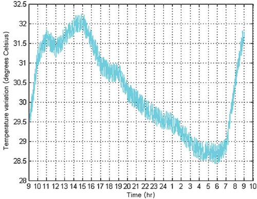
The physical operators in the system are assumed to be heaters and coolers. Let the numbers of both heaters and coolers be five. The heaters increase the temperature by {0.0167, 0.033, 0.05, 0.066, 0.083} degrees Celsius per minute, whereas the coolers reduce the temperature by {0.0167, 0.033, 0.05, 0.066, 0.083} degrees Celsius per minute in a room of size = 10 m x 10 m x 4 m. The power consumptions of both sets of heaters and coolers are {1, 2.5, 5, 6.5, 8} J per minute. Let the physical quantity to be affected be temperature. The average temperature variation, recorded by the Taiwan Central Weather Bureau between May and June 2011 in Tainan city, is used as the environmental variation.
In the simulations, the system operates for 24 hours from 9 a.m. The desired reference is set 26°C, and the initial sensor reading at the system start time is 29.3°C. The simulations are run 50 times and the following figures show the final average property. presents the values of the parameters.
Table 4. Parameters of the simulation.
GA control
In this simulation, there is one GA control for each heater and each cooler. “Period of time” is designed as the desired first hit time value, Thit. All available influential operators, when in operation, can first help achieve the system’s desired reference value. The first hit time may vary in accordance with the actual condition of the implementation system. The higher the system capability, the shorter the hit time is. The period of time as epoch time, Tepoch, in the system is integrated for GA control. At every start time of an epoch, the operators in the system will be rescheduled according to the current process variable and environmental-variation trend.
The binary-coded standard GA is adopted by researches (Aytug and Koehler Citation2000; Sharapov and Lapshin Citation2006) as a scheduler to schedule and control the operators. The structure is as follows:
Initialization: An initial population is generated with n individuals.
Evaluation: The objective value of each individual in the population is evaluated. Using linear ranking, we then determine the fitness value of these individuals according to the objective value. The implementations of an objective function are to evaluate the capabilities and power consumption of individuals during an epoch time, compute the capability gap, and evaluate a given objective value.
Repetition: Repeat three steps until the exit condition is satisfied. The first is to select parents from the population according to their fitness values. The second is to perform crossover and mutation in relation to the population to produce a new population. The final is to evaluate the fitness values of the new population.
Stop: If the exit condition is satisfied, stop and return to the best solution in the current population.
Performance evaluation
The first concern is the average deviation of the process variable from the set point of the system, or the deviation of temperature. The second concern is the power consumed by the operation of the system. shows the environmental temperature variation, which is the average temperature variation between May and June 2011 in Tainan city, recorded by Taiwan Central Weather Bureau.
Figure 4. Temperature variation of the environment.
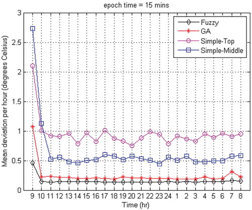
plots the average deviation of the temperature throughout the operating time. The horizontal axis represents time, and the vertical axis represents average temperature deviation in degrees Celsius. The results obtained by the fuzzy control method, Simple-Top, Simple-Middle, and GA-based methods are presented in different colors and plotted using different symbols. Because the fuzzy control method supports fast and dynamic control, the fuzzy control method outperforms all other methods. The deviation is lowest when the fuzzy control is utilized using the proposed fuzzy rules. The deviation at the start time is high because the temperature at the start is higher than the desired temperature.
Figure 5. Average temperature deviation per hour.
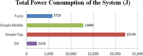
plots the variation of temperature and the power consumption of the system. It reveals the total power consumed by the system. The horizontal axis represents the methods, and the vertical axis represents the total power consumption. The power consumed using the fuzzy method is lower than that consumed using the Simple-Top or Simple-Middle method. It consumed just double that consumed using the GA method, which is the method based on an optimizing algorithm. The proposed method is satisfactory.
Figure 6. Total power consumption of the system.
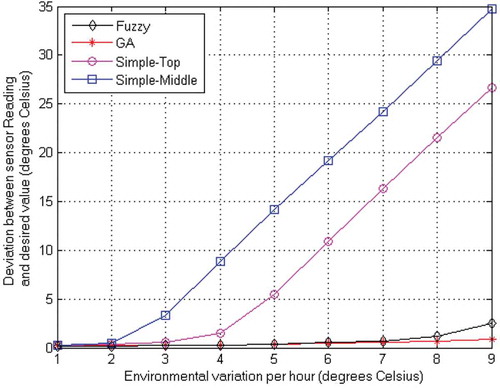
In , the horizontal axis represents the change in environmental temperature per hour, and the vertical axis represents the average temperature deviation of the system. The average temperature deviation dramatically increases with a fast rise in environmental temperature when either the Simple-Top or the Simple-Middle method is used, because only one operator operates in the system. The capability of the operator in Simple-Middle is less than that in Simple-Top. The fuzzy control method, when implemented using our fuzzy rules, performs quite well even if the temperature varies dramatically.
Figure 7. Temperature-deviation variation along with changes in temperature per hour.
Conclusion
Taking into account both the desired reference value and the energy economizing of a cyber-physical system, fuzzy membership functions and fuzzy rules are utilized to achieve this goal. Multilevel data are used to control and determine the decision. The fuzzy control method, implemented using the proposed fuzzy rules, outperforms the other methods in terms of average temperature deviation.
The fuzzy control method is, however, much worse than the GA control method in minimizing the power consumption of the system. In , the fuzzy control method would have used double the energy that the GA control method used. The fuzzy control method is an option for those who care about minimizing deviations of process variables but who have little regard for curtailing power consumption. The epoch of GA deduces the computation of power consumption. An effective means of combining the GA-based method and the fuzzy control method should be sought in the future to improve performance.
References
- Andrei, N. 2005. Modern control theory - A historical perspective. Pennsylvania State University. http://citeseerx.ist.psu.edu/viewdoc/download?doi=10.1.1.134.4498&rep=rep1&type=pdf ( accessed September 8, 2012).
- Aytug, H., and G. J. Koehler. 1996. Stopping criteria for finite length genetic algorithms. Information Journal on Computing 8 (2):183–91.
- Aytug, H., and G. J. Koehler. 2000. New stopping criterion for genetic algorithms. European Journal of Operational Research 126:662–74. doi:10.1016/S0377-2217(99)00321-5.
- Branch, J. W., L. Chen, and B. K. Szymanski. 2008. A middleware framework for market-based actuator coordination in sensor and actuator networks. Paper presented at the International Conference on Pervasive Services, 101–10. Sorrento, Italy, July 6–10.
- Feng, B., G. Gong, and H. Yang. 2009. Self-tuning-parameter fuzzy PID temperature control in a large hydraulic system. Paper presented at the IEEE/ASME International Conference on Advanced Intelligent Mechatronics 1418–22, Singapore, July 14–17.
- Hall, H. R. 1907. Governors and governing mechanisms (2nd ed.). Manchester, England: The Technical Publishing Co.
- Ilić, M. D., L. Xie, U. A. Khan, and J. M. F. Moura. 2010. Modeling of future cyber-physical energy systems for distributed sensing and control. IEEE Transactions on Systems, Man and Cybernetics, Part A: Systems and Humans 40 (4):825–38. doi:10.1109/TSMCA.2010.2048026.
- Li, T. H. S., S. J. Chang, and W. Tong. 2004. Fuzzy target tracking control of autonomous mobile robots by using infrared sensors. Fuzzy Systems 12 (4):491–501. doi:10.1109/TFUZZ.2004.832526.
- Liu, Z., D. Yang, D. Wen, W. Zhang, and W. Mao. 2011. Cyber-physical-social systems for command and control. IEEE Intelligent Systems 26 (4):92–96. doi:10.1109/MIS.2011.69.
- Monzingo, R. A., and T. W. Miller. 1980. Introduction to adaptive arrays. New York, NY: John Wiley & Sons.
- Poovendran, R. 2010. Cyber–physical systems: Close encounters between two parallel worlds. Proceedings of the IEEE 98 (8):1363–66. doi:10.1109/JPROC.2010.2050377.
- Rosenblueth, A., N. Wiener, and J. Bigelow. 1943. Behavior, purpose and teleology. Philosophy of Science 10 (1):18–24. doi:10.1086/phos.1943.10.issue-1.
- Sharapov, R. R., and A. V. Lapshin. 2006. Convergence of genetic algorithms. Pattern Recognition and Image Analysis 16 (3):392–97. doi:10.1134/S1054661806030084.
- Stankovic, J., C. Lu, S. Son, and G. Tao. 1999. The case for feedback control real-time scheduling. Paper presented at the Proceedings of the 11th Euromicro Conference on Real-Time Systems, 11–20. York, England, June 9–11.
- Wolf, W. 2009. Cyber-physical systems. IEEE Computer 42 (3):88–89. doi:10.1109/MC.2009.81.
- Xia, F., Y. Sun, and Y. C. Tian. 2009. Feedback scheduling of priority-driven control networks. Computer Standards & Interfaces 31 (3):539–47. doi:10.1016/j.csi.2008.03.020.