GVSEE: A Global Village Service Effort Estimator to Estimate Software Services Development Effort

ABSTRACT

As software services have become a main and basic part of companies in recent years, accurate and efficient estimates of required effort for their development has turned into a major concern. Furthermore, the great variety, complexity, nonnormality, and inconsistency of software services have made estimation of the needed development effort a very difficult task. In spite of the numerous studies conducted, and improvements made, in the past, no single model has yet been introduced that can reliably estimate the required effort. All the proposed methods enjoy suitable performance under specific conditions but lack satisfactory accuracy in a general and global space. Therefore, apparently, it is impossible to introduce a global and efficient model for all types of services. This article proposes a new model called GVSEE that emphasizes the idea “Think locally, act globally.” Unlike previous studies, this model does not rely on a specific method and, in addition to combining methods, takes a local look at each software service with the help of fuzzy clustering. The model was evaluated on the real dataset ISBSG and on two artificial datasets, and results obtained indicate its tangible efficiency and the lack of accuracy of other models. As well as its greater accuracy, other advantages of the proposed model over other models are its adaptability and flexibility in confronting complexities and uncertainties present in the area of software services.

Introduction

Software service needs to be studied at greater length as a new and widely applied concept in various computer domains such as cloud computing and Web2 (Hashemi and Razzazi 2011). Unfortunately, the term service has different applications and meanings in different contexts. However, as defined by Limam and Boutaba (2010), a software service is software that is introduced through a browser. The required effort to develop a software service is one of the most important parameters in project management, and its estimation is difficult because of three main reasons: the high variety of services, the great changes in customer demands, and the gap between the hardware and software worlds (Jones 2007). Estimation of the effort required to develop a software service plays a vital role in the success and failure of a project and substantially influences management issues such as scheduling, planning, and budgeting. Therefore, considering the position of the related company and the sensitivity of effort estimation, researchers have been trying for years to introduce efficient and accurate methods and models for estimating the effort required to develop software services (Bardsiri and Hashemi 2014).

Software services have various aspects, and estimation models show how these aspects influence the amount of the required effort. Aspects such as the development team, the service size, the service granularity and its complexity, and variety and lack of sufficient standards have been reasons why less attention has been devoted to the issue of estimating a software service development effort (Tansey and Stroulia 2007). The emphasis of this article is on efforts made to develop software services, and lateral concepts such as hardware, architecture, infrastructure, operating system, and platform are ignored. All estimation methods can be divided into six groups:

1. Expert judgment such as the Delphi technique and the Work Breakdown Structure (WBS) (Dejaeger et al. 2012),

2. Machine learning techniques including artificial neural networks (ANN) and analogy-based estimation (ABE) (Wen et al. 2012),

3. Regression including OLS, Step-Wise Regression (SWR), Multiple Linear Regression (MLR), and the Classification and Regression Trees (CART) method (Nassif, Ho, and Capretz 2013),

4. Algorithmic models such as Software LIfecycle Management (SLIM), Constructive Cost Model (COCOMO), and Software Evaluation and Estimation of Resources - Software Estimation Model (SEER-SEM) (Kocaguneli, Menzies, and Keung 2013),

5. Dynamic models, and finally,

6. Hybrid models such as Localized Multi-estimator (LMES) (Bardisiri, Jawawi, Bardsiri et al. 2013).

Contrary to other project types, such as building houses and producing materials, the special features of software services have made the process of effort estimation more difficult than it seems (Bardsiri and Hashemi 2013). In addition to the intangibility of software services, the various datasets are very heterogeneous and inconsistent. This means that it is impossible to introduce a single model that is suitable for all kinds of services and datasets. To reduce this problem, recent studies have used clustering of software services for localization and for reduction of heterogeneity (Bettenburg, Nagappan, and Hassan 2012; Bardisiri, Jawawi, Bardsiri et al. 2013). Moreover, some articles have explored the idea that the constructed models are not sufficient for all datasets (Azzeh 2012; Menzies et al. 2011). Furthermore, studies have been conducted on combining models, weighting the features of the related project, and weighting the answers obtained from each model (Hsu and Huang 2011; Bardisiri, Jawawi, Hashim et al. 2013;Wu, Li, and Liang 2013).

Unfortunately, there is no agreement on a specific and definite model that can give accurate and suitable answers under all conditions and for all types of services. Apparently, it is necessary to put all of the aforementioned types into a general framework in order to take advantage of the strong points and to reduce the drawbacks of each one. In fact, different services require various estimation methods, and this has been overlooked in previous studies. The purpose of this article is to introduce a highly efficient estimation model called the Global Village Service Effort Estimator (GVSEE), which can perform the estimation process under all conditions and for all services. This model will be tested on three completely different datasets, and the inefficiency of other models (11 famous ones) and the high accuracy of GVSEE will be demonstrated.

The rest of the article is organized as follows. Related research is discussed in the next section. “The GVSEE Model” describes the proposed model. “Experimental Design” is explained in the section that follows that, and its results are presented in “Experimental Results.” Results of the research will be discussed in “Improvements in Performance” and validity threats in “Threats to the Validity of the Proposed Model.” The final section deals with conclusions and future work.

Related Works

In recent decades, software and web engineers have recognized the importance of realistic estimation of the effort required in developing software services. Accurate estimation of this required effort in the early stages of developing the software service substantially helps the project manager in managing and controlling the budget and resources (Trendowicz and Jeffery 2014).

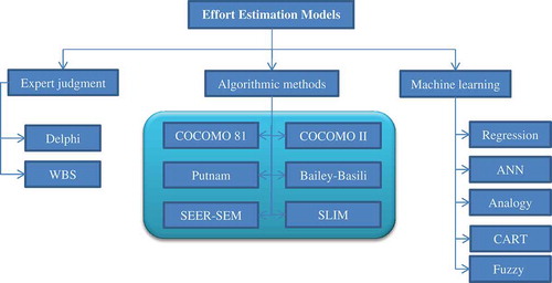
Many techniques have been introduced in the past years to estimate the required effort and cost for developing a software service. As shown in Figure 1, these techniques can be divided into three general groups:

1. Expert judgment: In this method, which was proposed in the late 1960s (Dalkey and Helmer 1963) and is still widely employed in various software companies, domain experts are asked to give their opinions on the required effort. Various amounts are expressed and, typically, their median is returned as the final required effort. The Delphi method is an example of this class of techniques (Moløkken-Østvold and Jørgensen 2004).

2. Algorithmic models: These models, which use mathematical relations and equations, seek to discover a relationship between service attributes and the required effort, are usually suitable for specific cases, and are adjusted and calibrated depending on the existing conditions. COCOMO, SLIM, SEER-SEM are examples of this type of method (Khatibi and Jawawi 2011).

3. Machine learning: These methods look to construct and study algorithms that can learn from datasets, are applied to inputs of the related problem, and help in the decision making. Fuzzy theory, decision tree, ANN, and regression are examples of this class of methods (Wen et al. 2012).

Figure 1. Classification of various types of models for effort estimation.

Numerous studies have compared and evaluated these methods (Dejaeger et al. 2012; Kocaguneli, Menzies, and Keung 2012), but, considering the number of datasets and the existence of various conditions (such as outliers, number of features, filters, number of samples, etc.), there is no general agreement on any single model being one with greater capabilities.

Moreover, other studies attempted to combine these methods and construct hybrid models (Azzeh 2012; Bardsiri, Jawawi, Bardsiri, et al. 2013; Bardsiri, Jawawi, Hashemi, et al. 2013; MacDonell and Shepperd 2003). In most of these studies, analogy was the basis for the functioning of hybrid models and the Analogy Based Estimation (ABE) method was used due to its simplicity and flexibility (Shepperd and Schofield 1997). ABE and particle swarm optimization (PSO; Bardisiri, Jawawi, Hashim et al. 2013), ABE and Differential Evolution (DE), and ABE and Genetic Algorithm (GA) (Li, Xie, and Goh 2007) are examples of hybrid models. The important point is that these hybrid models were not formed by combining the parts; i.e., each part of the hybrid was an independent and separate unit. Moreover, each hybrid used a different approach for improving estimation accuracy. For example, the ABE_GA and ABE_PSO hybrids weighted the attributes whereas the ABE_Grey (Azzeh, Neagu, and Cowling 2010) hybrid improved the distance function to make a better estimate. A global model must include all these advantages and viewpoints, and all related previous studies must be considered in its construction.

The high complexity and inconsistency of software services resulted in no single model being considered as a global model that was suitable under all conditions. Dolado (2001) reported that none of the algorithmic models could function in the global space and, hence, models with greater flexibility were needed. To solve this problem, two main approaches were developed:

1. weighting the answers given by various methods, and

2. clustering and localized comparison.

In various studies, weighting the answers obtained from the various methods was proposed for solving the problem of model globalization and yielded good results (Li, Xie, and Goh 2007, Bardsiri, Jawawi, Bardsiri, et al. 2013; Bardsiri, Jawawi, Hashemi, et al. 2013). Moreover, clustering and localized comparison became the basis for the functioning of some other models for solving the inconsistency problem (Lin and Tzeng 2010; Kocaguneli, Menzies, and Keung 2012). Obtained results showed that clustering and comparison localization substantially increased the accuracy and efficiency of the models. Despite the suitable results obtained in these studies, these two approaches were not used together in any of the models, and furthermore, the combinations of many of the estimation models were not taken into account. These issues will be dealt with in this article.

Lack of sufficient attention to the localization process (type of clustering and number of clusters) was an important threat in previous research. Contrary to other studies, Khatibi et al. 2013 (Bardisiri, Jawawi, Bardsiri et al. 2013) used clustering in place of fuzzy and mathematical equations (considering the nature of the projects) and achieved remarkable results. However, their method is very difficult for artificial software services and large datasets because feature selection will be objective and not subjective. Therefore, two main points must be considered when constructing a global model:

1. creating an accurate and mathematical process of localization, and

2. selecting and allocating suitable estimation models to local spaces.

A global model suitable for all kinds of services and one that is not limited to a specific domain or field, can be constructed by paying sufficient attention to these two points.

The GVSEE Model

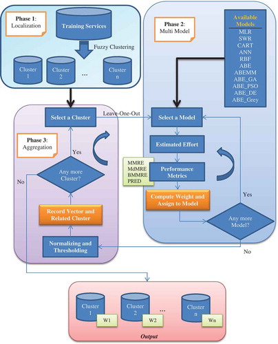
This section explains details of the proposed model. Considering previous research, the main purposes of this model are service localization and estimator combination. The GVSEE model consists of the following three parts.

1. Phase 1 (localization): Clustering of the samples using the fuzzy approach and recognizing similar services.

2. Phase 2 (multimodeling): Using several different estimation models and evaluating them separately on clusters obtained in Phase 1.

3. Phase 3 (aggregation): Aggregating and collecting the answers and weighting all estimation models separately for each cluster.

In the first phase, the samples are divided into several separate clusters based on the degree of similarity and through using fuzzy clustering (Benala et al. 2012). This is actually comparison localization. In the second phase, the most popular models in the three classes of expert, algorithmic, and machine learning are evaluated in local areas to select the best ones among them to prevent dependence on a specific estimation model. In the third phase, these answers are weighed based on performance criteria (explained in “Experimental Design”) and, while thresholding and normalizing, each cluster is allocated a vector of weights. The sequential performance of these three phases will result in a real and efficient comparison. Although each of these elements was used separately in previous studies, to the best of our knowledge, they were never combined together. Selecting one estimator for each cluster, and selecting several estimators for the entire instances, are both unsuitable ideas. Therefore, in GVSEE, both ideas are used together to raise the efficiency. In fact, the idea of “Think locally, act globally” is clearly utilized in the proposed model (Hashemi, Razzazi, and Teshnehlab 2008).

Training Stage

Classification

It has been proved that estimation in a large and global space will not be accurate or efficient, and that the idea of localization must be considered (Bettenburg, Nagappan, and Hassan 2012, Bardsiri, Jawawi, et al. 2013a; Menzies et al. 2013; 2011). Clustering, which will be performed with the help of classic fuzzy clustering, is the first step in building the GVSEE model. This type of clustering was frequently used in previous studies (Benala et al. 2012; Bardsiri, Jawawi, et al. 2013a). The important point in this method is the selection of a suitable number of clusters because it will greatly influence the obtained results.

The main purpose in this phase is to eliminate, or reduce, inconsistencies among the instances so that the most similar services are in one cluster and the instances in different clusters are as different from each other as possible. In this article, the Fuzzy Clustering Method (FCM) method was used because, compared to the k-means method, it more accurately reduces intracluster variance in the clusters and functions. The final goal in this method is to reduce the objective function in Equation (1):

(1)

In the above equation, N and C are the number of instances and clusters, respectively, Uij is the membership degree of Xi in the j cluster and has a value between 0 and 1, Cj is the center of the j cluster, and || is the measured similarity between X and the cluster center. The exact and effective number of clusters depends on data conditions and data type, and a fixed number cannot be considered; however, the number of clusters is calculated based on the algorithm in Figure 18 to prevent optional selection.

The result obtained from the algorithm (Figure 18) depends on data conditions, and the best answer is found by dividing the number of instances by the number of attributes of each instance. Obviously, the level of heterogeneity among the instances and the number of instances will greatly influence the result. Figure 2 is a general view of the training stage in GVSEE, which takes place in three phases.

Figure 2. Training Stage of the GVSEE model.

Multimodeling

As previously mentioned, using a single model will not yield good estimation results. Another goal of GVSEE is to combine several estimation models for each separate cluster. In this article, 11 different estimation models in the three main algorithmic, machine learning, and expert domains were used. Each model was evaluated using the “leave-one-out” technique (on each cluster) and the results were obtained in the format of performance criteria. In fact, the 11 models were evaluated and tested on each cluster derived from Phase 1. In the leave-one-out technique, which is the best and most correct statistical method for validating answers (Kocaguneli and Menzies 2013), in each iteration one service is considered the testing service and the others the training services, and the final answer is calculated through iteration and by averaging all of the services. The weight of each model is then calculated according to Equation (2) and based on the performance criteria (“Experimental Results”).

(2)

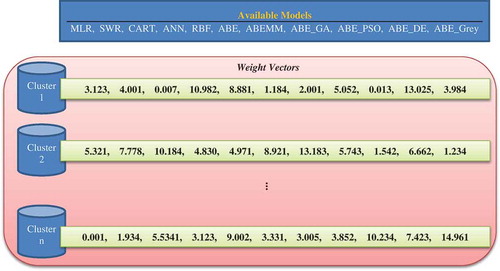
In fact, the output of this phase is n weight vectors for one of the 11 estimators, where n represents the number of clusters. Figure 3 shows an example of the output of this phase. Now, each of the 11 estimators will be separately and briefly explained.

Figure 3. An example of the multi-modeling phase output.

ABE

Shepperd introduced this method in 1997 as a nonalgorithmic method (Shepperd and Schofield 1997), and it has been widely used for estimating required effort. ABE, in which each service is compared with similar previous ones to estimate the required effort, enjoys great simplicity and flexibility, searches the items present in the historical data with the help of a similarity function and a solution function, and returns the closest answer. The first function is employed for finding the degree of similarity and the second for generating an answer.

CART

The purpose in CART is to build a structured decision tree for classifying the set of instances in the dataset. The partition criterion is the simple testing of the features of the instances, and the tree is built recursively using simple if–then rules (Breiman et al. 1984). Each instance, depending on the values of its features, moves on the tree and reaches a specific leaf (which, here, is the amount of effort). This model was used in some of the previous studies (Benala et al. 2014; Dejaeger et al. 2012; Bardsiri, Jawawi, Bardsiri, et al. 2013; Bardsiri, Jawawi, Hashemi, et al. 2013; Zhang, Yang, and Wang 2015).

SWR and MLR

Regression methods are among the oldest estimation methods and try to fit a function to a set of data. The dataset includes a dependent variable E and several independent variables Xi, and the linear Equation (3) is considered for the data (Bardsiri, Jawawi, Bardsiri, et al. 2013; Bardsiri, Jawawi, Hashemi, et al. 2013; Bardsiri et al. 2014):

(3)

In this equation, B is the slope of the line and b the value of the intercept, which can obviously be obtained by adding the one’s column to the X vector In regression models, the purpose is to find the B and b coefficients in such a way that error is minimized. MLR and SWR are examples of single and nonhybrid models that are used in GVSEE.

ANN and RBF

The neural network is a nonlinear model that imitates the function of the human brain and has frequently been used for estimating effort. The neural network consists of a set of neurons in several layers that transport incoming information on their outgoing connections to other units through weighting and by using a suitable transfer function. To generate the output, the inputs take the weight and bias of each neuron and the transfer function processes the inputs of each neuron (Nassif, Capretz, and Ho 2012; Pillai and Jeyakumar 2015). RBF is a special type of ANN that has an input layer, a hidden layer with several neurons, and a Gaussian transfer function. This network is in the form of three forward layers and a linear outgoing layer (Dejaeger et al. 2012).

ABE_Grey and ABEMM

As was previously mentioned, the ABE method, various forms of which have been introduced, uses the two main functions of similarity and solution to estimate effort. ABEMM is a version of ABE that uses the similarity function Manhattan and the solution function Median (Azzeh 2012), and the Grey version employs the Grey theory and measurement of the similarity of two instances is based on fuzzy concepts (Azzeh, Neagu, and Cowling 2010). Customization of the two main functions in the ABE method results in the generation of various versions of it, and many instances of this method can be observed in previous studies (Azzeh 2012; Bardisiri, Jawawi, Hashim et al. 2013; Bardsiri et al. 2014; Shepperd and Schofield 1997).

ABE_GA, ABE_PSO and ABE_DE

The efficiency of the ABE method has been enhanced with the help of optimization algorithms and methods such as DE, PSO, and GA have been employed for weighting the Similarity function (Li, Xie, and Goh 2007; Bardisiri, Jawawi, Hashim et al. 2013). This weighting of attributes makes the comparison process more accurate and completely defines the importance of each feature. The weights found in the training stage (with the help of optimization algorithms) will be used to estimate the required effort for a new service.

Aggregation

In this phase, output vectors of the previous stage are first normalized and then the threshold value is applied to them. In the normalization step, the weights are placed in the [0, 1] interval by using Equation (4) to prepare the input for the thresholding step.

(4)

In this equation, is the weight of the ith model and and are the maximum and minimum weights of each vector, respectively. After normalization, weights of less than 0.3 are omitted in the thresholding stage to ignore models that have little influence so that their high level of error does not have a negative effect on the result returned by GVSEE. Equation (5) indicates how thresholding of weight vectors is performed. In this equation, is the weight of the ith model.

(5)

Selection of more powerful models and omission of the weak results of other models will lead to very accurate effort estimates being made by the cluster. In general, the output of the training stage of GVSEE is a set of clusters together with the weight vector of each cluster.

The Testing Stage

In this stage, the required effort for the development of each service is determined with the help of the clusters and the weights obtained in the training stage. In fact, the services are divided into several clusters in the training stage and the best weight combination of the models is found for each cluster. Figure 4 is a schematic representation of the testing stage.

Figure 4. The testing stage of GVSEE.

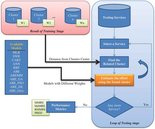
The first step in this stage for each service is to find a suitable cluster based on the distance of the new service from the centers of the clusters. The new service is allocated to the cluster, the center of which is the shortest distance from the service. The models in the cluster are then used to estimate the effort required for the service, and the weights are applied according to Equation (6). In this equation, Wi is the weight of the ith model and the effort estimated by the ith model. This process is repeated for all test services and, in the end, performance criteria of the testing stage are calculated.

(6)

Experimental Design

Datasets

A dataset must be used to construct and evaluate various effort-estimation models. Previous studies used different datasets, and a thorough review of their features and accuracies are presented in Mair, Shepperd, and Jørgensen (2005). In this section, three different datasets are used, two of which are artificial and one is real. A description of each dataset follows.

ISBSG

The International Software Benchmarking Standard Group (ISBSG) is an Australian-based company that collects information on software projects from all over the world. The ISBSG 11 version includes 5052 software projects, each with 109 features (ISBSG 2011). The data covers a broad spectrum of operating systems, programming languages, and development tools. Figure 5 is the graphic representation of the process of applying the filters.

Figure 5. The filtering process on the ISBSG dataset.

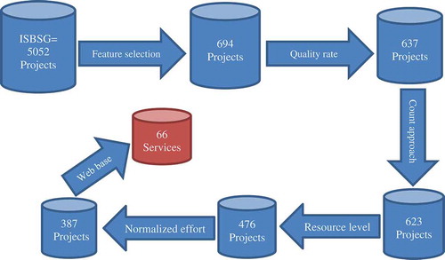
Filters, including those mentioned following, have been developed to work with the data (this subset was selected by reviewing previous studies, and the ISBSG company itself recommended it):

1. Data with the quality rates of a and b

2. Only web-based projects (the software service concept)

3. Identical measurement method for all projects International Function Point Users Group (IFPUG)

4. Selection of six of the more important features that influence the amount of effort

5. Normalization ratio of less than 1.2

6. Resource level less than 1 (to avoid efforts not related to developing the service)

Finally, when all these conditions are applied, 66 software services are obtained. The statistical information of these software services are presented in Table 1. All evaluations are then performed using these 66 services.

Table 1. Description of ISBSG dataset.

Variable	Minimum	Maximum	Mean	Median	Std
InpCont	3	1185	169	95	199
OutCont	10	698	143	67	165
EnqCont	3	653	150	116	137
FileCont	7	384	129	108	97
IntCont	5	497	76	43	95
AFP	107	2245	672	507	534
NorEffort	562	60826	6860	4899	8406

Artificial Datasets

Unfortunately, real datasets are often old and small with a large number of outliers. Therefore, we are forced to use artificial data to test models. Pickard, Kitchenham, and Linkman (2001) introduced a method for generating simulated data. Equation (7) shows the basis of their method (and so do Ahmed, Omolade Saliu, and AlGhamdi 2005 and Li, Xie, and Goh 2009).

(7)

IN this equation, , , and are independent variables obtained from the gamma random distribution of the variables x́₁, x́₂, and x́₃ (with a mean of 4 and variance of 8). The next variable is a relative error calculated from the following equation.

(8)

In this equation, e is the random error resulting from the normally distributed random variable with a mean of zero and a variance of 1, and finally, c is a constant. An artificial dataset has the three main features of variance, skewness, and outlier; and two different types of datasets are obtained depending on the values of these three features. Values of the outliers are obtained through multiplication and division of a percentage of the data by specific constant values. Table 2 shows the adjustments made in the two artificial datasets and the values related to them.

Table 2. Description of artificial datasets’ parameters.

Dataset	Relative error constant	Outlier constant	Outliers percentage
Moderate	0.1	2	5%
Severe	6	6	10%

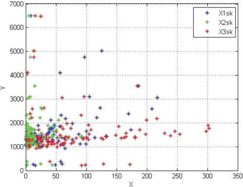
Figures 6 and 7 indicate scatter plots of the 100 data items produced by the datasets Severe and Moderate, respectively. The presence of scattered and deviant values resulting from random distribution causes estimates made by artificial datasets also to be difficult and accompanied by error, so that they can be used in constructing and evaluating models.

Figure 6. Y versus X values of artificial Moderate dataset.

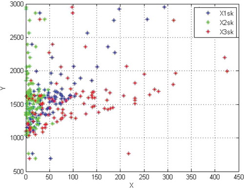
Figure 7. Y versus X of artificial Severe dataset.

Performance Criteria

Many different performance criteria have been introduced in various articles. In this research, five different performance criteria are used. The purpose in using these criteria is to assess the estimation accuracy of the models. For example, absolute residual (AR) shows the difference and gap between actual and estimated values according to Equation (9) (Shepperd and Schofield 1997).

(9)

In this equation, and are the actual and the predicted values, respectively, of the ith instance. Magnitude of relative error (MRE) is an accepted, important, and extensively used performance criterion in effort estimation. As shown in Equation (10), MRE is the error rate between the actual required effort and the estimated one. Lower MRE values indicate better model performance (Shepperd and Kadoda 2001).

(10)

Two other important criteria that are obtained from the overall mean and median of errors are presented in Equations (11) and (12), respectively. Here also, lower values signify better model performance. The difference between the two parameters mean magnitude of relative error (MMRE) and median magnitude of relative error (MdMRE) is that the median is less sensitive to large values and to outliers. The PRED(0.25) parameter, which is the percentage of successful predictions that fall within 25% of the actual values, is a usual substitute for MMRE and is expressed in Equation (13). For example, PRED(0.25) = 0.5 means that half of the estimates have a 25% distance from the actual values.

(11)

(12)

(13)

The next performance criterion is Balanced MMRE (BMMRE), which was introduced by Foss et al. (2003) and is defined in Equation (14). Because the MMRE and MdMRE criteria might lead to asymmetric results, this balanced criterion is used as a substitute. All these criteria must be as small as possible except for PRED(0.25), which must be maximized. Therefore, in “Related Works,” the PRED-(MMRE+MdMRE+BMMRE) function (that must be as large as possible) was used for weighting. The aforementioned criteria were selected because they were extensively used in previous works on effort estimation. A detailed discussion of performance criteria is beyond the scope of this article, and so we will use the most popular ones.

(14)

Preliminary Adjustments

Identical datasets were prepared for all estimation models in the previous section and, in this section, special adjustments are dealt with that are required for each model. Preliminary adjustments are extensive for some models but slight for others.

MLR, SWR, and CART

Because the MLR, SWR, and CART methods, and most regression models, have problems with values of categorical attributes, the optimal scaling technique (Angelis, Stamelos, and Morisio 2001) is used to solve this problem. These models and methods were frequently used in previous studies.

ANN

A two-layer feed forward neural network can be used to approximate a broad spectrum of linear and nonlinear equations. Here, nine neurons are used and the Tan-sigmoid transfer function is employed. There are 300 iterations in order to obtain better results. Previous works on estimating required effort are used to adjust the values in the neural network (Park and Baek 2008; Shukla, Shukla, and Marwala 2014).

RBF

Here also, the maximum number of neurons is nine, and the network output is the estimated required effort to develop the service. RBF is a three-layer feed forward network with one input layer and several neurons, including radial Gaussian transfer functions. The number of iterations depends on the full training of the network and on the addition of all of the neurons.

ABE

As previously mentioned, the ABE model uses the two functions of similarity and solution to estimate the required effort. Here, the similarity function yields the Euclidean distance and the solution function yields the inverse distance weighted mean (Kadoda et al. 2000; Shepperd and Schofield 1997). Moreover, it is assumed there are three similar services (KNN = 3). Various configurations were used so that we could obtain the best structure.

ABE_GA, ABE_PSO, and ABE_DE

In this type of hybrid models, the best ABE structure (described in the previous section) is selected, and optimization algorithms create weights in the [0, 1] interval for the features in the similarity function. This will make the comparison process much more accurate. In all three algorithms, the number of the population is 30, the iteration number is 100, and the fitness function is (MMRE+MdMRE+BMMRE)-PRED (which must be minimized). Table 3 presents partial information on each of these algorithms. References Bardsiri, Jawawi, Bardsiri, et al. (2013), Bardsiri, Jawawi, Hashemi, et al. (2013), and Li, Xie, and Goh (2007) contain studies conducted on these methods and on their applications.

Table 3. Description of algorithms’ parameters.

Algorithm	Parameters
DE	Crossover rate = 0.1
	F Constant = 2
	Schema = DE/Best/1
PSO	C1 = C2 = 2
	W = 1
GA	Crossover rate = 0.7
	Mutant rate = 0.3
	Elite number = 3
Population size = 30, Number of iterations = 100 Fitness function = (MMRE+MdMRE+BMMRE)-PRED

Implementation

The powerful MATLAB software was used to conduct an empirical study because it contains most mathematical functions, neural networks, and decision and clustering trees in its toolbox. Moreover, independent models such as PSO, DE, ABE and their versions were separately implemented. It must be noted that the process of evaluating various models was performed iteratively and randomly using the leave-one-out technique. The predefined functions newff, train, sim, and newrb were used for constructing and training neural networks, and the fcm function was employed for fuzzy clustering. The genetic toolbox in MATLAB was used for implementing the GA algorithm, the eval function for evaluating regression models and the decision tree, and finally, the 3-fold technique for dividing the data into the training and testing sections.

Experimental Results

Results Obtained on ISBSG

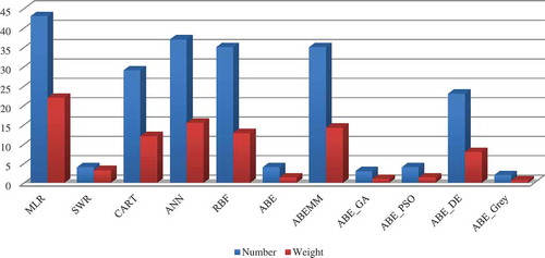
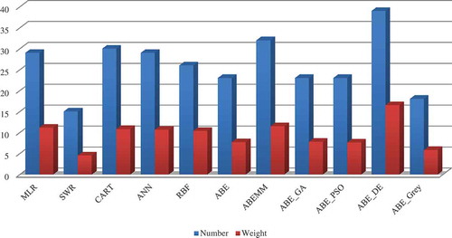
The GVSEE model performs clustering according to the algorithm in Figure 18, and, considering that the 3-fold validation technique is used, we will have different options for each model that is present in GVSEE. Here, n is the number of runs and m the number of clusters. Figure 8 shows the number of times GVSEE selects each of the various models and the weight of each model. The weight of a model means how much it influences the ultimate result. The number of times a model is selected is different from its weight, and a model may have little influence on the ultimate result even if it is selected, and vice versa.

Figure 8. Selection frequencies of the various estimation models present in the ISBSG.

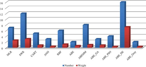
As can be seen in this figure, ABE_DE, SWR, and ABEMM were the first to third most frequently selected models (in the order written), and the ABE_Grey model was the least frequently selected. From 20 possible selections, AB_DE was selected 16 times and ABE_Grey only twice. These results are completely dependent on the type of dataset used.

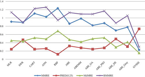
Table 4 lists performance criteria obtained, with the help of the 3-fold technique, from various estimation models present in the ISBSG dataset. These criteria include MMRE, MdMRE, BMMRE, and PRED(0.25).

Table 4. Performance criteria of the ISBSG dataset in the various estimation models.

	Train				Test
Models	MMRE	PRED(0.25)	MdMRE	BMMRE	MMRE	PRED(0.25)	MdMRE	BMMRE
MLR	0.7535	0.3539	0.3622	0.9263	0.909	0.2438	0.4517	1.1369
SWR	0.7065	0.3032	0.3501	0.9245	0.8927	0.4705	0.4370	0.8874
CART	0.8320	0.2536	0.5293	1.3137	1.1077	0.2453	0.5198	1.2271
ANN	0.8082	0.3692	0.4154	0.9775	1.0258	0.259	0.4913	1.2595
RBF	1.0409	0.2380	0.5138	1.8857	1.2345	0.1219	0.6857	0.9444
ABE	0.8863	0.3301	0.4269	1.1515	0.8606	0.3225	0.4747	1.1293
ABEMM	0.6858	0.3227	0.3656	0.9866	0.986	0.2770	0.4204	1.0937
ABE_GA	0.9280	0.2686	0.4398	1.2216	0.8196	0.2453	0.4977	1.0930
ABE_PSO	0.8492	0.2612	0.4520	1.1196	0.8745	0.2763	0.5205	1.1670
ABE_DE	0.6431	0.4150	0.3356	0.8425	0.6966	0.4927	0.2928	0.8770
ABE_Grey	0.8361	0.2922	0.4630	1.1763	0.7779	0.3073	0.4166	1.0557
GVSSE	0.3296	0.5827	0.2317	0.4378	0.2272	0.7359	0.1538	0.2961

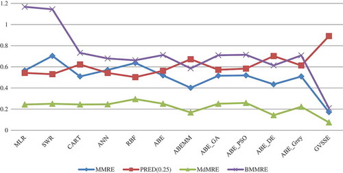
As results in the table indicate, the proposed model yielded more accurate and better results than all other models in both the training and the testing stages. The largest PRED(0.25) and the smallest MMRE, MdMRE, and BMMRE belong to GVSEE. Figure 9 is a graphic representation of the test stage for the four performance criteria and of the various estimation models. As can be seen in this figure, next to GVSEE, ABE_DE yielded the best and RBF the worst answers.

Figure 9. The testing results of different models on ISBSG dataset.

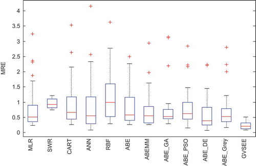
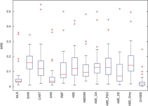
Because performance criteria are cumulative and general, an accurate statistical tool is needed to show details of how estimation errors are distributed. Boxplot is a kind of graph that can indicate the median, distribution, and range of values well. Moreover, Figure 10 shows the boxplot diagram related to the MRE of various models. This diagram demonstrates the way errors are distributed in various estimation models. As shown in Figure 10, the inter-quartile distance in GVSEE is shorter than other models, and the smallest median is obtained from GVSEE. Moreover, the number of outliers in GVSEE is the smallest among the models. Next to the proposed model, the SWR method yielded the best and the RBF the worst answers.

Figure 10. The Box diagram of MRE distribution in the various models present in ISBSG.

Results on the Moderate Dataset

Here, also, the 3-fold validation technique was employed and, because the number of instances was greater, more clusters were formed compared to the ISBSG dataset. Figure 11 shows the selection frequency and the degree of influence of each model for 50 different runs. This figure is, in fact, the result of multiple runs of the training stage of the GVSEE model.

Figure 11. Selection frequencies and weights of various estimation models on the Moderate dataset.

As seen in the figure, MLR was selected most frequently and had the greatest influence with ANN, ABEMM, and RBF, respectively, following. The worst answers were those of the ABE_Grey method. Obviously, these results are different from those of the ISBSG dataset and depend on the nature of the services. MLR was the most frequently selected (43 times) and ABE_Grey the least frequently (2 times). Moreover, the weighting models such as ABE_DE, ABE_PSO, and ABE_GA did not yield acceptable results on the Moderate dataset. Table 5 shows performance criteria obtained from various effort-estimation models in the training and testing stages. Figure 12 is a graphic representation related to the testing stage of various effort-estimation models.

Table 5. Performance criteria of various models in the artificial Moderate dataset.

	Train				Test
Models	MMRE	PRED(0.25)	MdMRE	BMMRE	MMRE	PRED(0.25)	MdMRE	BMMRE
MLR	0.0531	0.9599	0.0233	0.0631	0.0650	0.9598	0.0342	0.0746
SWR	0.1203	0.8808	0.0197	0.1429	0.1363	0.7718	0.0929	0.1956
CART	0.1374	0.8798	0.0676	0.1596	0.1442	0.8499	0.0832	0.1685
ANN	0.0521	0.9599	0.0228	0.0652	0.0690	0.9598	0.0329	0.0786
RBF	0.0822	0.9350	0.0364	0.0969	0.1120	0.8695	0.0627	0.1475
ABE	0.1127	0.8600	0.0436	0.1344	0.1443	0.8196	0.0875	0.1759
ABEMM	0.1004	0.9099	0.0516	0.1224	0.1232	0.8998	0.0733	0.1495
ABE_GA	0.1165	0.8649	0.0515	0.1400	0.1443	0.8196	0.0880	0.1732
ABE_PSO	0.1138	0.8699	0.0504	0.1362	0.1467	0.8003	0.0860	0.1804
ABE_DE	0.0926	0.9199	0.0316	0.1137	0.1118	0.9096	0.0495	0.1331
ABE_Grey	0.1222	0.8349	0.0531	0.1545	0.1586	0.7896	0.0918	0.2039
GVSSE	0.0818	0.9608	0.0222	0.0646	0.0323	0.9696	0.0075	0.0455

Figure 12. The testing results of different models on artificial Moderate dataset.

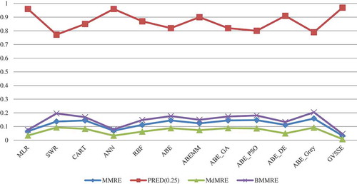
As seen in the figure, GVSEE had the least MMRE, MdMRE, and BMMRE values compared to the other models, and it produced the largest PRED(0.25). The two methods SWR and ABE_Grey performed the worst. Considering the low heterogeneity of this dataset and its artificial nature, all the results obtained here are relatively suitable and there is little difference among the models. The boxplot diagram in Figure 13 indicates the way MRE values were distributed for the various effort-estimation models. Here also, the least median and interquartile belonged to the proposed model and, next to it, MLR and ANN had suitable error distribution and small medians. Considering the larger number of services in this dataset, a greater number of outliers can be seen in the boxplot diagram. This figure shows how various models estimate and indicates their efficiencies well.

Figure 13. The Boxplot diagram of MRE distribution in various models in the Moderate dataset.

Results on the Severe Dataset

In this section, the last dataset (which was constructed artificially but with high heterogeneity) is evaluated. Figure 14 shows selection frequencies of various estimation models and the weight of each model in the ultimate result. These results were obtained from 40 possible selections and from multiple runnings of the training stage of the GVSEE model.

Figure 14. Selection frequencies and weights of various estimation models on the Severe dataset.

As seen in the figure, the ABE_DE model enjoyed the highest number of selections followed by ABEMM and CART, respectively. The lowest number of selections was that of the SWR model. Here, the models have a suitable balance and frequency of selections because the dataset is heterogeneous, and hence, clusters face completely different conditions. ABE_DE and SWR were the most and the least frequently selected models with 39 and 15 selections, respectively. Table 6 lists the performance criteria related to the various models in the training and testing stages on the Severe dataset.

Table 6. Performance criteria of various models in the artificial Severe dataset.

	Train				Test
Models	MMRE	PRED(0.25)	MdMRE	BMMRE	MMRE	PRED(0.25)	MdMRE	BMMRE
MLR	0.5154	0.5756	0.2120	0.6151	0.5652	0.5427	0.2437	1.1679
SWR	0.6777	0.4500	0.3931	0.9249	0.7035	0.5303	0.2506	1.1442
CART	0.6355	0.5555	0.2208	0.8513	0.5092	0.6224	0.2440	0.7324
ANN	0.5251	0.5508	0.2310	0.6209	0.5704	0.5424	0.2453	0.6793
RBF	0.5060	0.4806	0.2643	0.6537	0.6366	0.5023	0.2955	0.6621
ABE	0.5226	0.5807	0.2031	0.6952	0.5188	0.5632	0.2513	0.7118
ABEMM	0.4010	0.6903	0.1250	0.5971	0.4020	0.6720	0.1680	0.5855
ABE_GA	0.5452	0.5410	0.2277	0.7138	0.5156	0.5724	0.2510	0.7098
ABE_PSO	0.3340	0.5759	0.2148	0.7150	0.5194	0.5834	0.2589	0.7142
ABE_DE	0.4953	0.6257	0.1736	0.6496	0.4344	0.7020	0.1425	0.6136
ABE_Grey	0.5709	0.5707	0.2135	0.7426	0.5093	0.6131	0.2229	0.7084
GVSSE	0.2001	0.7385	0.1129	0.5810	0.1716	0.8912	0.07468	0.2093

Figure 15 is the graphical representation of the testing stage in Table 6. Clearly, contrary to the Moderate dataset, here, the solution interval is varied and different. GVSEE yielded by far the best answers (PRED(0.25) the largest, and MMRE, MdMRE, and BMMRE the smallest), and SWR the worst answers, of all of the parameters. The BMMRE parameter, by its definition, had the broadest range of changes and showed the differences well in the performance of various estimation models.

Figure 15. The testing results of different models on artificial Severe dataset.

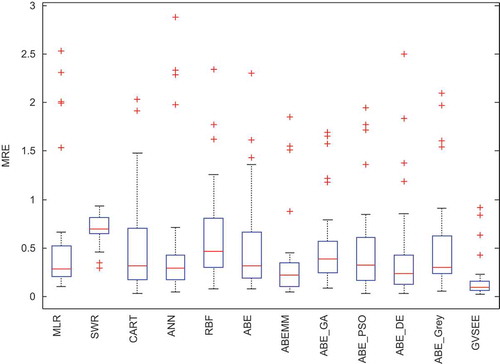
Figure 16 uses the boxplot diagram to prevent biased comparison of the way errors are distributed. In this diagram, tangible differences can be seen between GVSEE and other models, because GVSEE has a much lower interquartile and a very small median, whereas CART and ABE have broad interquartile ranges and greater medians than GVSEE. Moreover, considering the high level of heterogeneity and the large number of services, there are many outliers in this diagram. By using each specific estimation model in its unique position (identified in the training stage), GVSEE raised the efficiency well and created differences. In the next section, statistical improvements and comparison of GVSEE’s performance with those of other estimation models will be presented.

Figure 16. The Boxplot diagram of MRE distribution in various models in the Severe dataset.

Improvements in Performance

Experimental results of the previous section showed that the proposed model fundamentally improved performance criteria. Moreover, statistical diagrams suggest GVSEE results are more accurate than other estimation models. Because the proposed model is supported by the three main ideas of clustering, multimodeling, and aggregating, its good performance was predictable. Results showed one important message: various effort-estimation models perform completely differently and an overall view to datasets will not yield good results. In the section on model selection, we noticed that a model could be excellent for a specific part of the dataset but completely unsuitable for other parts. The motto of GVSEE is “Think locally, act globally.” The improvement value of different models is calculated using Equation (15) where shows the best result of independent model for each evaluation criterion and shows the outcome of the proposed model for the same corresponding criterion.

(15)

Tables 7–9 indicate percentage improvement in various performance criteria on the three datasets ISBSG, Moderate, and Severe, respectively. In each column of the tables, the greatest and smallest improvements are indicated by max and min, respectively.

Table 7. Percentage of improvement obtained by GVSEE on ISBSG dataset.

Method Metric	MMRE	PRED(0.25)	MdMRE	BMMRE
MLR	75.00	201.84max	65.95	73.95
SWR	74.54	56.40	64.80	66.63
CART	79.48	200.00	70.41	75.86
ANN	77.85	184.13	68.69	76.49max
RBF	81.59max	503.69	77.57max	68.64
ABE	73.59	128.18	67.60	73.78
ABEMM	76.95	165.66	63.41	72.92
ABE_GA	72.27	200.00	69.09	72.90
ABE_PSO	74.01	166.34	70.45	74.62
ABE_DE	67.38min	49.36min	47.47min	66.23min
ABE_Grey	70.79	139.47	63.08	71.95

Table 8. Percentage of improvement obtained by GVSEE on Moderate dataset.

Method Metric	MMRE	PRED(0.25)	MdMRE	BMMRE
MLR	50.24min	1.02min	77.85	38.97min
SWR	76.24	25.62max	91.84max	76.70
CART	77.54	14.08	90.88	72.96
ANN	53.12	1.021	77.01min	42.08
RBF	71.10	11.51	87.90	69.11
ABE	77.56	18.30	91.33	74.09
ABEMM	73.72	7.75	89.66	69.52
ABE_GA	77.56	18.30	91.38	73.69
ABE_PSO	77.92	21.15	91.18	74.74
ABE_DE	71.03	6.59	84.70	65.77
ABE_Grey	79.58max	22.79	91.74	77.65max

Table 9. Percentage of improvement obtained by GVSEE on Severe dataset.

Method Metric	MMRE	PRED(0.25)	MdMRE	BMMRE
MLR	69.63	64.21	69.35	82.07max
SWR	75.60max	68.05	70.19	81.70
CART	66.30	43.18	69.39	71.42
ANN	69.91	64.30	69.55	69.18
RBF	73.04	77.42max	74.72max	68.38
ABE	66.92	58.23	70.28	70.59
ABEMM	57.31min	32.61	55.54	64.25min
ABE_GA	66.71	55.69	70.24	70.51
ABE_PSO	66.96	52.75	71.15	70.69
ABE_DE	60.49	26.95min	47.59min	65.88
ABE_Grey	66.30	45.35	66.49	70.45

As shown in Table 7, the minimum improvement for the MMRE criterion is 67% and belongs to the ABE_DE method and the maximum 81% is that of RBF. For the PRED(0.25) criterion, the improvement values are very large and tangible because, here, the services enjoy great variety. As for the MdMRE criterion also, the least improvement of 47% is that of the ABE_DE method, and finally, the BMMRE criterion enjoyed a minimum improvement of 66%. Therefore, GVSEE fundamentally improved the criteria and obtained results were completely different.

Table 8 indicates that improvement was tangible and substantial for all of the criteria except for PRED(0.25) (because of the nature of the Moderate dataset and its homogeneity), and that most models yielded suitable answers, and hence, improvement was in the [1–22]% interval. However, here also, no criterion deteriorated and GVSEE caused improvements, albeit small ones, in all of the criteria. The homogeneity of the Moderate dataset causes the improvements and differences not to be conspicuous. This problem has been solved in the other two datasets (Severe and ISBSG).

Table 9 belongs to the dataset Severe that, due to its high level of heterogeneity and because of the variety of its services, shows the differences well. Here, among all the various models and performance criteria, the minimum improvement is 26% and the maximum is 82%. The BMMRE parameter enjoys the maximum improvement and, in most models, the answers have improved by more than 50%. This is the result of clustering and is due to the idea of localized estimation because GVSEE selects the estimation method based on the existing conditions.

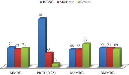
Finally, Figure 17 indicates the mean improvement of each performance criterion in the various datasets. Results suggest fundamental changes in answers and the much higher accuracy of GVSEE. The improvement value of 181% for the PRED(0.25) criterion in the ISBSG dataset results from the great difference in the values of this criterion in the proposed model and in the worst model in this dataset (RBF). Results suggest that GVSEE enjoys the required flexibility and capability for estimating the effort any kind of software service requires, and that it is quite comparable to the best available effort estimation models. Moreover, the values in the tables show the relative improvements of various estimation models in relation to each other, improvements that are very small (about 10%–20%) compared to those in GVSEE. The reasons for this are that, in other models there is an overall look to datasets, and the datasets are not clustered because outliers strongly influence the results of these models. It must be kept in mind that the datasets used are completely different from each other and are of different natures, so they can show the efficiency of the proposed model and its difference from the other methods well.

Figure 17. Mean improvement of each performance criterion in the different datasets.

Threats to the Validity of the Proposed Model

Any research or scientific study can be faced with some internal and external threats. In fact, models must be correctly understood and utilized for their results to be correct and usable. In this section, some of the internal and external threats that GVSEE faces are explained.

Internal Threats

One of the main threats to the validity of an effort estimation model is the question of its correct and accurate evaluation. For example, using a part of the training data for testing the model is a very bad idea because the efficiency that is obtained will not be real. Another bad idea is to consider a fixed number of services for testing the model; the correct thing to do is to use techniques such as fold cross-validation or leave one out, each of which has both the training and the testing roles; and, for this reason, these statistical methods were very frequently used in previous studies.

Another threat is the selection of performance criteria: these criteria must be selected carefully and without bias. In this article, because estimate accuracy was our purpose, we used four of the most popular parameters. Because these criteria are extensively used, their selection allows obtained results to be easily compared with those of other studies and allows us to use statistical tools such as the boxplot diagram that help us see the variance and distribution of the answers.

The next item is the method of constructing the model, that is, how parameters can be adjusted and weighted in adjustable models; for example, what type of similarity and solution functions and what value for KNN should be used. In this article, construction and adjustment of parameters have been described in detail. Of course, different constructions will have numerous adjustments and, hence, various answers. In this article, it was attempted to use the most powerful and popular effort-estimation methods, although GVSEE is sufficiently flexible to include new and better methods and, in fact, is a flexible and open structure.

External Threats

In future studies, the most important external threats will be the way GVSEE will be used and generalized in the real world. All limitations and risks should be considered for the proposed model so that correct results can be obtained. For example, GVSEE is not dependent on any specific dataset and can completely adapt itself to various types of data and services. Moreover, it does not have any specific method for selecting attributes and important instances in a dataset and for filtering them, rather, it performs clustering based on the fuzzy concept.

The term globalization has a somewhat different meaning in software services because here there are high degrees of variety and uncertainty, and proposing a general framework for all kinds of services seems to be impossible. We believe GVSEE has at least raised the range of backup support for all different kinds of services. Inflexibility is an important external threat for any effort-estimation model. As was previously mentioned, GVSEE uses 11 different estimation models, can support more models with great flexibility, and has a completely correctible structure for future use.

The last type of external threat is the question of customized execution and manual operation of the model. Fortunately, most GVSEE models work automatically and do not require any intervention (except for the selection of estimators, which is completely customized).

Conclusion and Future Work

Accurate estimation of effort required for developing a software service plays an essential role in project management. Over- and underestimation waste system resources and endanger the position of the related company. Heterogeneity, nonnormality, and complexity are the main reasons for incorrect estimates in developing services. Moreover, the competitive market and the great variety of software services are the problems various estimation models face. Recent studies on a broad spectrum of models have indicated that no model is the suitable solution for all conditions and that every model works well under some conditions but poorly under others. In fact, the main and fundamental problem for current models is to consider all services in the process of effort estimation. These reasons led to the introduction of a new global model based on the three fundamental principles of clustering services for the purpose of estimate localization, using several instead of one estimation model in order to increase the strong points and decrease the weak points, and aggregating the answers given by the various models. The proposed model uses 11 different effort-estimation methods, utilizing the best performance of each. The real database ISBSG and two artificial databases (Moderate and Severe) were used for evaluating the GVSEE model, and results indicated substantial improvements in performance criteria. The main advantages of GVSEE are that it is not dependent on any specific dataset and that it can be expanded (other methods can be added to it). GVSEE does not depend on a specific set of estimators, rather, it finds the optimal combination of estimators every time (depending on the existing conditions) through the training process. Future research can include the use of newer estimators in the framework of GVSEE and a more accurate clustering process. It can also improve estimator selection by employing new performance criteria.

Figure 18. Determining the number of clusters.

Acknowledgments

We would like to express our gratitude to the ISBSG Company for providing us with its valuable data to conduct this study, and also to the Bardsir Branch of the Islamic Azad University for their moral support.

References

- Ahmed, M. A., M. Omolade Saliu, and J. AlGhamdi. 2005. Adaptive fuzzy logic-based framework for software development effort prediction. Information and Software Technology 47 (1):31–48. doi:10.1016/j.infsof.2004.05.004.
- Angelis, L., I. Stamelos, and M. Morisio. 2001. Building a software cost estimation model based on categorical data. In Proceedings of the seventh international software metrics symposium, METRICS 2001. IEEE.
- Azzeh, M. 2012. A replicated assessment and comparison of adaptation techniques for analogy-based effort estimation. Empirical Software Engineering 17 (1–2):90–127. doi:10.1007/s10664-011-9176-6.
- Azzeh, M., D. Neagu, and P. I. Cowling. 2010. Fuzzy grey relational analysis for software effort estimation. Empirical Software Engineering 15 (1):60–90. doi:10.1007/s10664-009-9113-0.
- Bardsiri, A. K., and S. M. Hashemi. 2013. Electronic services, the only way to realize the global village. International Journal of Mechatronics, Electrical and Computer Technology 3 (6):1039–41.
- Bardsiri, A. K., and S. M. Hashemi. 2014. Software effort estimation: A survey of well-known approaches. International Journal of Computer Science Engineering 3 (1):46–50.
- Bardsiri, V. K., D. N. A. Jawawi, S. Z. M. Hashim, and E. Khatibi. 2013. LMES: A localized multi-estimator model to estimate software development effort. Engineering Applications of Artificial Intelligence 26 (10):2624–40.
- Bardsiri, V. K., D. N. A. Jawawi, A. K. Bardsiri, and E. Khatibi. 2013. A PSO-based model to increase the accuracy of software development effort estimation. Software Quality Journal 21 (3):501–26. doi:10.1007/s11219-012-9183-x.
- Bardsiri, V. K., D. N. A. Jawawi, S. Z. M. Hashim, and E. Khatibi. 2014. A flexible method to estimate the software development effort based on the classification of projects and localization of comparisons. Empirical Software Engineering 19 (4):857–84. doi:10.1007/s10664-013-9241-4.
- Benala, T. R., R. Mall, S. Dehuri, and V. Prasanthi 2012. Software effort orediction using fuzzy clustering and functional link artificial neural networks. In Swarm, evolutionary, and memetic computing. Berlin Heidelberg: Springer.
- Benala, T. R., R. Mall, P. Srikavya, and M. V. HariPriya 2014. Software effort estimation using data mining techniques. In ICT and critical infrastructure: Proceedings of the 48th annual convention of computer society of India-vol I. Switzerland: Springer.
- Bettenburg, N., M. Nagappan, and A. E. Hassan. 2012. Think locally, act globally: Improving defect and effort prediction models. In 9th IEEE working conference on mining software repositories (MSR), 2012. Zurich: IEEE.
- Breiman, L., J. Friedman, C. J. Stone, and R. A. Olshen. 1984. Classification and regression trees. New York: CRC press.
- Dalkey, N., and O. Helmer. 1963. An experimental application of the delphi method to the use of experts. Management Science 9 (3):458–67. doi:10.1287/mnsc.9.3.458.
- Dejaeger, K., W. Verbeke, D. Martens, and B. Baesens. 2012. Data mining techniques for software effort estimation: A comparative study. IEEE Transactions on Software Engineering 38 (2):375–97. doi:10.1109/TSE.2011.55.
- Dolado, J. J. 2001. On the problem of the software cost function. Information and Software Technology 43 (1):61–72. doi:10.1016/S0950-5849(00)00137-3.
- Foss, T., E. Stensrud, B. Kitchenham, and I. Myrtveit. 2003. A simulation study of the model evaluation criterion MMRE. IEEE Transactions on Software Engineering 29 (11):985–95. doi:10.1109/TSE.2003.1245300.
- Hashemi, S. M., and M. Razzazi. 2011. Global village services as the future of electronic services. Saarbrücken, Germany: Lambert Academic Publishing.
- Hashemi, S. M., M. Razzazi, and M. Teshnehlab. 2008. Streamlining the global village grid services. World Applied Sciences Journal 3 (5):824–32.
- Hsu, C.-J., and C.-Y. Huang. 2011. Comparison of weighted grey relational analysis for software effort estimation. Software Quality Journal 19 (1):165–200. doi:10.1007/s11219-010-9110-y.
- ISBSG (2011). International software benchmarking standard group. Data CD Release 11. www.isbsg.org.
- Jones, C. 2007. Estimating software costs: Bringing realism to estimating. New York NY,: McGraw-Hill Companies.
- Kadoda, G., M. Cartwright, L. Chen, and M. Shepperd. 2000. Experiences using case-based reasoning to predict software project effort. Paper presented at the Proceedings of the EASE Conference, Keele, UK, March 2000.
- Khatibi, V., and D. N. A. Jawawi. 2011. Software cost estimation methods: A review Journal of emerging trends in computing and information sciences 2 (1):21–29.
- Kocaguneli, E., and T. Menzies. 2013. Software effort models should be assessed via leave-one-out validation. Journal of Systems and Software 86 (7):1879–90. doi:10.1016/j.jss.2013.02.053.
- Kocaguneli, E., T. Menzies, and J. W. Keung. 2012. On the value of ensemble effort estimation. IEEE Transactions on Software Engineering 38 (6):1403–16. doi:10.1109/TSE.2011.111.
- Kocaguneli, E., T. Menzies, and J. W. Keung. 2013. Kernel methods for software effort estimation. Empirical Software Engineering 18 (1):1–24. doi:10.1007/s10664-011-9189-1.
- Li, Y., M. Xie, and T. Goh. 2007. A study of genetic algorithm for project selection for analogy based software cost estimation. Paper presented at the IEEE International Conference on Industrial Engineering and Engineering Management, Singapore, December 2–4.
- Li, Y.-F., M. Xie, and T. N. Goh. 2009. A study of project selection and feature weighting for analogy based software cost estimation. Journal of Systems and Software 82 (2):241–52. doi:10.1016/j.jss.2008.06.001.
- Limam, N., and R. Boutaba. 2010. Assessing software service quality and trustworthiness at selection time. IEEE Transactions on Software Engineering 36 (4):559–74. doi:10.1109/TSE.2010.2.
- Lin, J.-C., and H.-Y. Tzeng. 2010. Applying particle swarm optimization to estimate software effort by multiple factors software project clustering. Paper presented at the IEEE International Computer Symposium (ICS), Taiwan, December 16–18.
- MacDonell, S. G., and M. J. Shepperd. 2003. Combining techniques to optimize effort predictions in software project management. Journal of Systems and Software 66 (2):91–98. doi:10.1016/S0164-1212(02)00067-5.
- Mair, C., M. Shepperd, and M. Jørgensen. 2005. An analysis of data sets used to train and validate cost prediction systems. ACM SIGSOFT software engineering notes, New York, NY: ACM.
- Menzies, T., A. Butcher, D. Cok, A. Marcus, L. Layman, F. Shull, B. Turhan, and T. Zimmermann. 2013. Local versus global lessons for defect prediction and effort estimation. IEEE Transactions on Software Engineering 39 (6):822–34. doi:10.1109/TSE.2012.83.
- Menzies, T., A. Butcher, A. Marcus, T. Zimmermann, and D. Cok. 2011. Local vs. global models for effort estimation and defect prediction. In Proceedings of the 2011 26th IEEE/ACM international conference on automated software engineering. IEEE Computer Society.
- Moløkken-Østvold, K., and M. Jørgensen. 2004. Group processes in software effort estimation. Empirical Software Engineering 9 (4):315–34. doi:10.1023/B:EMSE.0000039882.39206.5a.
- Nassif, A. B., L. F. Capretz, and D. Ho. 2012. Software effort estimation in the early stages of the software life cycle using a cascade correlation neural network model. Paper presented at the 13th ACIS IEEE International Conference on Software Engineering, Artificial Intelligence, Networking and Parallel & Distributed Computing (SNPD), Kyoto, Japan, August 8–10.
- Nassif, A. B., D. Ho, and L. F. Capretz. 2013. Towards an early software estimation using log-linear regression and a multilayer perceptron model. Journal of Systems and Software 86 (1):144–60. doi:10.1016/j.jss.2012.07.050.
- Park, H., and S. Baek. 2008. An empirical validation of a neural network model for software effort estimation. Expert Systems with Applications 35 (3):929–37. doi:10.1016/j.eswa.2007.08.001.
- Pickard, L., B. Kitchenham, and S. Linkman. 2001. Using simulated data sets to compare data analysis techniques used for software cost modelling. IEE Proceedings-Software 148 (6):165–74. doi:10.1049/ip-sen:20010621.
- Pillai, S., and M. Jeyakumar. 2015. General regression neural network for software effort estimation of small programs using a single variable. In Power electronics and renewable energy systems. India: Springer.
- Shepperd, M., and C. Schofield. 1997. Estimating software project effort using analogies. IEEE Transactions on Software Engineering 23 (11):736–43. doi:10.1109/32.637387.
- Shepperd, M., and G. Kadoda. 2001. Comparing software prediction techniques using simulation. IEEE Transactions on Software Engineering 27 (11):1014–22. doi:10.1109/32.965341.
- Shukla, R., M. Shukla, and T. Marwala. 2014. Neural network and statistical modeling of software development effort. In Proceedings of the second international conference on soft computing for problem solving (SocProS 2012). December 28–30, 2012, India: Springer.
- Tansey, B., and E. Stroulia. 2007. Valuating software service development: integrating COCOMO II and real options theory. In Proceedings of the first international workshop on the economics of software and computation. May 20–26, 2007, Minneapolis, MN: IEEE Computer Society.
- Trendowicz, A., and R. Jeffery. 2014. Principles of effort and cost estimation. In Software project effort estimation. Switzerland: Springer.
- Wen, J., S. Li, Z. Lin, Y. Hu, and C. Huang. 2012. Systematic literature review of machine learning based software development effort estimation models. Information and Software Technology 54 (1):41–59. doi:10.1016/j.infsof.2011.09.002.
- Wu, D., J. Li, and Y. Liang. 2013. Linear combination of multiple case-based reasoning with optimized weight for software effort estimation. The Journal of Supercomputing 64 (3):898–918. doi:10.1007/s11227-010-0525-9.
- Zhang, W., Y. Yang, and Q. Wang. 2015. Using Bayesian regression and em algorithm with missing handling for software effort prediction. Information and Software Technology 58:58–70. doi:10.1016/j.infsof.2014.10.005.