Source Reconstruction of Atmospheric Releases with Limited Meteorological Observations Using Genetic Algorithms

Abstract

A genetic algorithm is paired with a Lagrangian puff atmospheric model to reconstruct the source characteristics of an atmospheric release. Observed meteorological and ground concentration measurements from the real-world Dipole Pride controlled release experiment are used to test the methodology. A sensitivity study is performed to quantify the relative contribution of the number and location of sensor measurements by progressively removing them. Additionally, the importance of the meteorological measurements is tested by progressively removing surface observations and vertical profiles. It is shown that the source term reconstruction can occur also with limited meteorological observations. The proposed general methodology can be applied to reconstruct the characteristics of an unknown atmospheric release given limited ground and meteorological observations.

Introduction

Atmospheric Transport and Dispersion (AT&D) models predict the fate of the contaminant after it is released in the atmosphere and determine the air quality factors that have an impact on health, such as the distribution of contaminant concentration, peak concentrations, dosage, and deposition (Allen et al. 2007b; Cervone and Franzese 2011; Cervone et al. 2010a; Cervone et al. 2010b; Franzese 2003). Several factors affect the dispersion of the contaminants, including the source characteristics, the surrounding topography, and the local micrometeorology.

Source characterization for airborne contaminants is an important criterion to perform air quality analysis. The aim of source characterization is to discover the locations, and strengths and size of one or more sources. Once the origin is identified, releases from the source may be mitigated or, at the very least, modeled to predict their environmental impact. Currently, the technique available for characterizing contaminant sources combine forward-predicting AT&D and backward-looking models (Allen et al. 2007a). The approach presented in this paper couples a forward dispersion model with a genetic algorithm (GA).

Several popular artificial intelligence algorithms use Bayesian inference combined with stochastic sampling (e.g., Chow, Kosovic´, and Chan 2006; Delle Monache et al. 2008; Gelman et al. 2003; Johannesson, Hanley, and Nitao 2004; Senocak et al. 2008). Another approach based on evolutionary computation has also been suggested and tested (e.g., Allen et al. 2007a; Cervone and Franzese 2010b; Haupt, Young, and Allen 2007). Evolutionary computation algorithms (of which GAs are one of the main paradigms, in addition to evolutionary strategy (ES), genetic programming and evolutionary programming) are iterative stochastic methods that evolve in parallel a set of potential solutions (individuals) based on a fitness function. The solutions are encoded as vectors of numbers (binary, integer, or real), which can include a number of source characteristics such as its geometry, size, location, and emission rate. Each solution is evaluated according to an objective function (often referred to as fitness function, cost function, or error function), which is, in general, calculated as the difference between the concentration field simulated by the dispersion model from a generated source, and the real observations. The evolutionary process consists of selecting one or more candidate individuals whose vector values are modified to minimize the fitness function. A selection process is used to determine which of the new solutions survive into the next generation.

This characteristic suits well with the source detection problem, where real-valued attributes are most common. GA and ES converge (De Jong 2008): lately is very common now to encounter GA operating on real-valued parameters such as the continuous parameters illustrated in Haupt (2005); Haupt, Young, and Allen (2007); Allen et al. (2007b) and Long, Haupt, and Young (2010), as well as ES with parallel search streams and even crossover operator (e.g., De Jong 2008).

For example, a GA with continuous parameter was used in the context of a source allocation exercise (Haupt 2005); soil water characteristic curve modeling in unsaturated soils (Ahangar-Asr, Johari, and Javadi 2012); volcanic source inversion (Tiampo et al. 2004); coupled with a Gaussian plume model in a source detection and modeling problem using synthetic data as receptor data (Allen et al. 2007b; Haupt, Young, and Allen 2007); and to assess the sensitivity of a source detection method to the number of sensors (Long, Haupt, and Young 2010). In all the mentioned applications, the ES achieved good results, demonstrating its suitability as optimization technique. An alternative methodology of the evolutionary algorithm approach was proposed by Cervone et al. (2010b) and Lattner and Cervone (2012), where new candidate solutions were created through a process guided by machine learning, rather than the canonical Darwinian operators of mutation and crossover.

The goal of this work is to perform a sensitivity study on the role of meteorological observations and ground concentration with respect to the reconstruction of the source. Real-world data from the Dipole Pride experiment are used, and several tests are performed to determine how much of the meteorological observations and ground concentration measurements are required for an accurate reconstruction of the source characteristics.

Specifically, the GA is used to test and validate two major problems. The first problem is to understand the relative contribution of the number and location of the observed concentration. This sensitivity study consists of utilizing a subset of all the data available, and determining the smallest set of concentrations that are needed for an adequate source reconstruction. The second problem is to understand how much meteorological data are needed for an accurate reconstruction. This involves removing from the computation the meteorological data and the vertical profile.

Data and models

Dipole Pride data

The Dipole Pride field experiments (DP26) were conducted in November of 1996 at Yucca Flat (37 N, 116 W), at the Nevada Test Site, Nevada. The main goal was to validate transport and dispersion models; more details about the experiments are provided in Watson et al. (1998); Biltoft (1998).

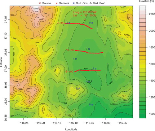
The Dipole Pride experiments consisted in a series of instantaneous releases of sulfur hexafluoride (SF6). Seventeen different field tests were performed under different atmospheric conditions. In this work, the data collected for experiment number 4 are used. This experiment consisted in a sequence of two consecutive releases under similar atmospheric conditions. Figure 1 shows the test domain used for the experiment, the source location, the three rows of receptors, the weather stations, and the vertical profile.

Each row of receptors contains 30 measurements locations (1–30, 31–60, and 61–90). The temporal resolution of the observations is 15 minutes. Additionally, five high temporal resolution (3 seconds) receptors were located along the second row of measurements. These data were not used in the experiments.

Chang et al. (2003a) used the DP26 data experiments to validate various dispersion models, including Second-order Closure Integrated Puff model (SCIPUFF), used in this work. They discovered that significant errors occurred when the simulated puff missed the receptors, probably caused by wind interpolation.

Continuous surface meteorological observations at 15-minute interval were collected over the domain of the experiment at eight different locations. The measurements include wind vectors, temperature, humidity, and dew point. Additionally, a vertical profile was collected at the beginning of each experiment at a location roughly located in the center of the domain (shown with a triangle in Figure 1).

SCIPUFF

The T&D model used in this study is the SCIPUFF, a Lagrangian puff dispersion model that uses a set of Gaussian puffs to represent an arbitrary, three dimensional, time-dependent concentration field Sykes, Lewellen, and Parker (1984); Sykes and Gabruk (1997). SCIPUFF takes as input terrain information (elevation and cover), meteorological data such as wind direction and speed, temperature, humidity and precipitation (surface and vertical profiles if available), and the emission source information.

SCIPUFF can simulate both instantaneous releases (e.g., an explosion) and continuous releases (e.g., smoke from a chimney). For this particular problem, SCIPUFF is run assuming instantaneous emissions.

Methodology

The methodology used here is based on numerical AT&D simulations, ground measurements, and a stochastic GA. The GA is used to iteratively refine an initial random guess by varying the x, y, and z coordinates of the source, source emission rate Q, and source dimensions , and . The score for each candidate solution is a metric of how well the simulated concentrations match the DP26 observations.

Genetic algorithms

GAs are metaheuristic techniques that simulate biological evolution to solve computational optimization problems (e.g., De Jong 2008; Holland 1975). They are particularly suited for real-world applications where the solution space is multi-modal and includes several suboptimal solutions.

These algorithms build consecutive populations of solutions, considered as feasible solutions for a given problem, to search for a solution that gives the best approximation to the optimum for the problem under investigation. To this end, a fitness function is used to evaluate the goodness of each individuals based on selection and reproduction with the intent to create new populations (i.e., generations). Each individual is represented by finite length vector of components called chromosome, and each component, following the genetic anthology, gene. The problem’s chromosome is coded using seven continuous variables (, , Q, , , and ). The process of these algorithms is composed by the following steps:

• P₁: a random initial population is generated and a fitness function is used to assign a score to each solution;

• P₂: according to their fitness score, some solutions are selected to form the parents, and new solutions are created by applying genetic operators (i.e., crossover and mutation). For instance, the crossover operator combines two solutions (i.e., parents) to form one or two new solutions (i.e., offspring), while the mutation operator is used to randomly modify a solution. Then, to determine which individuals will survive among the offspring and their parents, a survivor selection is applied according to the solutions’ fitness values;

• P₃: step P₂ is repeated until stopping criteria hold.

The evolutionary process we experimented with employed two widely used selection operators, i.e., roulette wheel and tournament selector. We used the first one to choose the solutions for reproduction, while we employed the tournament selector to determine the solutions that are included in the next generation (i.e., survivals). The former assigns a roulette portion to each solution according to its fitness score. In this way, even if candidate solutions with a higher fitness have higher chance of selection, there is still a chance that they may be not. On the contrary, applying the tournament selector, only the best n solutions (usually ) are copied straight into the next generation.

Crossover and mutation operators were defined to preserve well-formed values in all offspring. To this end, a single-point crossover has been used, which randomly selects the same point in each solution taking the first part of the chromosome (four genes of seven) from the first parent and the second part (three remaining genes) from the second parent. Regarding the mutation, has been applied an operator that selects a gene of the solution and changes it with a random one in a feasible range. Crossover and mutation rates were fixed at 0.5 and 0.2, respectively (Allen et al. 2007a). The evolutionary process is stopped when there is no improvement for a fixed number of consecutive iterations, which means that the 50 individuals converged to a stationary point.

To cope with the random nature of the GA, we performed 30 runs for a statistical study.

We used an implementation of a GA for the R statistical environment, provided through the genalg library.

Fitness function

Central to every evolutionary algorithm is the definition of the error function, often called fitness or objective function. The fitness function evaluates each candidate solution quantifying the error between the observed data and the corresponding simulated one. This information is used by the search algorithm to drive the iterative process.

The definition of error, or uncertainty, in the model predictions is not univocal, and depending on the case, different metrics to evaluate the accuracy of a dispersion calculation can be adopted (Hanna, Chang, and Strimaitis 1993). For instance, the error may represent the comparison of simulated and observed peak concentrations over the entire sensor network, regardless of time and location of occurrence of the peak. In other cases, the only realistic expectation is to calculate the predictions that fall within a certain factor (e.g., 2 or 10) of the observations. For this reason, inter-model comparison studies always include evaluation of different performance metrics (e.g., Cervone and Franzese 2010b; Chang et al. 2003b; Chang and Hanna 2004; Chang et al. 2005).

In this study, the AHY2 function has been used as fitness indicator, defined by Allen et al. (2007b) as suitable to quantify the difference between observed and simulated concentrations for source detection algorithms:

where is each sensor’s observed mean concentration, is the corresponding simulated value, and the horizontal bar represents the average over all the observations.

To test the distance error between the parameters of the real source and the “best” individual from the GA, the Euclidean distance has been used between the best chromosome (lowest fitness) and the Dipole Pride source.

where is the vector of parameters for the observed source and for the simulated one .

Experiments and results

A series of experiments were performed to test the ability of SCIPUFF to reconstruct the source, and a sensitivity study to the number and locations of receptors, as well as to the number and locations of meteorological data.

Baseline source reconstruction

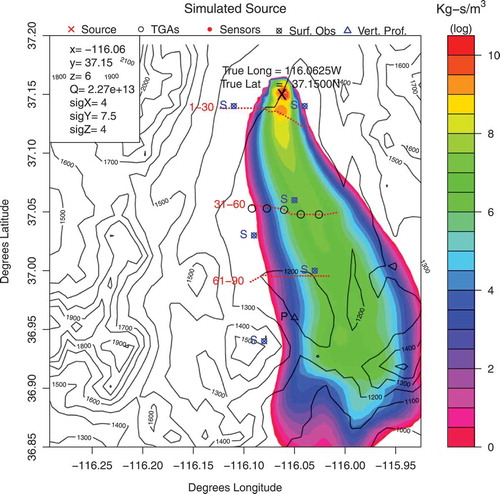
Figure 2 shows the result of the optimization that achieved the smallest error between simulated and observed values. The real source characteristics measured at the time of the experiment are: x = −116.06E, y = 37.15 N, z = 6 m, Q = 2.27E+13 kg-s/, =4 m, =7.5 m, =4 m.

Figure 1. Map for the domain of the Dipole Pride experiment. The source location is indicated with an X, along with its longitude and latitude coordinates. Locations for receptors and meteorological measurements (surface and vertical profile) are also indicated.

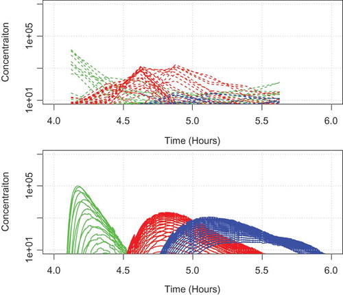
Figure 3 compares the observed (top) to the simulated (bottom) values for the baseline source reconstruction. Each line indicates a sensor measurements (total 90 sensors), and is color-coded according to the rows. Green color lines indicate the first row of sensors, red lines are for the second row, and blue lines for the third row.

Figure 2. Baseline SCIPUFF reconstruction of the source using the characteristics measured at the time of the experiments, and all meteorological data available. Sensor locations and meteorological stations (surface + vertical profile) are also shown.

The top panel of Figure 3 shows the observed values collected at 15-minute interval. The bottom panel of Figure 3 shows the simulated values at 3-second interval. The graph shows a good temporal correlation between simulated and observed values with respect to the first (green) and second (red) rows of measurements. The blue lines, which represent the third row of measurements, are nearly absent in the observations.

Figure 4 (left) shows the concentrations (in log scale) of the baseline simulated release as a function of time in hours (horizontal axis) and space (vertical axis), represented by the three rows of 30 sensors each. Sensors 1–30 are those closest to the source and sensors 61–90 are those farther away (see Figure 1). The figure shows how the gas concentrations spread over time and space. It takes about 10 minutes for the gas to reach the first row, 30 minutes for the second row of measurements, and an additional 30 minutes (1 hour from the initial release) to reach the third row. Overall, it takes more than 4 hours for the concentration measurements to fall below measurable thresholds.

Figure 3. Comparison of observed (top) and simulated (bottom) values for the baseline source reconstruction. Each line indicates a sensor measurement (total 90 sensors), and is color-coded according to the rows. Green color lines indicate the first row of sensors, red lines are for the second row, and blue lines for the third row.

Figure 4 (right) shows the concentrations (in log scale) of the observed values. The observed values are much coarser than the simulated values because the model simulations are run at a 3-second intervals, while the observed values are only 15-minute averages.

Figure 4. Spread of the released gas as a function of space (vertical axis: location of sensors) and time (horizontal axis: elapsed time in hours) for the baseline simulation (left) and using the field measurements (right). Simulations are run with a 3-second time step, while observations are averages of 15 minutes, explaining the coarser representation of observed measurements.

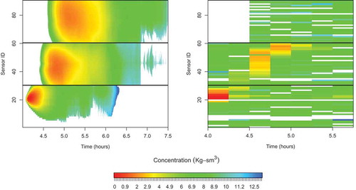
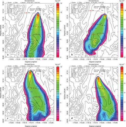
Figure 5. (a) Best run using the weather station numbers 2 and 5 without vertical profile, (b) Best run using the weather station numbers 5 and 7 without vertical profile, (c) Best run using all the weather station numbers without vertical profile, and (d) Best run using all the weather station numbers including the vertical profile.

Despite the mismatch in resolution, there is consistency in space and time between simulated and observed values, especially with respect to the first and second rows of measurements. It appears that the release spread more to the West of the domain that the simulation reconstructs. The error computed when all available data are used is summarized in Figure 2 and Table 1

Table 1. Average error and standard deviation obtained using different sensor measurements combinations.

	90 sensors	First line	Second line	Third line	9 sensors	5 sensors
	13.51	27.8	26.7	42.9	21.3	30.5
SD	±10.59	±20.41	±17.64	±30.89	±16.19	±22.13

Results represent the average of 30 runs of the GA.

Table 2. Error and standard deviation over 30 runs for each experiment.

Metro Stations
1	2	3	4	5	6	7	8	V. Prof.	x	y	z	Q				Avg error	Std error	Avg Dist source	Std Dist source	Avg fitness	Std fitness
Real Source									−116.0625	37.1500	6.0000	2.271911E+13	4.00	7.50	4.00	0.00	0.00	0.00 (0.00 km)	0.00	0.82	0.00
0	0	0	0	1	0	1	0	0	−115.9506	37.1587	10.7680	9.588026E+13	2.07	3.34	4.71	10.99	8.48	0.066 (7.39 km)	0.016	0.82	0.41
0	1	0	0	1	0	0	0	0	−116.0170	37.1227	4.74075	9.526302E+13	5.52	5.45	7.03	12.84	10.19	0.037 (4.11 km)	0.018	0.86	0.30
0	0	0	0	1	0	0	0	0	−115.9785	37.1691	10.0499	9.327056E+13	4.33	7.98	4.73	13.87	12.13	0.070 (7.78 km)	0.022	1.12	0.49
1	1	1	1	1	1	1	1	1	−116.0629	37.1424	10.9563	9.028692E+13	4.27	4.51	2.12	14.68	11.18	0.018 (3.55 km)	0.013	0.82	0.06
1	1	1	1	1	0	1	1	0	−116.0682	37.0781	8.86905	6.237862E+13	4.34	3.00	3.02	14.89	10.00	0.060 (6.67 km)	0.016	0.72	0.26
0	1	0	0	1	0	1	0	0	−116.0406	37.1099	0.52251	9.256595E+13	2.63	4.05	7.68	16.25	11.92	0.044 (4.89 km)	0.014	0.70	0.16
1	1	0	1	1	0	1	0	0	−116.0413	37.0745	5.39974	5.851380E+13	6.96	6.90	3.84	16.51	12.29	0.051 (5.67 km)	0.016	0.66	0.15
1	1	1	1	1	1	1	1	0	−116.1013	37.1679	20.0416	9.813896E+13	7.17	5.81	3.09	17.75	11.36	0.033 (3.66 km)	0.017	0.68	0.15
0	1	0	1	1	0	1	0	0	−116.0152	37.1784	44.9899	9.688432E+13	3.97	6.64	4.12	17.98	13.60	0.055 (6.11 km)	0.014	0.65	0.16
0	1	0	0	0	0	0	0	0	−116.0804	37.1339	44.4615	7.802687E+13	4.98	5.50	6.18	18.97	12.57	0.042 (4.67 km)	0.020	0.70	0.12
1	1	1	1	1	1	1	0	0	−116.1053	37.1693	46.4181	9.205014E+13	3.00	6.45	5.53	19.54	11.35	0.035 (3.89 km)	0.017	0.83	0.58
1	1	0	0	1	0	1	0	0	−116.0004	37.1764	49.2814	8.241115E+13	5.30	2.03	6.35	19.95	13.48	0.046 (5.11 km)	0.016	0.81	0.38
1	1	1	1	1	0	1	0	0	−116.0548	37.0723	4.78756	7.197588E+13	7.62	2.21	5.81	22.09	12.55	0.046 (5.11 km)	0.021	0.74	0.20
0	1	0	1	1	0	0	0	0	−116.0499	37.1082	35.3168	9.582855E+13	2.57	4.091	5.80	20.55	12.43	0.049 (5.44 km)	0.020	0.66	0.14

The 1 in the position means that the weather station i has been used in the experiment j, 0 otherwise. The same is for the vertical profile

Sensitivity to number and location of observations

A series of experiments were performed to test the ability of the proposed methodology to reconstruct the source characteristics with a diminishing number of data. The first set of tests was designed to test the sensor number and locations, and it is described below.

The second set of test is designed to test the number and location of the surface meteorological measurements and of the vertical profile, and is described in the next section.

Eight different receptor subsets are tested:

• all 90;

• the first line (see Figure 3);

• the middle receptor line;

• the last line;

• three sensors for line taken equidistant;

• five sensors taken equidistant on the middle line receptor;

• removing the vertical profile;

• taking only two weather station.

Table 1 summarizes all the results obtained, where each value represents the average of 30 runs. The best source reconstruction (−116.05E, 37.16 N, 23.06 m, 8.16E+13 kg-s/m³, 6.97 m, 7.28 m, 3.68 m, error = 13.51) is found when all 90 sensor receptors are used (all three rows). When only individual rows of sensors are used, best results are obtained using the second row of sensors (error = 26.7), followed by slightly inferior results using the first row of sensors (error = 27.8). Much inferior results are obtained using the third row of sensors (error = 42.9).

Two additional tests are run selecting nine and five random sensors in the second row of sensors. The results show that using 9 sensors, the error is only slightly inferior to when all 30 sensors in the row are used (error 21.3 vs 26.8). However, when only 5 sensors are used, the results degrade to an error of 30.5.

The results show that when using either five or nine random sensors selected among those in the second row, the error is significantly better than when using the third row alone. This result can be explained with the previously discussed observation that the third row of sensors failed to measure significant concentration levels.

Sensitivity to meteorological stations

The second set of tests focuses on determining the sensitivity of the proposed methodology to varying meteorological data. The DP26 experiment includes meteorological data for eight surface stations distributed throughout the domain. Additionally, co-located with meteorological station number 4, a vertical profile is collected at the beginning of each experiment by deploying a weather balloon (see Figure 1).

The experiments were designed to test the sensitivity of the GA methodology to the meteorological observations. The source reconstruction was performed using all 90 ground sensors, and with different combinations of surface meteorological stations and toggling the use of the vertical profile.

Table 2 summarizes the results for all the experiments performed. Each result shows the average result for 30 runs.

As it can be seen in Table 2, the results are compared under three characteristics, the average error over all the GA components (x, y, z, Q, , , ), the average error over the distance from the real source (x, y), and the average fitness evaluated by the GA.

For the first one, the results show that the best combination is using the weather stations 5–7, these two stations are in the exact line of the sensors and in the same way of the original plume, the second best score is achieved by the combination 2–5, and these are the closest stations to the source and are providing a good accuracy for the simulation.

The experiment involving all the weather stations plus the vertical profile (Figure 5d) achieved the forth position, and without the vertical profile (Figure 5c) the eighth position with increments of 20.91% of the error.

An interesting point is given with the worst combination (2-4-5), and this result shows how a single station (far away, in this case, from the source), combined with other good stations could totally bias the research of the real source. When only stations #2 and #5 are used, results show a large error and poor performance. However, when stations #2 and #5 are used in combination (Figure 5a), the results are near optimal, showing lack of accuracy when the stations are tested individually.

The results in terms of average distance from the source show that the best match is obtained when all the stations and the vertical profile are used. The second best match is obtained using the same combination but without the vertical profile. The error expressed in km is between 3.66 and 7.78 over an area of . This result shows the importance of the location of the sensors. The absence of the vertical profile leads to an overall increase in the error. However, the decision to minimize the use of the vertical profile was made because it is usually not available for accidental releases.

Conclusions

This paper shows the importance of the number and locations of meteorological observations and ground concentration required to reconstruct the source characteristics of an unknown pollutant. Experiments were performed using the SCIPUFF T&D model and observations from the Dipole Pride experiment. A traditional GA was used to drive the optimization process. Results show that there is close correlation between the available data and the error, in particular when data characterizing the atmosphere’s vertical profile are omitted. The results are particularly important for the determination of how many sensors and their locations should be deployed when planning for release experiments.

This work also indicates a sensitivity to meteorological data that are available. It is not possible to assume that data at one point in space and time adequately represent the meteorological conditions over the region, which can vary widely. Prior work showed that one approach is to include the wind speed and direction in the search variables, which can produce better agreement with measurements than assuming that the meteorological data are representative of the entire domain (Allen et al. 2007b; Krysta et al. 2006).

Funding

Work performed under this project has been also partially funded by the Office of Naval Research (ONR) award #N00014-14-1-0208 (PSU #171570).

Additional information

Funding

Work performed under this project has been also partially funded by the Office of Naval Research (ONR) award #N00014-14-1-0208 (PSU #171570).

References

- Ahangar-Asr, A., A. Johari, and A. A. Javadi. 2012. An evolutionary approach to modelling the soil–water characteristic curve in unsaturated soils. Computers and Geosciences 43:25–33. doi:10.1016/j.cageo.2012.02.021.
- Allen, C. T., S. E. Haupt, and G. S. Young. 2007a. Source characterization with a genetic algorithm-coupled dispersion-backward model incorporating scipuff. Journal of Applied Meteorology and Climatology 46 (3):273–87. doi:10.1175/JAM2459.1.
- Allen, C. T., G. S. Young, and S. E. Haupt. 2007b. Improving pollutant source characterization by better estimating wind direction with a genetic algorithm. Atmospheric Environment 41 (11):2283–89. doi:10.1016/j.atmosenv.2006.11.007.
- Biltoft, C. A. 1998. Dipole pride 26: Phase ii of defense special weapons agency transport and dispersion model validation. Technical report, DTIC Document, Defense Technical Information Center.
- Cervone, G., and P. Franzese. 2010a. Machine learning for the source detection of atmospheric emissions. Proceedings of the 8th Conference on Artificial Intelligence Applications to Environmental Science, Number J1.7, January.
- Cervone, G., and P. Franzese. 2010b. Monte Carlo source detection of atmospheric emissions and error functions analysis. Computers and Geosciences 36 (7):902–09. doi:10.1016/j.cageo.2010.01.007.
- Cervone, G., and P. Franzese. 2011. Non-darwinian evolution for the source detection of atmospheric releases. Atmospheric Environment 45 (26):4497–506. doi:10.1016/j.atmosenv.2011.04.054.
- Cervone, G., P. Franzese, and A. Grajdeanu. 2010a. Characterization of atmospheric contaminant sources using adaptive evolutionary algorithms. Atmospheric Environment 44:3787–96. doi:10.1016/j.atmosenv.2010.06.046.
- Cervone, G., P. Franzese, and A. P. Keesee. 2010b. Algorithm quasi-optimal (AQ) learning. Wires: Computational Statistics 2 (2):218–36.
- Chang, J. C., P. Franzese, K. Chayantrakom, and S. R. Hanna. 2003a. Evaluations of calpuff, hpac, and vlstrack with two mesoscale field datasets. Journal of Applied Meteorology 42 (4):453–66. doi:10.1175/1520-0450(2003)042<0453:EOCHAV>2.0.CO;2.
- Chang, J. C., P. Franzese, K. Chayantrakom, and S. R. Hanna. 2003b. Evaluations of CALPUFF, HPAC, and VLSTRACK with two mesoscale field datasets. Journal of Applied Meteorology 42 (4):453–66. doi:10.1175/1520-0450(2003)042<0453:EOCHAV>2.0.CO;2.
- Chang, J. C., and S. R. Hanna. 2004. Air quality model performance evaluation. Meteorology and Atmospheric Physics 87:167–96. doi:10.1007/s00703-003-0070-7.
- Chang, J. C., S. R. Hanna, Z. Boybeyi, and P. Franzese. 2005. Use of Salt Lake City Urban 2000 field data to evaluate the Urban Hazard Prediction Assessment Capability (HPAC) dispersion model. Journal of Applied Meteorology 44 (4):485–501. doi:10.1175/JAM2205.1.
- Chow, F., B. Kosovic´, and T. Chan. 2006. Source inversion for contaminant plume dispersion in urban environments using building-resolving simulations. Proceedings of the 86th American Meteorological Society Annual Meeting, Atlanta, GA, 12–22.
- De Jong, K. 2008. Evolutionary computation: A unified approach. Proceedings of the 2008 GECCO Conference on Genetic and Evolutionary Computation, ACM, New York, NY, USA, 2245–58.
- Delle Monache, L., J. Lundquist, B. Kosovic´, G. Johannesson, K. Dyer, R. Aines, F. Chow, R. Belles, W. Hanley, S. Larsen, G. Loosmore, J. Nitao, G. Sugiyama, and P. Vogt. 2008. Bayesian inference and markov chain monte carlo sampling to reconstruct a contaminant source on a continental scale. Journal of Applied Meteorology and Climatology 47:2600–13. doi:10.1175/2008JAMC1766.1.
- Franzese, P. 2003. Lagrangian stochastic modelling of a fluctuating plume in the convective boundary layer. Atmospheric Environment 37:1691–701. doi:10.1016/S1352-2310(03)00003-7.
- Gelman, A., J. Carlin, H. Stern, and D. Rubin. 2003. Bayesian data analysis, 668. Chapman & Hall/CRC: London, UK.
- Hanna, S. R., J. C. Chang, and G. D. Strimaitis. 1993. Hazardous gas model evaluation with field observations. Atmospheric Environment 27A:2265–85. doi:10.1016/0960-1686(93)90397-H.
- Haupt, S. E. 2005. A demonstration of coupled receptor/dispersion modeling with a genetic algorithm. Atmospheric Environment 39 (37):7181–89, December. doi:10.1016/j.atmosenv.2005.08.027.
- Haupt, S. E., G. S. Young, and C. T. Allen. 2007. A genetic algorithm method to assimilate sensor data for a toxic contaminant release. Journal of Computers 2 (6):85–93, August. doi:10.4304/jcp.2.6.85-93.
- Holland, J. 1975. Adaptation in natural and artificial systems. Cambridge, MA: The MIT Press.
- Johannesson, G., B. Hanley, and J. Nitao. 2004. Dynamic Bayesian Models via Monte Carlo - An introduction with examples. Technical Report UCRL-TR-207173, Lawrence Livermore National Laboratory, October.
- Krysta, M., M. Bocquet, B. Sportisse, and O. Isnard. 2006. Data assimilation for short-range dispersion of radionuclides: An application to wind tunnel data. Atmospheric Environment 40 (38):7267–79. doi:10.1016/j.atmosenv.2006.06.043.
- Lattner, A. D., and G. Cervone. 2012. Ensemble modeling of transport and dispersion simulations guided by machine learning hypotheses generation. Computers and Geosciences 48:267–79. doi:10.1016/j.cageo.2012.01.017.
- Long, K. J., S. E. Haupt, and G. S. Young. 2010. Assessing sensitivity of source term estimation. Atmospheric Environment 44 (12):1558–67. doi:10.1016/j.atmosenv.2010.01.003.
- Senocak, I., N. Hengartner, M. Short, and W. Daniel. 2008. Stochastic event reconstruction of atmospheric contaminant dispersion using Bayesian inference. Atmospheric Environment 42 (33):7718–27. doi:10.1016/j.atmosenv.2008.05.024.
- Sykes, R. I., and R. S. Gabruk. 1997. A second-order closure model for the effect of averaging time on turbulent plume dispersion. Journal of Applied Meteorology 36:165–84. doi:10.1175/1520-0450(1997)036<1038:ASOCMF>2.0.CO;2.
- Sykes, R. I., W. S. Lewellen, and S. F. Parker. 1984. A turbulent transport model for concentration fluctuation and fluxes. Journal Fluid Mechanisms 139:193–218. doi:10.1017/S002211208400032X.
- Tiampo, K., J. Ferna´Ndez, G. Jentzsch, M. Charco, and J. Rundle. 2004. Volcanic source inversion using a genetic algorithm and an elastic-gravitational layered earth model for magmatic intrusions. Computers and Geosciences 30 (9):985–1001. doi:10.1016/j.cageo.2004.07.005.
- Watson, T., R. Keislar, B. Reese, D. George, and C. Biltoft. 1998. The defense special weapons agency dipole pride 26 field experiment. NOAA Air Resources Laboratory Tech. Memo. ERL ARL-225.