DAG Scheduling in Heterogeneous Computing and Grid Environments Using Variable Neighborhood Search Algorithm

ABSTRACT

DAG scheduling is a process that plans and supervises the execution of interdependent tasks on heterogeneous computing resources. Efficient task scheduling is one of the important factors to improve the performance of heterogeneous computing systems. In this paper, an investigation on implementing Variable Neighborhood Search (VNS) algorithm for scheduling dependent jobs on heterogeneous computing and grid environments is carried out. Hybrid Two PHase VNS (HTPHVNS) DAG scheduling algorithm has been proposed. The performance of the VNS and HTPHVNS algorithm has been evaluated with Genetic Algorithm and Heterogeneous Earliest Finish Time algorithm. Simulation results show that VNS and HTPHVNS algorithm generally perform better than other meta-heuristics methods.

Introduction

Grids enable the sharing, selection, and aggregation of a wide variety of heterogeneous resources including supercomputers, storage systems, data sources, and specialized devices that are geographically distributed and owned by different organizations. The grid allows users to solve larger-scale problems by pooling together resources that could not be coupled easily before (Foster and Kesselman 2004; Freund and Siegel 1993).The efficiency of executing applications on grid and heterogeneous systems critically depends on the methods used to schedule the tasks onto the processors. Scheduling in grid systems is a challenging task, as it involves coordinating multiple computational sites for resource sharing and scheduling in an efficient manner. Given an application modeled by the Directed Acyclic Graph (DAG), the scheduling problem deals with mapping each task of the application onto the available heterogeneous systems in order to minimize makespan (Chitra, Rajaram, and Venkatesh 2011). DAG includes the characteristics of an application program such as the execution time of tasks, the data size to communicate between tasks, and task dependencies.

Grid and heterogeneous computing systems are exclusively meant for handling large volumes of computational loads such as data generated in the high-energy nuclear physics experiments (Wong et al. 2003), bioinformatics (Darling, Carey, and Feng 2003), and astronomical computations. These applications demand new strategies for collecting, sharing, transferring, and analyzing the data (Viswanathan, Veeravalli, and Robertazzi 2007). Also, those applications have long execution times, and hence they require high-quality task schedules to minimize their run times. Additionally, the static scheduling time of several scientific and engineering applications is much lower than their run time on grid and heterogeneous systems. For example, the execution times of more than 50% of the parallel applications that were run on four real parallel computing systems are between tens and thousands of minutes (Iosup et al. 2006), while the static scheduling times of parallel applications with diverse characteristics, which were scheduled using several static scheduling algorithms, are lower than 1 second (Topcuoglu, Hariri, and Wu 2002). Also, the high throughput of grid and heterogeneous computing systems depends on the efficiency of the scheduling algorithms, which are developed for them (Mohammad and Kharma 2011). However, it is easy to demonstrate that the best existing scheduling algorithms for grid and heterogeneous computing systems generate suboptimal task schedules (Mohammad and Kharma 2008; Sih and Lee 1993; Topcuoglu, Hariri, and Wu 2002). This paves the path to contribute in these lines of research for the development of better scheduling algorithms for the grid and heterogeneous computing systems, able to deal with large-size real-world application scheduling problem instances by using innovative concepts.

The task scheduling problem has been solved several years ago and is known to be NP-complete (Coffman 1976; El-Rewin and Lewis 1990; Garey and Johnson 1979; Ilavarasan, Thambidurai, and Mahilmannan 2005; Kwok and Ahmad 1996, 1999; Sih and Lee 1993; Topcuoglu, Hariri, and Wu 2002; Ullman 1975). In general, task scheduling algorithm for heterogeneous systems is classified into two classes: static and dynamic (Hamidzadeh, Kit, and Lija 2000; Kwok and Ahmad 1999; Zomaya, Ward, and Macey 1999). In static scheduling algorithms, all information needed for scheduling such as the structure of the parallel application, the execution times of individual tasks, and the communication costs between tasks must be known in advance (Mohammad and Kharma 2008, 2011). Static task scheduling takes place during compile time before running the parallel application. In contrast, scheduling decisions in dynamic scheduling algorithms are made at run time. The objective of dynamic scheduling algorithms includes not only creating high-quality task schedules, but also minimizing the run-time scheduling overheads (Bansal et al. 2003; Boyer and Gs 2005; Hamidzadeh, Kit, and Lija 2000; Ilavarasan, Thambidurai, and Mahilmannan 2005; Kim et al. 2005; Kwok and Ahmad 1999; Zomaya, Ward, and Macey 1999).

Static scheduler acts as the basic building block to develop a powerful dynamic scheduler, able to solve more complex scheduling problems. Static scheduling has its own areas of specific application, such as planning in distributed HC systems, and also analyzing the resource utilization for a given hardware infrastructure (Nesmachnow et al. 2012a). In this paper, static scheduling is addressed, as it allows the use of sophisticated scheduling algorithms to create high-quality task schedules without introducing run-time scheduling overheads. Because of its key importance, task scheduling algorithm has been studied extensively, and a lot of static scheduling algorithms have been proposed (Topcuoglu, Hariri, and Wu 2002).

This work presents a thorough experimental exploration of Variable Neighborhood Search (VNS) algorithm, with problem specific neighborhood structures to solve the

DAG task scheduling problem in order to reduce the makespan. VNS is a simple and effective meta-heuristic method developed to efficiently deal with the hard optimization problem. VNS is a framework for building heuristics, based upon systematic changes of neighborhoods both in descent phase to find a local minimum and in perturbation phase to emerge from the corresponding valley. VNS demonstrated good performance on industrial applications such as design of an offshore pipeline network (Brimberg et al. 2003) and the pooling problem (Audet et al. 2004). It has also been applied to real-world optimization problems, including optimization of a power plant cable layout (Costa, Monclar, and Zrikem 2005), optical routing (Meric, Pesant, and Pierre 2004), and online nodes allocation problem for Asynchronous Transfer Mode (ATM) networks (Loudni, Boizumault, and David 2006). Applications of VNS are diverse, which include the areas such as location problems, data mining, graph problems, mixed integer problems, scheduling problems, vehicle routing problems, and problems in biosciences and chemistry too (Behnamian and Zandieh 2013; Hansen, Mladenovi´C, and Moreno Pérez 2008).

Efficient numerical results are reported in the experimental analysis performed on a large set of randomly generated graphs, and also the graphs abstracted from three well-known real applications: Gaussian elimination, Fast Fourier Transform (FFT), and molecular dynamics application.

The major contributions of this work are considered to be: First, applying VNS algorithm to solve the DAG application problems of heterogeneous environment. Second, the Problem Aware Local Search (PALS) algorithm was embedded with Genetic Algorithm (GA) and VNS to explore the solution space. Third, development of Hybrid Two PHase VNS (HTPHVNS) DAG scheduling algorithm to evolve good quality schedules. Fourth, simulation experiments were conducted to verify the effectiveness and efficiency of the proposed VNS algorithm and HTPHVNS algorithm. The comparative study shows that the proposed VNS is able to achieve better performance than the leading heuristic scheduling algorithm and to find better solutions faster than GA. The average percentage of improvement of VNS is found to be 5.51 over GA and 9.87 over Heterogeneous Earliest Finish Time (HEFT) algorithm. Compared with VNS, HTPHVNS algorithm achieves the makespan reduction of 4.07% on average.

Related work

Heuristic algorithm, guided random search algorithm, and the hybrid of previous two kinds of algorithms, namely hybrid scheduling algorithm (Wang et al. 2012) are the three major classifications of static task scheduling algorithms.

The former can be further classified into three groups: list scheduling heuristics, clustering heuristics, and task duplication heuristics. A list scheduling heuristic assigns the tasks with resources by considering the priority of the task (Kwok and Ahmad 1999). Fast Critical Path (Radulescu and Van Gemund 1999), Modified Critical Path (Wu and Dajski 1990), Dynamic Level Scheduling (Sih and Lee 1993), Mapping Heuristic (El-Rewini, Lewis, and Ali 1994), Earliest Time First(Hwang et al. 1989), Dynamic Critical Path (Kwok and Ahmad 1996), Heterogeneous Earliest Finish Time (Topcuoglu, Hariri, and Wu 2002), Critical-Path-On-a-Processor (Topcuoglu, Hariri, and Wu 2002), Longest Dynamic Critical Path (Mohammad and Kharma 2008), Critical-Path-On-a-Cluster (Kim et al. 2005) are some examples of list scheduling heuristics. List-based heuristic algorithm is a widely used heuristic algorithm, which can generate high-quality task schedule in a short time, but it will not perform well in all cases (He et al. 2006; Kwok and Ahmad 1999).

Clustering heuristics map the tasks in a given graph to an unlimited number of clusters and refines the previous clustering by merging some clusters. Some examples in this group are the dominant sequence clustering (Yang and Gerasoulis 1994), linear clustering method (Kim and Browne 1988), mobility directed (Wu and Dajski 1990), and clustering and scheduling system (Amini et al. 2011; Liou and Palis 1996).

Task duplication heuristic follows the principle to schedule a task graph by mapping some of its task redundantly, which reduces the interprocess communication overhead (Ahmad and Kwok 1994; Bajaj and Agrawal 2004; Chung and Ranka 1992; Kruatachue and Lewis 1988; Park, Shirazi, and Marquis 1997; Tsuchiya, Osada, and Kikuno 1997).

Guided random search techniques follow the principles of evolution and use random choice to guide themselves through the problem space. These techniques combine the knowledge gained from previous search results with some randomizing features to generate new results. GAs are the most popular and widely used method for the task scheduling problem (Chitra, Rajaram, and Venkatesh 2011; Correa, Ferreria, and Rebreyend 1996; He et al. 2006; Hou, Ansari, and Ren 1994; Shroff et al. 1996; Singh and Youssef 1996; Song, Hwang, and Kwok 2006; Topcuoglu, Hariri, and Wu 2002; Wang 1997; Wang et al. 2012; Xu et al. 2013; Zomaya, Ward, and Macey 1999). It aims to obtain near-optimal task schedules by imitating the process of biological evolution. GA can usually get good scheduling results after sufficient number of generations, but its time complexity is much higher than that of the heuristic algorithm (Topcuoglu, Hariri, and Wu 2002; Xu et al. 2013). Well-known examples of this category include Particle Swarm Optimization (Chen et al. 2006; Liu, Wang, and Liu 2010), Ant Colony Optimization (Ferrandi et al. 2010; Tumeo et al. 2008), Simulated Annealing (Kashani and Jahanshahi 2009), Tabu Search (Shanmugapriya, Padmavathi, and Shalinie 2009; Wong et al. 2009), Double Molecular Structure–based Chemical Reaction Optimization (DMSCRO) (Xu et al. 2013), Differential Evolution (Talukder Khaled Ahsan, Kirley, and Buyya 2009), VNS(Lusa and Potts 2008; Moghaddam, Khodadadi, and Entezari -Maleki 2012; Wen, Xu, and Yang 2011) and Local Search method (Kwok and Ahmad 1999; Wu and Dajski 1990).

A hybrid scheduling algorithm is the combination of both heuristic algorithm and random search algorithm. The genetic list scheduling algorithm is an example of this class of algorithms (Mohammad and Kharma 2011).

Problem definition

In static task scheduling of dependent tasks of grid and heterogeneous systems, the application is represented by DAG. DAG is defined by, where V is a set of v tasks (n₁, n₂, n₃,…, n_v), and E is a set of e communication edges, corresponding to the dependency among tasks. The computational grid and heterogeneous system are represented by a set P of q computing nodes (p₁, p₂, p₃,…, p_q) that have diverse capabilities. All nodes in the system are assumed to be fully connected (Topcuoglu, Hariri, and Wu 2002). Each n_i ϵ V represents a task in the application, which in turn is a set of instructions that must be executed sequentially in the same computing node without pre-emption. The amount of communication data required to be transmitted from one task to another is represented by a two-dimensional matrix, Data of size .

Each edge represents a precedence constrained, such that the execution of the task n_j cannot be started before the task n_i finishes its execution. If , then n_i is a parent of n_j and n_j is a child of n_i. A task with no parents is called an entry task, and a task with no children is called exit task. Associated with each edge, there is a value C_i,j defined by Equation (1)(Topcuoglu, Hariri, and Wu 2002) that represents the estimated intertask communication cost required to pass data from the parent task n_i (scheduled on p_m) to the child task n_j (scheduled on p_n). The interprocessor communications are assumed to perform without contention (Topcuoglu, Hariri, and Wu 2002). The communication bandwidths between heterogeneous computing nodes are stored in the matrix B of size . The communication start-up costs of the computing nodes are given in a q-dimensional array L.

(1)

where is the communication start-up cost of computing node p_m, is the amount of communication data that are to be transmitted from task n_i to task n_j, and represents the communication bandwidth between the heterogeneous computing nodes (p_m and p_n).

Because tasks might need data from their parent tasks, a task can start execution on a computing node only when all data required from its parents become available to that node. The speed of the inter-processor communication network is assumed to be much lower than the speed of the intra-processor bus. Therefore, when two tasks are scheduled on the same computing node, the communication cost between these tasks can be ignored. Before scheduling, edges are labeled with average communication cost, which is defined by Equation (2)(Topcuoglu, Hariri, and Wu 2002).

(2)

where is the average communication bandwidth and is the average communication start-up cost of all computing nodes involved in the scheduling process.

W is the computation cost matrix, which stores the execution cost of tasks. Each element w_{i, j} ϵ W represents the estimated execution time of task n_i on the node p_j, which is unfeasible before running the application. But the profiling information of task n_i with node p_j and the analyses of the past observation of the running times of similar tasks on p_j are the approaches for the estimation of execution time of task ni on the computing node p_j.

Before scheduling, the tasks are labeled with the average execution costs. The average execution cost of a task n_i is defined in Equation (3) (Topcuoglu, Hariri, and Wu 2002).

(3)

where is the computation cost of the task n_i on the computing node p_j.

The task scheduling problem is the process of assigning a set of v tasks in a DAG to a set of q computing nodes, which have diverse characteristics, without violating the precedence constraints. Before scheduling, the priority of execution of tasks is calculated based on the upward ranking methodology (Topcuoglu, Hariri, and Wu 2002). The upward rank of a task is denoted as, which is defined in Equation (4) (Topcuoglu, Hariri, and Wu 2002).

(4)

where is the set of immediate successor of task. The upward rank is computed recursively by traversing the task graph upward starting from the exit task, whose rank is given in Equation (5) (Topcuoglu, Hariri, and Wu 2002).

(5)

The tasks are sorted in the decreasing order of the upward rank value. The highest priority task (with high rank value) has the highest scheduling priority. If more than one task has equal upward rank value, the scheduling priority of the task is decided randomly.

In this paper, the schedule length of the given DAG application, namely makespan, is the largest finish time among all tasks, which is the actual finish time of the exit task,.The objective of the task scheduling problem is to minimize the makespan (fitness), without violating the precedence constraints of the tasks. The objective function is defined in Equation (6) (Topcuoglu, Hariri, and Wu 2002).

(6)

where EFT is the Earliest Finish Time of the task on the computing node , defined in Equation (7) (Topcuoglu, Hariri, and Wu 2002).

(7)

where is the Earliest Start Time of the task on the computing node , defined in Equation (8) (Topcuoglu, Hariri, and Wu 2002).

(8)

where is the earliest time at which the computing node is ready for the task execution and is the time when all data needed by have arrived at the computing node, defined in Equation (9) (Topcuoglu, Hariri, and Wu 2002).

(9)

where is the set of predecessor tasks of the task .

The scheduling algorithms experimented in this paper follow the insertion-based principle, by ensuring the precedence constraints of the tasks, which considers the possible insertion of a task in an earliest idle time slot between two already scheduled tasks on a computing node (Topcuoglu, Hariri, and Wu 2002). The length of the idle time slot should be equal to or greater than the computation cost of the task to be scheduled.

Implementation of VNS algorithm for scheduling tasks on computational grid

The following subsections deal with the representation of solution, generation of initial solution, explanation of neighborhood structures, and the proposed grid job scheduling algorithm.

Solution representation

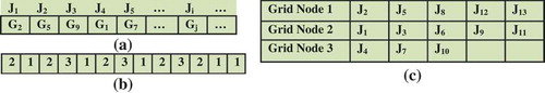
The solution is represented as an array of length equal to the number of jobs. The value corresponding to each position i in the array represent the node to which task i was allocated. The representation of the solution for the problem of scheduling 13 tasks to 3 computing nodes is illustrated in Figure 1. The first element of the array denotes the first task (n₁) in a batch, which is allocated to the computing node 2; the second element of the array denotes the second job (n₂), which is assigned to the computing node 1, and so on.

Figure 1. (a) Solution representation. (b) Solution for the problem of 13 tasks and 3 computing nodes. (c) Mapping of tasks with computing nodes for the solution given in (b).

Initial solution generation

Numerous methods have been proposed to generate the initial solution when applying meta-heuristics to the scheduling problem in the heterogeneous environment (Abraham, Liu, and Zhao 2008; Xhafa 2007; Xhafa and Duran 2008). The deterministic heuristic Min-Min algorithm has been used as a method to generate the initial solution (Algorithm A.1). This algorithm leads to more balanced schedules and generally finds smaller makespan values than other heuristics, since more tasks are expected to be assigned to the nodes that can complete them the earliest. As the Min-Min algorithm provides a good starting solution to the DAG scheduling algorithm, the VNS algorithm converges to a desired solution faster than when using the random initial solution. As GA did not produce expected good results with the Min-Min seed, GA has been experimented with random seed.

Neighborhood structures

The neighborhood structure defines the type of modifications a current solution can undergo and thus, different neighborhoods offer different ways to explore the solution space. In other words, definition of the proper neighborhood structures leads to a better exploration and exploitation of the solution space. Two attributes of the solutions are considered to define six neighborhood structures so that a larger part of the solution space can be searched and the chance of finding good solutions will be enhanced. The attributes that can be altered from one solution to another are “Random assignment of grid nodes to jobs,” and “Workload of computing nodes.” The defined neighborhood structures and corresponding moves associated with them are explained in detail below.

SwapMove

This neighborhood structure provides a set of neighbors for current solution x, based on exchanging the nodes assigned for the randomly selected three tasks.

Makespan-InsertionMove

This neighborhood assigns the Light node to the randomly selected task in the task list of Heavy node. Light and Heavy nodes are the nodes with minimum and maximum local makespan, respectively, where the local makespan of individual node gives the completion time of its latest task. Maximum local makespan is the makespan of the solution.

InsertionMove

Neighbors generated using this neighborhood structure can be constructed using the assignment of random node p₁ in P to the random task n₁ in V.

Weightedmakespan—Insertionmove

Based on this neighborhood structure, solutions are generated by assigning the random node Lr to the random task n₁ selected from the task list of the random node Hr. Lr and Hr are the nodes having local makespan value less than or equal to 0.25 and greater than or equal to 0.75 of the makespan of current solution, respectively.

BestInsertionMove

This neighborhood maps the longest task n₁ in the task list of Heavy to the node having minimum execution time for n₁.

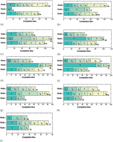
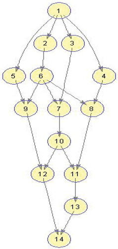
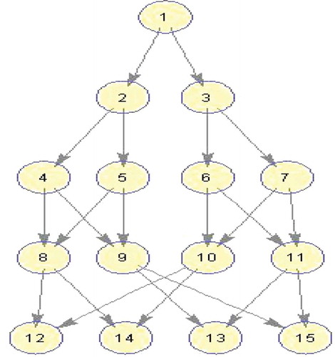
To illustrate, a small-scale DAG scheduling problem involving 3 nodes and 10 tasks is considered (Figure 2) with the computation cost matrix given in Table 1. The upward rank and the order of the tasks for execution are given in Tables 2 and 3, respectively. Consider the initial solution with makespan 126, which is represented in Figure 3(a). The Weightedmakespan—InsertionMove operator assigns the task n₇ from the task list of p₃ (considered as Hr) to the node p₂ (considered as Lr). This mapping changes the localmakespan of p₂ as 77, and maintains the makespan of the current solution as 126 [Figure 3(b)]. Then the task n₁₀ assigned for p₃ (Heavy-with localmakespan 126) is mapped with the node p₂ (Light—with localmakespan 77), according to the Makespan-InsertionMove neighborhood. Thus the fitness of the current solution becomes 117, which is illustrated in Figure 3(c). Then the BestInsertionMove neighborhood selects the longest task n₁ from p₂ (considered as Heavy) and assigns with p₃ (High-speed node of n₁). This neighborhood minimizes the fitness of current solution as 101 [Figure 3(d)]. The SwapMove operator swaps the nodes assigned for the randomly selected three jobs n₇, n₈, and n₃ (already mapped with p₂, p₁, and p_1, respectively) and changes the fitness of the solution as 98 [Figure 3(e)]. Then InsertionMove neighborhood selects the node p₃ and maps with the task n₉ (already mapped with p₁).Thus the makespan of the current solution becomes 97, which is illustrated in Figure 3(f). Again the InsertionMove neighborhood operator changes the makespan of the current solution as 93 [Figure 3(g)], by mapping the task n₅ (already mapped with p₁) with the node p₂, and then as 92 [Figure 3(h)], by mapping the task n₄ (already mapped with p₃) with the node p₂. The final solution has the makespan 73, which is the result of the application of the InsertionMove neighborhood. The task n₉ from the node p₃ is assigned to the node p₂, which is illustrated in Figure 3(i).

Figure 2. An example DAG(Topcuoglu, Hariri, and Wu 2002).

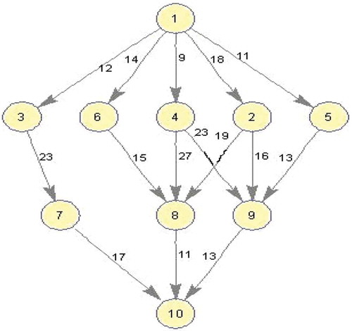
Table 1. Computation cost matrix for random DAG.

Task id	P1	P2	P3
1	14	16	9
2	13	19	18
3	11	13	19
4	13	8	17
5	12	13	10
6	13	16	9
7	7	15	11
8	5	11	14
9	18	12	20
10	21	7	16

Table 2. Upward rank of the tasks.

Task id	Upward rank
1	108.00000
2	77.00000
3	80.00000
4	80.00000
5	69.00000
6	63.33333
7	42.66667
8	35.66667
9	44.33333
10	14.66667

Table 3. Execution order of tasks.

Order of task id
1
4
3
2
5
6
9
7
8
10

Figure 3. Explanation of different neighborhood structures: (a) Initial solution, (b) Weightedmakespan–InsertionMove, (c)Makespan-InsertionMove, (d) BestInsertionMove, (e) SwapMove, (f) InsertionMove, (g) InsertionMove, (h) InsertionMove, and (i) InsertionMove.

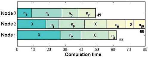
The HEFT algorithm produces the makespan of 80 (Figure 4), for example, DAG shown in Figure 2, which is greater than the makespan produced by the related work (equal to 73).

Figure 4. A schedule for the example DAG using the HEFT algorithm.

Proposed VNS grid job scheduling algorithm

VNS is a meta-heuristic that systematically exploits the idea of neighborhood change, both in descent to local minima and in escape from the valleys which contain them. The term VNS is referred to all local search-based approaches that are centered on the principle of systematically exploring more than one type of neighborhood structure during the search. VNS iterates over more than one neighborhood structures until some stopping criterion is met. The basic scheme of the VNS was proposed by Mladenovic´ and Hansen (1997). Its advanced principles for solving combinatorial optimization problems and applications were further introduced in (Hansen and Mladenovic´ 2003; Mladenovic´ and Hansen 1999, 2001) and recently in (Hansen, Mladenovic, and Urosevic 2006, 2010).

VNS uses a finite set of preselected neighborhood structures denoted as . denotes the set of solutions in the ^th neighborhood of solution.VNS employs a local search to obtain a solution called as a local minimum, such that there exists no solution with. The local search can be performed in different ways. The generic way consists of choosing an initial solution, finding a direction of descent from within a neighborhood, and moving to the minimum of within in the same direction. If there is no direction of descent, the heuristic stops; otherwise, it is iterated. After the local search, a change in the neighborhood structure is performed. Function NeighborhoodChange compares the value of a new solution with the value of the incumbent solution obtained in the neighborhood. If an improvement is obtained, is returned to its initial value and the incumbent solution is updated with the new one. Otherwise, the next neighborhood is considered.

The proposed VNS DAG scheduling algorithm is summarized in Algorithm 1. VNS uses two parameters:, which is the maximum cpu time allowed as the stopping condition, and, which is the number of neighborhood structures used. Step 4 of Algorithm 1, which is called shaking, randomly chooses a solution from the ^th neighborhood of the incumbent solution. After improving this solution via the PALSheuristic local search (Algorithm 4), a neighborhood change is employed. The fitness of the solution is evaluated based on the procedure described in the Algorithm 2.

Algorithm 1.

VNS DAG scheduling algorithm

Input:

Output:

1 repeat

2

3 repeat

4

5 /* Local search*/

6

7 until

8

9 until

Algorithm 2.

/*fitness evaluation */

Input:

Output:

1. [v, q]← size( [][])

2. ;

3. for i = 1 to v do

4. Calculate using the insertion-based scheduling policy

5. Update the

6. endfor

7.

8.

Algorithm 3.

NeighborhoodChange

 Input: ,,

 Output: ,

1 if then

2

3

4 else

5

6 endif

Algorithm 4.

PALS Heuristic

 Input: x, ,

 Output:

1 for i = 1 to do

2

3

4 Task list of Heavy

5 Select a random node p₁, where

6 list of p₁

7

8

9

10

11

12

13 for i = startheavy to endheavy do

14   for j = startres to endres

15    Swap the computing nodes assigned for JJ[i] and JJJ[j]

16    

17    if (temp < Best)

18      

19      Best ← temp

20    endif

21   endfor

22  endfor

23 if (fitnes > Best) then

24   fitnes ← Best

25   

26   break

27  endif

28 endfor

Problem aware local search (PALS)

Basic concept of this local search has been used in the literature for the DNA fragment assembly problem (Alba and Luque 2007) and the heterogeneous computing scheduling problem (Nesmachnow et al. 2012b).Working on a given schedule x, this algorithm selects a node Heavy to perform the search. The outer cycle iterates on “it” number of tasks (where it = endheavy—startheavy + 1) of the node Heavy, while the inner cycle iterates on “jt” number of tasks (where jt = endres—startres + 1) of the randomly selected node p₁, other than Heavy. For each pair (i, j), the double cycle calculates the makespan variation when swapping the nodes assigned for JJ[i] and JJJ[j], where JJ and JJJ denote the task list of the nodes Heavy and p_1, respectively. This neighborhood stores the best improvement on the makespan value for the whole schedule found in the evaluation process of it×jt. At the end of the double cycle, the best move found so far is applied. In this algorithm, startheavy and endheavy, and startres and endres are assigned with random values based on the length of array JJ and JJJ, respectively (Refer line 4 and 6 of Algorithm 4).The randomness introduced in the parameters endheavy and endres makes this local search to differ from the concept existing in the literature. The details of the neighborhood structures are given in Algorithms 5–9.

Algorithm 5.

SwapMove

 Input: x

 Output:

 1. Choose three random tasks n₁, n₂, and n₃ in V

2. Swap the computing nodes assigned for n₁, n₂, and n₃ of x

Algorithm 6.

Makespan-InsertionMove

 Input: x,

 Output:

 1. Evaluate the fitness of x

 2. Select two nodes Light and Heavy from P, where Light and Heavy are the nodes with minimum and maximum localmakespan, respectively

 3. Select a random task n₁ from the task list assigned for Heavy

 4. Assign Light to n₁

Algorithm 7.

BestInsertionMove

 Input: x,

 Output:

 1. Evaluate the fitness of x

 2. Select a longest task from the job list assigned for Heavy

 3. Select a node p₁ in P, where p₁ has minimum execution time for n₁

 4. Assign p₁ to n₁

Algorithm 8.

Weightedmakespan—InsertionMove

 Input: x,

 Output:

 1 Evaluate the fitness of x

 2 Select two random nodes Lr and Hr,

    where , and

      

 3 Select a random task n₁ from the task list assigned for Hr

 4 Assign Lr to n₁

Algorithm 9.

InsertionMove

 Input: x

 Output:

 1 Select a random task n₁ in V

 2 Select a random resource p₁ in P

 3 Assign p₁ to n₁

Computational experiments

The performance of VNS-based DAG scheduling algorithm is compared with the best existing heuristic algorithm, HEFT (Topcuoglu, Hariri, and Wu 2002), and also with the popular meta-heuristic algorithm, GA (Hou, Ansari, and Ren 1994). Since HEFT algorithm outperforms the other well-known heuristic scheduling algorithms for heterogeneous distributed computing system, HEFT algorithm has been considered for comparison. The HEFT, GA, and VNS algorithms are developed and run on the same platform in order to make a fair comparison. Two sets of graphs are used as the workload to test the performance of DAG scheduling algorithms: the randomly generated application graphs and the real-world application graphs, in which three numerical applications are considered.

The VNS-based DAG scheduling algorithm was developed using MATLAB R2010a and run on an Intel(R) Core(TM) i5 2.67 GHz with 4 GB RAM. The performance of the algorithms is evaluated based on the makespan value. For each DAG application, VNS and GA algorithms were run for 50 times, and the average of these 50 runs is reported. The evaluation of the fitness function usually requires larger computing time than the application of neighborhood operators. When the problem dimension grows, algorithm takes more time to evaluate the fitness of the solution. Hence, the maximum running time of the algorithm is not set to uniform value for all applications. The stopping condition t_max is set to 0.5*v, where v is the number of tasks of the application DAG.

Examining the performance of the algorithm parameters

This section deals with the experimentation of VNS to make two algorithm-specific decisions, namely the order of neighborhoods and the selection of neighborhoods. For taking these decisions, the proposed algorithm was run for three real-world problems, namely Gaussian Elimination algorithm with matrix size as 12, FFT algorithm with input data size of 16, and Molecular Dynamics code with communication to computation cost ratio (CCR) value of 5. In this section, 2 numbers of computing nodes are considered for the experimentation of algorithms with the real-world DAG applications. After the extensive experimentation, the combination of SwapMove, Makespan-InsertionMove, BestInsertionMove, Weightedmakespan—InsertionMove, and InsertionMove was selected for the proposed VNS. Both the parameters PALS_maxiter and are set to 5.

GA gave better results for the examined DAG applications with parameters: 10 number of population, and crossover and mutation constant as 0.5. The best solution found at the end of each generation of GA will be applied to the PALS algorithm to generate better schedule. If any improvement is achieved, then the new solution generated by the local search algorithm will replace the already found best solution. Then the next generation will be processed.

Performance results on randomly generated application graphs

The random DAGs used in this section were generated by varying a set of parameters. The random graph generator was implemented based on the concept coined by Topcuoglu, Hariri, and Wu (2002), which accepts the following parameters.

1. Size of the DAG, v: Total number of tasks in the DAG.

2. Communication to computation cost ratio, CCR: It is the ratio of the average communication cost to the average computation cost.

3. Shape of the DAG,: The height and width of the DAG are randomly chosen from a uniform distribution with the mean value of /α and, respectively, and which are rounded up to the nearest integer.

4. Computation cost heterogeneous factor β: The expected execution time of the task on the processors of the system is varied by using different values of β. The variation of execution time of task on the processor is high and low for high and low value of β, respectively.

The computation time of n_i on the computing node p_j is denoted as, which is randomly selected from

(10)

where is the average computation cost of the task n_i. is randomly chosen from the range [1,100]

Random application DAGs are generated with the following features:

Number of computing nodes q: {2, 4, 8, 16},

Number of tasks v: {20, 40, 60, 80, 100},

Value of CCR: {0.1, 0.5, 1, 2, 5},

α:{0.5,1,2},

β:{0.25,0.5,0.75,1}.

Figure 5(a) shows the performance of scheduling algorithms for various sizes of application DAGs with 2 computing nodes and CCR value of 5. VNS DAG scheduling algorithm produces less average makespan when compared with other algorithms. As the number of tasks increases, the average makespan of the application DAG is also increasing.

Figure 5. Performance results on random graphs. (a) Average Makespan with respect to DAG size. (b) Average Makespan with respect to CCR.

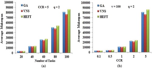
The average makespan variation of scheduling algorithms for various CCR values is shown in Figure 5(b). This experiment was conducted by considering 2 numbers of computing nodes and with 100 numbers of tasks.

Performance results on real-world applications

Three real-world applications namely Gaussian elimination (Mohammad and Kharma 2011; Topcuoglu, Hariri, and Wu 2002; Wu and Dajski 1990; Xu et al. 2013), fast Fourier transformation (Chung and Ranka 1992; Cormen, Leiserson, and Rivest 1990; Mohammad and Kharma 2011; Topcuoglu, Hariri, and Wu 2002), and a molecular dynamics code (Kim and Browne 1988; Mohammad and Kharma 2011; Topcuoglu, Hariri, and Wu 2002; Xu et al. 2013) were considered to study the performance of algorithms.

Gaussian elimination

Figure 6 shows the DAG for the Gaussian elimination algorithm for the matrix size of 5. If N is the size of the matrix, the total number of tasks in a Gaussian elimination graph is equal to . As the structure of the Gaussian elimination DAG is known, only the parameters such as CCR values and the total number of computing nodes available for scheduling were varied to generate Gaussian elimination DAGs.

Figure 6. Gaussian Elimination DAG with size 5.

The size of the matrix was varied from 5 to 20, with the increment value of 1. 0.1, 0.5,1, 2, and 5 were the CCR values used for the experimentation. The number of heterogeneous computing nodes used for the mapping of tasks was varied from 2 to 16, incrementing as a power of 2.

Figure 7(a) shows the average makespan produced by the DAG scheduling algorithm in relation to CCR. The number of processor and the size of the matrix are set to 5 and 12, respectively.

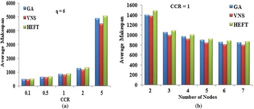
Figure 7. Performance results on Gaussian elimination DAG. (a) Average Makespan with respect to CCR. (b) Average Makespan with respect to number of computing nodes.

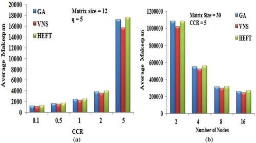
As the high value application DAGs are considered to be communication intensive, the average makespan increases with an increase in the values of CCR. From Figure 8, it is observed that the performance of VNS and GA is better when compared with HEFT. This experimentation shows that VNS is able to generate better schedules for the communication intensive applications.

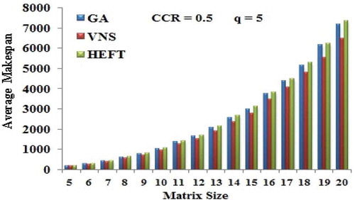
Figure 8. Average Makespan with respect to the matrix size of Gaussian elimination DAG.

Figure 7(b) gives the average makespan values of the algorithms at various number of computing nodes from 2 to 16, incrementing as a power of 2, when the size of matrix is equal to 30 and 5 as the CCR value.

The VNS algorithm is able to produce better schedules when compared with other two algorithms. As the number of computing nodes is increased for the fixed matrix size, the average makespan is found to be decreased.

Figure 8 shows the performance of the algorithm with respect to the size of the matrix, when the number of processors is equal to 5. The CCR value used for this experimentation is set to 0.5. The average makespan is found to be increased as the size of the matrix increases. This experiment was conducted with the application DAGs of various tasks ranging from 14 to 209. The performance of VNS is found to be the best of all.

Based on three kinds of experimentation, it is found that the meta-heuristic dominates the considered heuristic algorithm. Usually the meta-heuristics explore wide area of solution space to find the better mapping of tasks with computing nodes, when compared with the heuristic algorithm.

Fast Fourier transform

Figure 9 shows the DAG of FFT with four input data points. The radix 2 FFT algorithm is considered for the experimentation. Hence, if M denotes the number of input data points, then M = 2^k, where k takes integer values. Each path from the start task to any of the exit task in the FFT DAG consists of equal number of tasks. Also, in FFT DAG, the computation cost of tasks in any level is equal and the communication with all of edges between two consecutive levels is equal (Topcuoglu, Hariri, and Wu 2002).

Figure 9. Four input data point FFT DAG.

For M number of input data points of FFT DAG, total number of tasks is equal to . The input data points of FFT were varied from 2 to 64, incrementing as a power of 2. Hence, the total number of tasks ranges from 5 to 511. CCR values that were used in the experimentation are 0.1, 0.5,1, 2, and 5.

Figure 10(a) and (b) shows the average makespan of different algorithms under different number of input data points of FFT. This experimentation was conducted with the CCR value of 5 and with the total number of computing nodes of 6.

Figure 10. (a) and (b) Average Makespan with respect to the Input data points of FFT DAG.

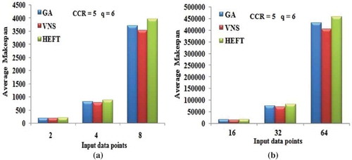
As the number of input data points increases, the average makespan is also found to be increased. The VNS DAG scheduling algorithm produces the better schedules in most of the cases.

Figure 11(a) shows the performance of algorithms for 64 input FFT DAG with respect to five different CCR values, when the number of computing node is set to be 6. VNS DAG scheduling algorithm produces better results consistently over other algorithms even for the high communication cost of DAG applications.

Figure 11. Performance results on FFT DAG. (a) Average Makespan with respect to CCR. (b) Average Makespan with respect to number of computing nodes.

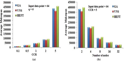
Figure 11(b) presents the average makespan values obtained by the three scheduling algorithms for 64 point FFT DAG, with respect to the various number of computing nodes, by setting the CCR value as 5.

The VNS DAG scheduling algorithm gives better schedules when compared with other scheduling algorithms. Figure 11(b) shows the decrease of makespan with the increasing number of heterogeneous computing nodes. The performance of VNS DAG scheduling algorithm is found to be good for the FFT application DAGs.

Molecular dynamics code

The performance of the scheduling algorithms was studied for the molecular dynamics code described in the reference (Kim and Browne 1988). As the structure of the considered application DAG and its number of tasks are known, the experimentation of scheduling algorithms was carried out by varying the CCR values and the number of computing nodes.

Figure 12 shows the DAG for the molecular dynamics code. Figure 13(a) shows the variation of average makespan of scheduling algorithms for the variation of CCR, by considering 6 number of computing nodes. It is obtained from the Figure 13(a) that the average makespan yielded by the VNS DAG algorithm is better, when compared with other scheduling algorithms. Also the average makespan is found to be increased, when the CCR value is increased.

Figure 12. Molecular Dynamics DAG (Topcuoglu, Hariri, and Wu 2002).

Figure 13. Performance results on Molecular Dynamics DAG. (a) Average Makespan with respect to CCR. (b) Average Makespan with respect to number of computing nodes.

Figure 13(b) shows the decrease in average makespan value with the increasing number of heterogeneous computing nodes. This experimentation was conducted with the CCR value of 1. The VNS algorithm gives the better mapping of tasks with the computing nodes almost in all cases.

Convergence trace of scheduling algorithm

In this section, experiments were conducted to show the change of makespan as VNS and GA progress during the search. The convergence trace of these algorithms was then compared. Figures 14–16 show the convergence traces for executing Gaussian elimination, FFT, and the molecular dynamics code, respectively.

Figure 14. The convergence trace for the Gaussian elimination DAG.

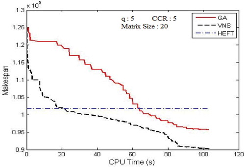
Figure 15. The convergence trace for the fast Fourier transform DAG.

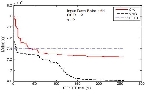
Figure 16. The convergence trace for the molecular dynamics application DAG.

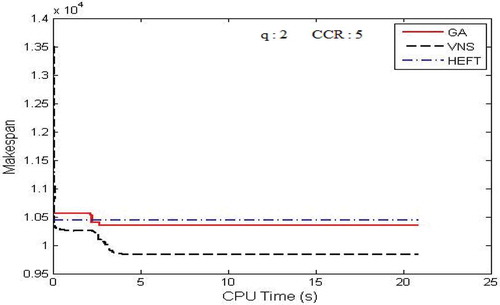
In these experiments, the stopping criteria (t_max) had been set to 0.5* v. But while considering the real-time resource management system, the stopping criteria could be set to 1 minute. It is revealed that the value of makespan decreases gradually, as both VNS and GA progress. The performance of VNS is better than the performance of GA.VNS converges faster than GA with the exploration of shorter schedule than GA. Also, GA performance was very closer to the performance of HEFT in most of the cases and did not able to compete for few DAG applications. Both VNS and GA exploit the PALS algorithm in order to escape from local minima and for the quick convergence.

Comparison with DMSCRO algorithm

Xu et al. (2013) devised and tested the DMSCRO DAG scheduling algorithm in heterogeneous computing systems. The random-generated application graphs and real-world application graphs, such as Gaussian elimination and molecular dynamics code were used to evaluate the performance of DMSCRO. The experimentation of DMSCRO reveals that DMSCRO is able to achieve the similar makespan as GA (Xu et al. 2013). The average percentage of improvement of VNS is found to be 5.51 over GA. Hence, it may be considered that the proposed VNS is able to achieve better short schedules when compared with the DMSCRO DAG scheduling algorithm.

Hybrid two-phase VNS DAG scheduling algorithm

The running time of meta-heuristic algorithms is much higher than the heuristic algorithm. Hence, the concept of hybridization of meta-heuristic with heuristic algorithm was coined by considering the scheduling time constraints imposed by the scheduler. From the previous section, it has been observed that the VNS DAG scheduling algorithm produces schedules for a variety of application DAGs, in which the initial solution was generated using Min-Min algorithm. In this section, the performance of VNS DAG scheduling algorithm was studied by considering the solution generated by the HEFT algorithm as the initial solution. Based on this concept, the HTPHVNS algorithm has been emerged. This part of the experimentation was carried out with the value of t_max considered in the previous section.

The whole part of the experimentation is repeated for all the application DAGs considered in the previous section. The percentage improvements of HTPHVNS algorithm over VNS algorithm is reported in Tables 4–13.

Table 4. Percentage improvement for random graphs with number of tasks.

Number of Tasks with CCR = 5 and q = 2
20			40			60			80			100
VNS		HTPHVNS	VNS		HTPHVNS	VNS		HTPHVNS	VNS		HTPHVNS	VNS		HTPHVNS
Over HEFT	Over GA	Over VNS	Over HEFT	Over GA	Over VNS	Over HEFT	Over GA	Over VNS	Over HEFT	Over GA	Over VNS	Over HEFT	Over GA	OverVNS
6.68	5.74	3.20	7.44	4.68	4.11	9.35	4.79	3.82	10.29	4.18	4.20	10.94	5.20	4.32

Table 5. Percentage improvement for random graphs with different CCRs.

CCR with v = 100 and q = 2
0.1			0.5			1			2			5
.VNS		HTPHVNS	VNS		HTPHVNS	VNS		HTPHVNS	VNS		HTPHVNS	VNS		HTPHVNS
Over HEFT	Over GA	Over VNS	Over HEFT	Over GA	Over VNS	Over HEFT	Over GA	Over VNS	Over HEFT	Over GA	Over VNS	Over HEFT	Over GA	Over VNS
7.66	5.10	4.29	7.97	6.88	4.17	8.80	6.36	4.03	10.76	6.24	4.6	10.94	5.20	4.72

Table 6. Percentage improvement for Gaussian elimination DAG with different CCRs.

CCR with matrix size = 12 and q = 5
0.1			0.5			1			2			5
VNS		HTPHVNS	VNS		HTPHVNS	VNS		HTPHVNS	VNS		HTPHVNS	VNS		HTPHVNS
Over HEFT	Over GA	Over VNS	Over HEFT	Over GA	Over VNS	Over HEFT	Over GA	Over VNS	Over HEFT	Over GA	Over VNS	Over HEFT	Over GA	Over VNS
9.69	4.05	4.03	10.53	7.17	3.9	11.92	7.29	4.23	11.29	6.47	4.12	10.91	8.79	4.6

Table 7. Percentage improvement for various matrix sizes of Gaussian elimination DAG.

	CCR = 0.5 and q = 5
	VNS		HTPHVNS
Matrix size	Over HEFT	Over GA	Over VNS
5	10.18	2.02	4.30
6	10.45	2.27	4.07
7	10.39	6.17	4.12
8	10.16	4.94	3.90
9	9.99	7.11	4.32
10	9.49	6.61	4.15
11	10.12	8.70	4.07
12	10.53	7.17	3.49
13	10.66	8.57	3.72
14	10.79	7.72	4.13
15	10.99	6.66	4.01
16	9.63	7.68	3.97
17	9.33	6.88	3.89
18	9.33	7.21	4.92
19	11.13	9.89	4.01
20	11.81	9.68	4.67

Table 8. Percentage improvement for Gaussian elimination DAG with the number of nodes.

Number of nodes with matrix size = 30 and CCR = 5
2			4			8			16
VNS		HTPHVNS	VNS		HTPHVNS	VNS		HTPHVNS	VNS		HTPHVNS
Over HEFT	Over GA	Over VNS	Over HEFT	Over GA	Over VNS	Over HEFT	Over GA	Over VNS	Over HEFT	Over GA	Over VNS
5.77	5.49	3.97	7.14	5.09	3.91	7.99	5.14	3.67	9.67	5.28	4.12

Table 9. Percentage improvement for FFT DAG with different CCRs.

CCR with input data point = 64 and q = 6
0.1			0.5			1			2			5
VNS		HTPHVNS	VNS		HTPHVNS	VNS		HTPHVNS	VNS		HTPHVNS	VNS		HTPHVNS
Over HEFT	Over GA	Over VNS	Over HEFT	Over GA	Over VNS	Over HEFT	Over GA	Over VNS	Over HEFT	Over GA	Over VNS	Over HEFT	Over GA	Over VNS
8.35	2.82	3.16	9.43	3.85	3.99	9.68	2.46	4.13	10.50	4.18	3.98	11.42	5.85	4.21

Table 10. Percentage improvement for FFT DAG with number of nodes.

Number of nodes with input data point = 64 and CCR = 5
2			4			8			16			32
VNS		HTPHVNS	VNS		HTPHVNS	VNS		HTPHVNS	VNS		HTPHVNS	VNS		HTPHVNS
Over HEFT	Over GA	Over VNS	Over HEFT	Over GA	Over VNS	Over HEFT	Over GA	Over VNS	Over HEFT	Over GA	Over VNS	Over HEFT	Over GA	Over VNS
9.59	5.53	4.25	7.23	4.02	4.10	15.78	7.49	3.86	12.40	5.50	3.97	14.30	6.89	3.78

Table 11. Percentage improvement for various input data points of FFT DAG.

	CCR = 0.5 and q = 5
	VNS
Input data points	Over HEFT	Over GA	Over VNS
2	7.64	2.86	3.04
4	10.13	3.88	3.80
8	10.67	4.53	4.18
16	12.37	3.36	4.22
32	12.88	4.73	3.97
64	11.42	5.85	4.13

Table 12. Percentage improvement for molecular dynamics DAG with the value of CCR.

CCR with q = 6
0.1			0.5			1			2			5
VNS		HTPHVNS	VNS		HTPHVNS	VNS		HTPHVNS	VNS		HTPHVNS	VNS		HTPHVNS
Over HEFT	Over GA	Over VNS	Over HEFT	Over GA	Over VNS	Over HEFT	Over GA	Over VNS	Over HEFT	Over GA	Over VNS	Over HEFT	Over GA	Over VNS
9.52	4.79	4.09	9.34	4.45	4.13	8.93	5.74	3.97	11.30	8.18	4.31	11.18	7.96	4.87

Table 13. Percentage improvement for molecular dynamics DAG with number of nodes.

	CCR = 1
	VNS		HTPHVNS
Number of nodes	Over HEFT	Over GA	Over VNS
2	7.06	1.39	3.01
3	7.95	4.77	4.12
4	8.19	4.99	4.23
5	8.34	6.48	3.94
6	8.93	5.74	3.79
7	8.53	5.85	3.69

From the tables, it is observed that the performance of HTPHVNS algorithm is better when compared with basic VNS algorithm.

The first phase of the HTPHVNS algorithm, HEFT generates a good quality schedule. The schedule solution generated by the HEFT algorithm is considered as the initial solution for the VNS DAG scheduling algorithm in the second phase. The VNS DAG scheduling algorithm explores into a wide area of solution phase, which in turn generates shorter schedules.

By extracting the features of HEFT algorithm, HTPHVNS algorithm is able to meet the requirement of scheduler with both strict execution time requirements and loose execution time requirements. HTPHVNS algorithm meets the requirement of strict execution time scheduler by means of allowing the second phase of algorithm to run for the time that is permitted by the scheduler in order to improve the quality of schedule generated by the first phase .On the other hand, if there is no execution time constraints imposed by the scheduler, the second phase of HTPHVNS works for the maximum allowable running time of HTPHVNS algorithm. So HTPHVNS algorithm will generate high-quality schedule. Hence, HTPHVNS DAG scheduling algorithm is flexible to the user by allowing the termination of algorithm while executing the second phase at any time of requirement.

Conclusion

Grid computing has emerged as one of the hot research areas in the field of computer networking. Scheduling, which decides how to distribute tasks to resources, is one of the most important issues. This paper deals with the meta-heuristic and heuristic-based DAG scheduling algorithms in order to minimize makespan. The performance of considered algorithms was studied for 15,000 DAGs including random DAGs and real-world application DAGs. The average percentage of improvement of VNS is found to be 5.51 over GA and 9.87 over HEFT algorithm. By considering the execution time requirements of the scheduler, HTPHVNS DAG scheduling algorithm had been proposed. Compared with VNS, HTPHVNS algorithm achieves the makespan reduction of 4.07% on average.

References

- Abraham, A., H. Liu, and M. Zhao. 2008. Particle swarm scheduling for work-flow applications in distributed computing environments. Studies in Computational Intelligence 128:327–42.
- Ahmad, I., and Y. Kwok. 1994. A new approach to scheduling parallel programs using task duplication. Proceedings Int’l Conference Parallel Processing 2:47–51.
- Alba, E., and G. Luque. 2007. A new local search algorithm for the DNA fragment assembly problem. Proceedings of 7th European Conference on Evolutionary Computation in Combinatorial Optimization, vol. 4446 of Lecture Notes in Computer Science, Berlin, Heidelberg, Springer, 1–12.
- Amini, A., T. Y. Wah, M. Saybani, and S. Yazdi. 2011. A study of density-grid based clustering algorithms on data streams. Proceedings of 8th International Conference on Fuzzy Systems and Knowledge Discovery, FSKD, Shanghai, China, 3, 1652–56.
- Audet, C., J. Brimberg, P. Hansen, and N. Mladenovi´C. 2004. Pooling problem: Alternate formulation and solution methods. Management Science 50:761–76. doi:10.1287/mnsc.1030.0207.
- Bajaj, R., and D. Agrawal. 2004. Improving scheduling of tasks in a heterogeneous environment. IEEE Transactions on Parallel and Distributed Systems 15 (2):107–18. doi:10.1109/TPDS.2004.1264795.
- Bansal, S., P. Kumar, and K. Singh. 2003. An improved duplication strategy for scheduling precedence constrained graphs in multiprocessor systems. IEEE Transactions on Parallel and Distributed Systems 14 (6):533–44. doi:10.1109/TPDS.2003.1206502.
- Behnamian, J., and M. Zandieh. 2013. Earliness and tardiness minimizing on a realistic hybrid flowshop scheduling with learning effect by advanced metaheuristic. Arabian Journal for Science and Engineering 38:1229–42. doi:10.1007/s13369-012-0347-6.
- Boyer, W. F., and H. Gs. 2005. Non-evolutionary algorithm for scheduling dependent tasks in distributed heterogeneous computing environments. Journal of Parallel and Distributed Computing 65 (9):1035–46. doi:10.1016/j.jpdc.2005.04.017.
- Brimberg, J., P. Hansen, K.-W. Lih, N. Mladenovi´C, and M. Breton. 2003. An oil pipeline design problem. Operations Research 51:228–39. doi:10.1287/opre.51.2.228.12786.
- Chen, T., B. Zhang, X. Hao, and Y. Dai. 2006. Task scheduling in grid based on particle swarm optimization. Proceedings of the 5th International Symposium on Parallel and Distributed Computing (ISPDC’06), Timisoara, Romania, 238–45.
- Chitra, P., R. Rajaram, and P. Venkatesh. 2011. Application and comparison of hybrid evolutionary multiobjective optimization algorithms for solving task scheduling problem on heterogeneous systems. Applied Soft Computing 11:2725–34. doi:10.1016/j.asoc.2010.11.003.
- Chung, Y., and S. Ranka. 1992. Applications and Performance analysis of a compile-time optimization approach for list scheduling algorithms on distributed memory multiprocessors. Proceedings of the Super Computing, Minneapolis, 512–21, November.
- Coffman, E. G. 1976. Computer and jop-shop scheduling theory. New York, NY: John Wiley & Sons Inc.
- Cormen, T. H., C. E. Leiserson, and R. L. Rivest. 1990. Introduction to algorithms. MIT Press, Cambridge.
- Correa, T. C., A. Ferreria, and P. Rebreyend. 1996. Integrating list heuristics into Genetic Algorithms for Multiprocessor Scheduling. Proceedings of the 8th IEEE Symposium on Parallel and Distributed processing (SPDP’96), New Orleans, Louisiana, October.
- Costa, M. C., F. R. Monclar, and M. Zrikem. 2005. Variable neighborhood decomposition search for the optimization of power plant cable layout. Journal of Intelligent Manufacturing 13:353–65. doi:10.1023/A:1019980525722.
- Darling, A. E., L. Carey, and W. Feng. 2003. The design, implementation and evaluation of mpi BLAST. Proceedings of the 4th LCI International Conference on Linux Clusters: The HPC Revolution 2003, San Jose, California, June.
- El-Rewin, H., and T. Lewis. 1990. Scheduling parallel program tasks onto arbitrary target machines. Journal of Parallel and Distributed Computing 9:138–53. doi:10.1016/0743-7315(90)90042-N.
- El-Rewini, H., T. G. Lewis, and H. H. Ali. 1994. Task scheduling in parallel and distributed systems. New Jersey, NJ: Prentice Hall.
- Ferrandi, F., P. Lanzi, C. Pilato, D. Sciuto, and A. Tumeon. 2010. Ant colony heuristic for mapping and scheduling tasks and commucnication on heterogeneous embedded systems. IEEE Transactions on Computer- Aided Design of Integrated Circuits and Systems 29 (6):911–24. doi:10.1109/TCAD.2010.2048354.
- Foster, I., and C. Kesselman. 2004. The Grid 2: Blueprint for a new computing infrastructure, 2nd ed. San Francisco, California, USA: Elsevier and Morgan Kaufmann.
- Freund, R. F., and H. J. Siegel. 1993. Heterogeneous processing. IEEE Computer 26 (6):13–17.
- Garey, M. R., and D. S. Johnson. 1979. Computers and intractability: A guide to the theory of NP-completeness. New York, NY: W.H. Freeman and Co.
- Hamidzadeh, B., L. Y. Kit, and D. J. Lija. 2000. Dynamic task scheduling using online optimization. IEEE Transactions Parallel Distributed Systems 11 (11):1151–63. doi:10.1109/71.888636.
- Hansen, P., and N. Mladenovic´. 2003. An introduction to variable neighborhood search. In Handbook of MetaHeuristics, Eds. F. Glover and G. A. Kochenberger, 145–84. Amsterdam, Netherlands: Kluwer [Chapter 6].
- Hansen, P., N. Mladenovi´C, and J. A. Moreno Pérez. 2008. Variable neighborhood search: Methods and applications. 4OR A Quarterly Journal of Operations Research 6:319–60. doi:10.1007/s10288-008-0089-1.
- Hansen, P., N. Mladenovic´, and J. Moreno Pérez. 2010. Developments of variable neighborhoodsearch. Annals of Operations Research 175 (1):367–407. doi:10.1007/s10479-009-0657-6.
- Hansen, P., N. Mladenovic, and D. Urosevic. 2006. Variable neighborhood search and local branching. Computers and Operations Research 33 (10):3034–45. doi:10.1016/j.cor.2005.02.033.
- He, L., S. A. Jarvis, D. P. Spooner, H. Jiang, D. N. Dillenberger, and G. R. Nudd. 2006. Allocating non-real-time and soft real-time jobs in multiclusters. IEEE Transactions on Parallel and Distributed Systems 17 (2):99–112. doi:10.1109/TPDS.2006.18.
- Hou, E., N. Ansari, and H. Ren. 1994. A genetic algorithm for multiprocessor scheduling. IEEE Transactions on Parallel and Distributed Systems 5 (2):113–20. doi:10.1109/71.265940.
- Hwang, J., Y. Chow, F. Anger, and C. Lee. 1989. Scheduling precedence graphs in systems with interprocessor communication times. SIAM Journal on Computing 18 (2):244–57. doi:10.1137/0218016.
- Ilavarasan, E., P. Thambidurai, and R. Mahilmannan. 2005. Performance effective task scheduling algorithm for heterogeneous computing system. Proceedings of the 4th International Symposium on Parallel and Distributed Computing, France, 28–38.
- Iosup, A., C. Dumitrescu, D. Epema, H. Li, and L. Wolters. 2006. How are real grids used? The analysis of four grid traces and its implications. Proceedings of the 7th IEEE/ACM International Conference on Grid Computing, Spain, 262–69.
- Kashani, M., and M. Jahanshahi. 2009. Using simulated annealing for task scheduling in distributed systems. Proceedings of the International Conference on Computational Intelligence, Modelling and Simulation (CSSim’09), Brno, Czech Republic 265–69.
- Kim, S. J., and J. C. Browne. 1988. A general approach to mapping of parallel computation upon multiprocessor architectures. Proceedings of International Conference on Parallel Processing, 2, 1–8.
- Kim, J., J. Rho, J. O. Lee, and M. C. Ko. 2005. CPOC: Effective static task scheduling for grid computing. Proceedings of the International Conference on High Performance Computing and Communications, Italy, 477–86.
- Kruatachue, B., and T. G. Lewis. 1988. Grain size determination for parallel processing. IEEE Software 5:23–32. doi:10.1109/52.1991.
- Kwok, Y. K., and I. Ahmad. 1996. Dynamic critical-path scheduling: An effective technique for allocating task graphs to multiprocessors. IEEE Transactions on Parallel and Distributed Systems 7:506–21. doi:10.1109/71.503776.
- Kwok, Y. K., and I. Ahmad. 1999. Static scheduling algorithms for allocating directed task graphs to multiprocessors. ACM Computation Survey 31:406–71. doi:10.1145/344588.344618.
- Liou, J., and M. A. Palis. 1996. An efficient clustering heuristic for: Scheduling DAGs on Multiprocessors. Proceedings of the Symposium on Parallel and Distributed Processing, Dallas, Texas, U.S.A., 152–156.
- Liu, H., L. Wang, and J. Liu. 2010. Task scheduling of computational grid based on particle swarm algorithm. Proceedings of the 3rd International Joint Conference on Computational Science and Optimization (CSO), Anhui Province, China, 2, 332–36.
- Loudni, S., P. Boizumault, and P. David. 2006. On-line resources allocation for ATM networks with rerouting. Computers and Operations Research 33:2891–917. doi:10.1016/j.cor.2005.01.016.
- Lusa, A., and C. N. Potts. 2008. A variable neighbourhood search algorithm for the constrained task allocation problem. Journal of the Operational Research Society 59:812–22. doi:10.1057/palgrave.jors.2602413.
- Marquis, J., G. Park, and B. Shirazi. 1997. DFRN: A new approach for duplication based scheduling for distributed memory multiprocessor systems. Proceedings of the International Conference on Parallel Processing, Geneva, Switzerland, 157–66.
- Meric, L., G. Pesant, and S. Pierre. 2004. Variable neighborhood search for optical routing in networks using latin routers. Annales Des Télécommunications/Annals of Telecommunications 59:261–86.
- Mladenovic´, N., and P. Hansen. 1997. Variable neighborhood search. Computers and Operations Research 24:1097–100. doi:10.1016/S0305-0548(97)00031-2.
- Mladenovic´, N., and P. Hansen. 1999. An introduction to variable neighborhood search. In MetaHeuristics: Advances and trends in local search paradigms for optimization, Eds., S. Voss, I. H. Osman, and C. Roucairol, 449–67. Boston, MA, USA: Kluwer Academic [Chapter 30].
- Mladenovic´, N., and P. Hansen. 2001. Variable neighborhood search: Principles and applications. European Journal of Operational Research 130:449–67. doi:10.1016/S0377-2217(00)00100-4.
- Moghaddam, K., F. Khodadadi, and R. Entezari –Maleki. 2012. A hybrid genetic algorithm and variable neighborhood search for task scheduling problem in grid environment. International Workshop on Information and Electronics Engineering Procedia Engineering 29: 3808–14
- Mohammad, I. D., and N. Kharma. 2008. A high performance algorithm for static task scheduling in heterogeneous distributed computing systems. Journal of Parallel and Distributed Computing 68:399–409. doi:10.1016/j.jpdc.2007.05.015.
- Mohammad, I. D., and N. Kharma. 2011. A hybrid heuristic–genetic algorithm for task scheduling in heterogeneous processor networks. Journal of Parallel and Distributed Computing 71:1518–31. doi:10.1016/j.jpdc.2011.05.005.
- Nesmachnow, S., E. Alba, and H. Cancela. 2012. Scheduling in heterogeneous computing and grid Environments using a parallel CHC evolutionary Algorithm. Computational Intelligence 28:131–55. doi:10.1111/coin.2012.28.issue-2.
- Nesmachnow, S., H. Cancela, and E. Alba. 2012. A parallel micro evolutionary algorithm for heterogeneous computing and grid scheduling. Applied Soft Computing 12:626–39. doi:10.1016/j.asoc.2011.09.022.
- Radulescu, A., and A. J. C. Van Gemund. 1999. On the complexity of list scheduling algorithms for distributed memory systems. Proceedings of the 13th International Conference on Supercomputing, Portland, Oregon, USA, 68–75, November.
- Shanmugapriya, R., S. Padmavathi, and S. Shalinie. 2009. Contention awareness in task scheduling using Tabu search. Proceedings of the IEEE International Advance Computing Conference (IACC), Andhra Pradesh, India 272–77.
- Shroff, P., D. W. Watson, N. S. Flann, and R. Freund. 1996. Genetic simulated annealing for scheduling data-dependent tasks in heterogeneous environments. Proceedings of the Heterogeneous Computing Workshop, Honolulu, HI, 98–104.
- Sih, G. C., and E. A. Lee. 1993. A compile-time scheduling heuristic for interconnection constrained heterogeneous processor architectures. IEEE Transactions Parallel Distributed Systems 4 (2):175–87. doi:10.1109/71.207593.
- Singh, H., and A. Youssef. 1996. Mapping and scheduling heterogeneous tasks graphs using genetic algorithms. Proceedings of the Heterogeneous Computing Workshop, Honolulu, HI, 86–97.
- Song, S., K. Hwang, and Y. K. Kwok. 2006. Risk resilent heuristics and genetic algorithms for security- assured grid job scheduling. IEEE Transactions on Computers 55 (6):703–19. doi:10.1109/TC.2006.89.
- Talukder Khaled Ahsan, A. K. M., M. Kirley, and R. Buyya. 2009. Multiobjective differential evolution for scheduling workflow applications on global Grids. Concurrency and Computation: Practice and Experience 21 (13):1742–56. doi:10.1002/cpe.v21:13.
- Topcuoglu, H., S. Hariri, and M. Y. Wu. 2002. Performance-effective and low-complexity task scheduling for heterogeneous computing. IEEE Transactions Parallel and Distributed Systems 13 (3):260–74. doi:10.1109/71.993206.
- Tsuchiya, T., T. Osada, and T. Kikuno. 1997. A new heuristic algorithm based on gas for multiprocessor scheduling with task duplication. Proceedings of the 3rd International Conference on Algorithms and Architectures for Parallel Processing, Melbourne, Australia, 295–308.
- Tumeo, A., C. Pilato, F. Ferrandi, D. Sciuto, and P. Lanzi. 2008. Ant colony optimization for mapping and scheduling in heterogeneous multiprocessor systems. Proceedings of the International Conference on Embedded Computer Systems: Architectures, Modeling, and Simulation (SAMOS), Greece, 142–49.
- Ullman, J. D. 1975. NP-complete scheduling problems. Journal of Computer and System Sciences 10 (3):384–93. doi:10.1016/S0022-0000(75)80008-0.
- Viswanathan, S., B. Veeravalli, and T. G. Robertazzi. 2007. Resource-aware distributed scheduling strategies for large-scale computational cluster/grid systems. IEEE Transactions on Parallel and Distributed Systems 18 (10):1450–61. doi:10.1109/TPDS.2007.1073.
- Wang, L. 1997. A genetic-algorithm-based approach for task matching and scheduling in heterogeneous computing environments. Journal of Parallel and Distributed Computing 47 (1):8–22. doi:10.1006/jpdc.1997.1392.
- Wang, C., J. Gu, Y. Wang, and T. Zhao. 2012. A Hybrid heuristic-genetic algorithm for task scheduling in Heterogeneous Multi-core system. Algorithms and Architectures for Parallel Processing, Lecture Notes in Computer Science 7439:153–70.
- Wen, Y., H. Xu, and J. Yang. 2011. A heuristic-based hybrid genetic-variable neighborhood search algorithm for task scheduling in heterogeneous multiprocessor system. Informatics Sciences 181:567–81. doi:10.1016/j.ins.2010.10.001.
- Wong, Y. W., R. Goh, S. H. Kuo, and M. Low. 2009 A Tabu search for the heterogeneous dag scheduling problem. Proceedings of the 15th International Conference on Parallel and Distributed Systems, ICPADS, Guangdong, China, 663–70.
- Wong, H. M., D. Yu, B. Veeravalli, and T. G. Robertazzi. 2003. Data-Intensive Grid Scheduling: Multiple Sources with Capacity Constraints. Proceedings of the 16th International Conference on Parallel and Distributed Computing and Systems (PDCS ’03) Marina del Rey, USA, 7–11.
- Wu, M., and D. Dajski. 1990. Hypertool: A programming aid for message passing systems. IEEE Transactions Parallel Distributed Systems 1 (3):330–43. doi:10.1109/71.80160.
- Xhafa, F. 2007. A hybrid evolutionary heuristic for job scheduling on computational grids. Studies in Computational Intelligence 75:269–311.
- Xhafa, F., and B. Duran. 2008. Parallel memetic algorithms for independent job scheduling in computational grids. Eds. C. Cotta, and J. van Hemert Recent Advances in Evolutionary Computation for Combinatorial Optimization, vol. 153 of Studies in Computational Intelligence, Springer-Verlag Berlin Heidelberg, 219–39.
- Xu, Y., K. Li, L. He, and T. K. Truong. 2013. A DAG scheduling scheme on heterogeneous computing systems using double molecular structure-based chemical reaction optimization. Journal of Parallel and Distributed Computing 73:1306–22. doi:10.1016/j.jpdc.2013.05.005.
- Yang, T., and A. Gerasoulis. 1994. DSC: Scheduling parallel tasks on an unbounded number of processors. IEEE Transactions Parallel and Distributed Systems 5 (9):951–67. doi:10.1109/71.308533.
- Zomaya, A., C. Ward, and B. Macey. 1999. Genetic scheduling for parallel processor systems: Comparative studies and performance issues. IEEE Transactions on Parallel and Distributed Systems 10:795–812. doi:10.1109/71.790598.