An SVM—ANN Hybrid Classifier for Diagnosis of Gear Fault

ABSTRACT

A hybrid classifier obtained by hybridizing Support Vector Machines (SVM) and Artificial Neural Network (ANN) classifiers is presented here for diagnosis of gear faults. The distinctive features obtained from vibration signals of a running gearbox, which was operated in normal and fault-induced conditions, were used to feed the SVM-ANN hybrid classifier. Time-domain vibration signals were divided in segments. Features such as peaks in time domain and in spectrum, central moments, and standard deviations were obtained from signal segments. Based on the experimental results, it was shown that SVM-ANN hybrid classifier can successfully identify gear condition and that the hybrid SVM-ANN classifier performs much better than standard versions of ANNs and SVM. The effectiveness of the hybrid classifier under noise was also investigated. It was shown that if vibration signals are preprocessed by Discrete Wavelet Transform (DWT), efficacy of the SVM-ANN hybrid is significantly enhanced.

Introduction

Gears are used in machines to pass on power from one shaft to another with change in its speed and torque. In plant industry, Gearboxes are perhaps the most critical machinery fitted in a power transmission system (Radzevich 2012). Due to its high cost, gearboxes are not readily kept in stock for replacement in the event of a catastrophic failure. Therefore, gearbox failure can potentially lay off the plant for months, due to long production time. The implementation of rapid and accurate condition monitoring system of a gearbox is an undeniable obligation due to the requirement of high reliability of gearbox.

Alteration in vibration signals emanating from machine indicates that the gear pair meshing condition is undergoing a change. Monitoring changes in vibration signal with the help of accelerometer mounted on the gearbox housing is an established method for gear damage assessment. The dominant source of vibration in gears is the interaction of the gear teeth. Even when there are no faults present, the dynamic forces that are generated produce both impulsive and broadband vibration. The discrete, impulsive vibration is associated with the various meshing impact processes, and the broadband vibration is associated with friction, fluid flow, and general gear system structural vibration (Norton and Karczub 2003).

Gear faults generally fall into the following two categories:

1. Localized faults—discrete gear tooth irregularities such as chipped tooth or missing tooth Gear.

2. Distributed faults—uniform wear on teeth all around the gear.

The main frequency at which gearing-induced vibrations will be generated is the gear meshing frequency, f_m. It is given by:

(1)

where N is the number of teeth, and f_s is the rotational speed of the gear shaft per second. A dominant peak at f_m can be observed in the spectrum, and due to the periodic nature of gear meshing, integer harmonics of f_m are also present in the spectrum. Increase in vibration levels at the gear meshing frequency and its associated harmonics is a typical criterion for fault detection.

The localized fault manifest in high vibration levels at the gear mesh frequency, fm, and its associated harmonics. Also, discrete faults tend to produce low level, flat, sideband spectra (at ± the shaft rotational speed and its associated harmonics) around the various gear meshing frequency harmonics.

Distributed faults such as uniform wear around a whole gear tend to produce high-level sidebands (at ± the shaft rotational speed and its associated harmonics) in narrow groups around the gear meshing frequencies.

The increases at the gear meshing frequency and its various harmonics are associated with fault or wear. However, in a typical gear train, several such gear meshing frequencies and their harmonics are present, which coupled with high broadband random noise that is always present in actual working gearbox, making detection of gear faults a tough task.

To solve this problem, techniques using both time domain and spectral methods have been developed for gear faults (Sharma and Parey 2016). Time domain methods make use of indicators that are able to capture “peakyness” of signal such as kurtosis, difference histograms, crest factor and peak level/rms value.

It is hard to recognize gear defect in simple vibration spectrum or by traditional time domain methods; hence, many new techniques have been employed by researchers for diagnosis of gear faults. These include techniques such as Artificial Neural Networks (ANN) (Bangalore and Tjernberg 2015; Dellomo 1999), Support Vector Machines (SVM) (Praveenkumar et al. 2014; Samanta 2004), and Wavelet Transform (Tse, Yang, and Tama 2004; Zhou et al. 2007; Yao et al. 2009).

To make the classification process faster and more effective, various researchers have demonstrated the efficacy of hybridizing ANN with SVM (Lee, Lee, and Lim et al. 2012; Seo, Roh, and Choi 2009) and combined Discrete Wavelet Transform (DWT) with ANN/SVM (Saravanan and Ramachandran 2010; Widodo and Yang 2008) for diagnosis of machinery faults.

In the present work, a hybrid SVM-ANN classifier for diagnosis of gear faults is presented. The hybrid classifier was fed with features obtained from time domain and frequency spectrum of vibration signal. The vibration (acceleration) signals were obtained from gearbox that was operated in normal (without fault) condition and with induced faults. These signals were treated with simple processing to extract features that were thereafter used to feed the ANN classifier.

The magnitude of the vibration may change with varying operating conditions such as operating speed, load, or location/sensitivity of sensor. In the present work, the signals were normalized to make them comparable regardless of differences in the magnitude. Normalized signals were used for better generalization and to ensure that the classification results are not influenced by changes in signals due to operating conditions. The results remain unaffected so long as the signal patterns are unchanged. The classifier was not fed with single values of features obtained from the signal; instead, the features set were obtained after dividing the signal in various segments. The effectiveness of the proposed classifier was also assessed under condition of noise. The acquired data set was added with Gaussian noise at different levels prior to extraction of features.

In the paper, acquisition of vibration signals and creation of features to feed the classifier were similar to the method used by Tyagi and Panigrahi 2017. However, the similarity lies only till data acquisition and creation of test and train vectors. In this paper, a novel hybrid classifier is presented. This classifier is obtained by intelligently combining the traditional ANN and SVM classifiers together, and it was shown that this fusion of SVM and ANN produces a hybrid classifier that is superior to SVM and ANN if used individually.

The hybrid classifier was created by replacing the output layer of a trained ANN by SVM (explained later in detail in Sub-Section titled ‘The hybrid classifier’). The effect of number of nodes in hidden layer on performance of classifier was also studied. The acquired vibration signal was preprocessed with DWT, and it was shown that preprocessing with DWT improves the performance of hybrid classifier for identification of gear condition. The framework of gear fault diagnosis proposed in the present work is shown in Figure 1.

Figure 1. Flowchart of diagnostic procedure.

Discrete wavelet transform and multiresolution analysis

Wavelet Transform has been successfully used for diagnosis of machinery faults. (Tse, Yang, and Tama 2004) demonstrated how Wavelet Transform is an effective tool for machinery fault diagnosis. DWT has in recent times been applied to gearbox fault diagnosis (Yao et al. 2009; Zhou et al. 2007). Various researchers have enhanced the effectiveness of traditional classifiers in diagnosis of machinery fault by employing DWT (Paya, Esat, and Badi 1997).

The nonstationary nature of machinery vibration signal makes Wavelet transforms most suitable to study them. Further, DWT also provides multiresolution analysis, which makes it possible to obtain good time resolution at high frequency band and good frequency resolution at low frequencies (Chui 1992). This property makes DWT most appropriate for analysis of vibration signal, which is inherently nonstationary and contains both high- and low-frequency components.

The Daubechies wavelet of order 44 (db44) has been found to be especially useful in machinery fault diagnosis applications as reported by Rafiee et al. (2009). Hence, db44 has been used here to carry out the DWT preprocessing of the signals.

Wavelet transform is a mathematical function that is used to divide continuous time signals or functions into different scales (frequency components), and thereafter analyze each section with resolution matched to its scale. Let x(t) be a discrete signal. The Continuous Wavelet Transform for this discrete time signal can be defined as

(2)

where is the conjugate of , which is the shifted and scaled form of the transforming function, named as “mother wavelet,” which is defined as

(3)

The transformed signal is a function of s and τ, which are the scale and translation parameters, respectively. The DWT obtained by discretization of is given by:

(4)

An algorithm to implement the above scheme was proposed by (Mallat 1989). Figure 2 illustrates the wavelet decomposition transformation algorithm as a flow diagram. DWT is carried out by sequential decomposition of signal x(t) as shown in Figure 2. At each level, the signal x(t) is convolved with the high-pass filter H and the low-pass filter L, producing two decomposed vectors D and A, respectively. The vectors D and A are thereafter downsampled by half to obtain cD and cA called detail and approximate coefficients, respectively. Downsampling is performed to ensure that the total numbers of coefficients produced in all the decomposed constituents are equal to number of samples in the input discrete signal x(t). The Multiresolution Analysis is achieved by repeating the decomposition process with approximate coefficients Ca at each level to obtain DWT coefficients at next level. The decomposition is performed till the desired resolution has been attained.

Figure 2. Wavelet transform decomposition at different levels.

Artificial neural networks (ANNs)

ANNs are defined as a highly connected array of elementary processors called neurons. ANN takes inspiration from biological learning process of human brain (Jain et al. 1996). ANNs have been widely used in recent years for practical applications such as pattern recognition, classification, function approximation, etc. (Rabuñal 2005). ANNs have also been used successfully for machinery fault detection (Paya, Esat, and Badi 1997; Tyagi and Panigrahi 2017), and recently, researchers have employed ANN for gearbox fault diagnosis (Bangalore and Tjernberg 2015; Dellomo 1999; Saravanan and Ramachandran 2010).

A typical ANN consists of one input layer, one output layer, and one or more hidden layers. Figure 3 schematically illustrates the structure of neuron. There are several neurons in each layer, and neurons in layers are connected to the neurons of adjacent layer with different connection weights. A neuron represents each node in the network shown in Figure 3. The neurons of input layer are fed with input feature vectors. Each neuron of hidden and output layers receives signals from the neurons of the previous layer multiplied by weights of the interconnection between neurons. The neuron thereafter produces output by passing the summed signal through a transfer function.

Figure 3. Artificial neural network.

Multilayer neural networks are traditionally trained by the supervised learning methods. In supervised learning model, network is provided with set of input vector and the targeted output that is desired from the network. Let for example the inputs and desired target to a neural network are:

where p_Q is an input to network and t_Q is its corresponding target (Park et al. 1991).

The network is trained iteratively. In each iteration, Mean Square Error (MSE) between target and network output is calculated. The MSE at the kth iteration is given by:

(5)

where F(x) is MSE function, t_k and a_k are the targets and output vectors at the kth iteration.

The training of network is achieved by adjusting the weights and biases so that the MSE function F(x) is minimized. Back Propagation (BP) using Levenberg-Marquardt algorithm is commonly employed to train ANN (Park et al. 1991). BP is a gradient descent method that uses the calculated MSE at each layer to adjust the value of the interconnecting weights to the neuron to minimize MSE. This process of layer-wise weight adjustment is repeated until the minimum of the error function is achieved or the MSE has reached to such a low value, which would be able to classify the input vectors correctly. The weights at mth layer in k + 1th iteration are estimated by:

(6)

Being a gradient descent process, BP is a fast and efficient algorithm that achieves convergence very quickly. However, BP like any other gradient search technique gives inconsistent and unpredictable performance when applied to complex nonlinear optimization problems such as ANNs (Curry and Morgan 1997). Due to the intricate nature of training ANNs, the error surfaces are very complex. Since the nature of BP is to converge locally, the solutions are highly dependent upon the initial random draw of weights, due to which BP algorithm is likely to get trapped in a local solution that may or may not be the global solution. This local convergence and inability to come out of local minima could present serious problems when using ANNs for practical applications.

Classification by SVM

Traditional classifiers such as ANNs are quite good classifiers, but they require large number of training sets to train for proper behavior. This may not be feasible in most real applications. SVMs are also a supervised learning model, but they work quite well in cases where only small training sets are available. SVM can be used to classify effectively using small data sets (Foody and Mathur 2006). SVMs do not suffer from the Curse of Dimensionality as it is able to manage sparse data in high-dimension data sets (Bengio et al. 2005). Hence, SVMs have better generalization than ANNs and solution provided by SVM is nearer to global solution, and it is significantly better then ANN. SVMs are not fraught with the danger of getting entrapped in local minima (Bianchini, Frasconi, and Gori 1995). In last few years, SVMs have found application in many real-world applications, such as (Shih, Chuang, and Wang 2008) utilized Support vector machines for recognition of Facial Expression and Widodo and Yang (2008) combined DWT with SVM for fault diagnosis of induction motor.

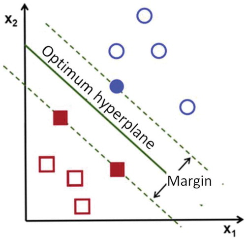
The basic idea of SVM is that it creates the optimal separation plane under linearly separable condition. The basic principle is demonstrated in Figure 4 (Vapnik and Vapnik 1998), which illustrates the classification of data set containing two different classes of data, class I (circles) and class II (squares). The SVM attempts to place an optimum hyper plane (linear boundary) between the two classes and orients it in such way that the margin (the distance between boundary and the nearest point of each class) is maximized. The nearest data points to the separating boundary are used to define the margin and are known as support vectors.

Figure 4. Classification of data by SVM.

Assume that in a given training sample set, where for each input vector , there is a desired value belonging to class defined by }. Here, yi is either +1 or −1, indicating the class to which the point xi belongs. The xi is a d-dimensional real valued vector.

SVM creates the classification function of the form:

(7)

where represents the data in feature space, and b are the coefficients. These are estimated by minimizing the following risk function:

(8)

where is the loss function that measures the approximate errors between expected output y_i and the calculated output f(x_i), and C is a regularization constant. determines the trade-off between the training error and the generalization performance. The second term in Equation (8) is used as a measure of flatness of the function. If we introduce relaxation factor ξ, ξ * it transforms Equation (8) to the following constrained function:

Finally, by introducing Lagrange multipliers and employing the optimal constraints, Equation (7) is denoted in the explicit form as

(9)

In above Eq. (10), α_i* and α_i are the Lagrange multipliers and they satisfy the equalities α_i* x α_i = 0, α_i* ≥ 0 and α_i ≥ 0. Where i being the integer valuves between 1 to N. The Lagrange multipliers α_i* and α_i are obtained by minimizing the twin Eq. (3) achieve following form:

Although nonlinear function Φ is usually unknown, all computations related to Φ could be reduced to the form Φ(x)^T. Φ(y), which can be replaced with a function known as kernel function K(x,y) = Φ(x). Φ(y). The advantage of using the kernel function is that one can deal with feature spaces of any dimension without having to compute the map explicitly. Any function that satisfies Mercer’s condition can be used as the kernel function. Four most common kernel function types of SVMs are Linear, Sigmoid, Radial Basis Function (RBF), and Polynomial Kernel. They are given as follows:

Experimental setup

The setup that was used to carry out experiments is shown in Figure 5. The setup was similar to the one used by (Tyagi and Panigrahi 2017). The experimental setup comprised a variable speed AC motor driving a gearbox shaft through flexible couplers. The gearbox consists of a 2-stage parallel shaft gearbox with four spur gears having 32, 80, 48, and 64 teeth. A magnetic break driven by belt was used to create torsional load on the system.

Figure 5. Experimental setup.

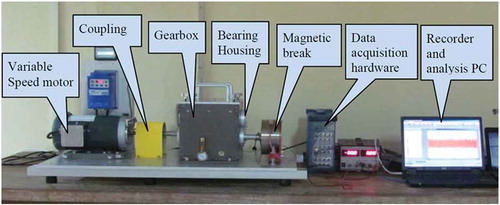
In the present work, the gear with 32 teeth was analyzed. It was mounted on load end side of the shaft to enable easy replacement. Vibration signals in form of acceleration were acquired by the accelerometer that was mounted with the help of stud on the housing of bearings that supported defective gear shaft. Three different gear faults such as missing tooth, chipped tooth, and surface wear were artificially created. Four vibration signals (acceleration) were collected for different conditions of gearbox such as gear in good condition and gearbox with defective gear having missing tooth, chipped tooth, and surface wear defects, respectively. During data recording, the load on the gearbox was set to 50%, shaft was rotated at 20 Hz speed, and the vibration signals were collected for the duration of 2 seconds each, at a sampling rate of 51.2 KSa/s; thus, each acquired signal had 102,400 samples. The following four different vibration signals were collected:

(i) gear in normal condition;

(ii) gear with missing tooth fault (MTF);

(iii) gear with chipped tooth fault (CTF);

(iv) gear with surface wear fault (SWF).

Feature extraction and training/test vectors creation

Feature extraction

The magnitude of the vibration data may vary with different kinds of faults under varying operating conditions. Making the signals comparable regardless of differences in the magnitude is achieved by normalizing by standardization. The signal is normalized by using its mean and standard deviation as per Equation (8):

(10)

where S_i denotes samples, μ is mean, and σ is standard deviation of signal. Each one of the vibration signals (i) to (iv) had 102,400 samples, which were thereafter divided in 40 nonoverlapping bins of 2560 normalized samples (y_i). Simple statistical and spectral features were extracted from these 40 bins in the similar fashion as reported by Tyagi and Panigrahi 2017. Apart from ten statistical features that were used by Tyagi and Panigrahi 2017, two additional features i.e. amplitude of both side bands to the highest peak in spectrum were also extracted in the present research. Details of twelve features extracted are as follows:

Features 1–5—Amplitude of five highest peaks of the bin.

Feature 6—Amplitude of highest peak in spectrum.

Features 7 and 8—Amplitude of side bands to the highest peak in spectrum.

Feature 9—Standard deviation σ of the bin.

Feature 10—Skewness γ₃ (third central moment) of the bin.

Feature 11—Kurtosis γ₄ (fourth central moment) of the bin.

Feature 12—Sixth central moment γ₆ of the bin.

Twelve features extracted from the acquired vibration signals of defective gears and gears in good condition showed good numerical dissimilarity with each other and therefore justify their selection. These features were used for training the SVM-ANN hybrid classifier for diagnosis of the gear condition.

Creation of training and test vectors

As explained in sub-section titled ‘Feature Extraction’ above, four signals were divided into 40 bins each. These 40 bins were divided into 24 training bins and 16 test bins. The classifier was exposed only to the training bins during training of classifier. 16 test bins that were not exposed to classifier during training were used to test the performance of the trained classifier. The training feature vectors were created by extracting features from bins of defective gears and bins of normal gear and placed them alternatively. Therefore, three sets of 48 training feature vectors denoted as MTF, CTF, and SWF were created for gear with missing tooth fault, chipped tooth fault, and surface wear fault, respectively. In a similar manner, three sets of 32 test vectors were also formed. Since 12 features were used, a training matrix of size 12 × 144 and test matrix of 12 × 96 sizes was created.

Preprocessing and addition of noise

The raw vibration signals were added with normally distributed white noise of different magnitudes to create noisy data set. Apart from creation of noisy signals, a preprocessed signal was also created by preprocessing the raw signal with Daubechies wavelet of order 44 (db44). The signal was decomposed till 1st level to obtain D1 (the high frequency detail signals at level 1). Features were extracted, and test and train vectors were created as per procedure explained in previous two sub-sections for the noisy signal and the preprocessed signal as well. Details of eight signals that were created in this step are as given below:

(a) raw signal;

(b) preprocessed with DWT at level 1 (D1);

(c) 2% added noise (peak to peak);

(d) 4% added noise (peak to peak);

(e) 6% added noise (peak to peak);

(f) 8% added noise (peak to peak);

(g) 10% added noise (peak to peak);

(h) 20% added noise (peak to peak).

Designing the SVM-ANN hybrid classifiers for gear condition diagnosis

The SVM-ANN hybrid classifier presented in this paper processes the input feature vectors in two stages first by ANN, thereafter by the SVM. The creation of hybrid ANN-SVM classifier involves the following:

(a) Training a pure feed foreword ANN classifier in traditional way using back propagation (BP) algorithm (Park et al. 1991).

(b) Replacement of output layer of ANN by SVM.

(c) Training of SVM by output of the truncated ANN.

The primary aim of replacing the output layer with SVM is to reduce the tendency of ANN to converge to a local minima resulting in under-fitting and at the same time avoid tendency of SVM to over-fit. Framework of the SVM-ANN hybrid training and diagnosis of gear fault is shown in Figure 1.

ANN classifier

A simple ANN with one hidden layer was created. The number of neurons in input layer was 12 (equal to length of feature vectors). Nodes in hidden layer were varied from 1 to 15. The output layer was made with only one neuron, and in training stage, targets were set to {1} for good gear and {0} for defective gear. The network was trained by BP of errors. Details of training and stopping criteria are given as follows:

Table

Training	Using Back propagation with Levenberg-Marquardt algorithm.
	Learning rate = 10^–7
Stopping criteria	Number of iteration <15,000,
	Gradient > 10^–6
	Mean Square error ≤ 10^–8

Post training, the ANN was simulated with test and training vectors. The criterion that was used to classify the output of the ANN classifier during simulation is:

• Input vector from defective gear was considered to be correctly classified only if the output from output layer lies within [0 ± 0.5].

• Input vector from gear in good condition was considered to be correctly classified if output lies within [1 ± 0.5] range.

Fifteen networks were created by varying the nodes of the hidden layer from 1 to 15. The input and output layers were kept unchanged. These networks were trained with training vectors created from raw signal, preprocessed signal, and noise added signals as explained in section titled ‘Feature extraction and training/test vectors creation’.

Success achieved by ANN classifier

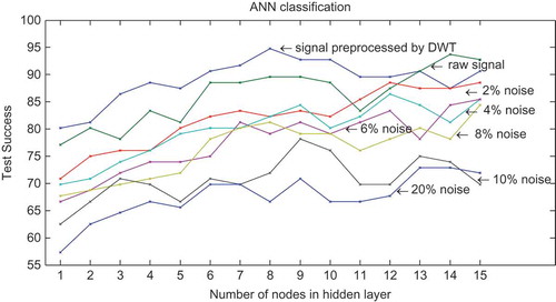
The results of successes obtained by feeding these fifteen trained ANNs by test vectors created from raw signal, preprocessed signal, and noise-added signals are presented in Figure 6. The test success obtained by raw signal (i.e. unprocessed and without addition of noise) is fairly good. 77% of 96 test vectors were correctly classified when the ANN with only one node in hidden layer was used as classifier. The test success increased as the nodes in hidden layer were increased. Network achieved 92.7% success in case of ANN with 15 nodes in hidden layer. It can be seen from Figure 6 that the test success of ANN reduced significantly with increase in magnitude of the added noise. In case of signal with 20% added noise, the test success varied from 57% (in case of 1 node in hidden layer) to 72% (15 nodes in hidden layer). The preprocessing with DWT has improved the test performance of the network. It can be seen that the success achieved with DWT preprocessed signal was higher than that with raw signal. Figure 6 shows that when nodes in hidden layers are varied from 1 to 15, the DWT preprocessed signal achieved better success than raw signal in 13 of 15 cases.

Figure 6. Test success by ANN classifier.

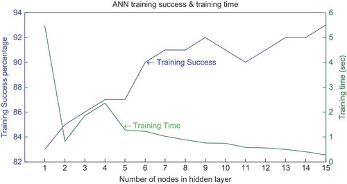
Figure 7 presents the success achieved by the classifier when it was input with the training vectors. Figure 7 presents the average success by adding successes achieved by all eight signals as mentioned in sub-section titled Pre-processing and addition of noise. It can be seen that the ANN classifier was able to achieve poor success percentages when the nodes in hidden layer were low (1–5). As nodes in hidden layer were increased, the training success improved. Low test success in cases of hidden layer nodes less than 5 coupled with low training success indicative of under-fitting.

Figure 7. Training success and training time by ANN classifier.

Training time of ANN classifier

Figure 7 also presents the average time taken by network to train when node in hidden layer was varied from 1 to 15. The training time graph is obtained by taking average of the time taken by all eight signals (i.e. raw, preprocessed and added noise). It is evident that the network took long time to train (5.5 seconds for ANN with only one node in hidden layer). As the number of nodes in hidden layer increased, the training time reduced significantly (0.3 second for ANN with 15 nodes in hidden layer).

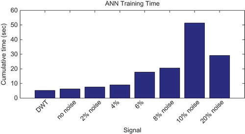
Figure 8 presents the cumulative training time signal wise. The training time data presented in Figure 8 are obtained by summing the time taken by all 15 networks. It can be seen that the training time increases as magnitude of added noise is increased. It can also be seen that preprocessing with DWT reduces the training time for ANN. The cumulative training time for DWT preprocessed signal was 5.1 seconds in comparison to 6.2 seconds for unprocessed raw signal.

Figure 8. Effect of signal type on training time.

SVM classifier

Pure SVM classifier (i.e. without hybridization) was also used to diagnose the gear condition to check its effectiveness in diagnosis of gear fault. The training and test vectors that were used for ANN classifier in previous section were also used as training and test vectors for SVM classifier. The results presented in this section are for case of signal with added 20% noise (refer sub-section titled Pre-processing and addition of noise). SVMs with Linear, Sigmoid, RBF, and Polynomial kernels were tried. It was found that SVMs using Linear and Sigmoid kernels are not suitable for gear fault diagnosis application as SVMs using Linear and Sigmoid kernels could not achieve convergence in many cases. The training process was perforce stopped after reaching maximum number of iterations (200,000). However, the Polynomial kernels and RBF kernels achieved convergence in all 15 cases.

Polynomial kernel

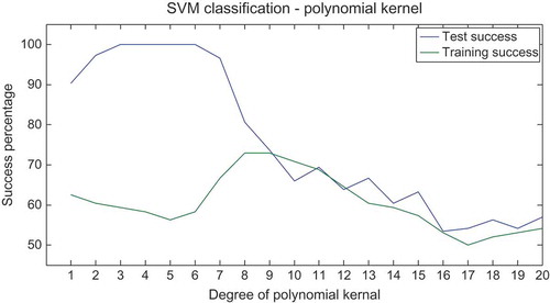
Success percentage obtained by SVM using polynomial kernel is shown in Figure 9. The degree of polynomial kernel was varied from 1 to 20 to choose the degree of polynomial that would give the most optimal solution. The inspection of results that are presented in Figure 9 reveals that SVM was under-fitting when degree of polynomial was between 16 and 20, as both train and test successes were poor (50%—60%). Over-fitting was observed for degree of polynomial between 1 and 6; as the train successes were more than 90% but corresponding test success were poor (< 65%). Maximum test success of 73% was obtained when polynomial kernel of 8 degree was used.

Figure 9. SVM with polynomial kernel train and test success.

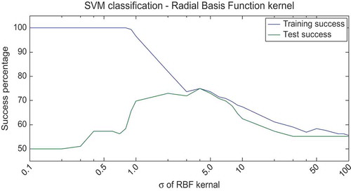
RBF kernel

Result of SVM classification obtained by using RBF kernel is shown in Figure 10. To choose the sigma that would give the most optimal solution, the sigma of RBF kernel was varied from 0.1 to 100. The inspection of results that are presented in Figure 10 reveals that test and train success percentages achieved for sigma values more than 30 were very low (~ 55%). This indicates that SVM was under-fitting for sigma values more than 30. Over-fitting was observed for sigma values from 0.1 to 0.9 as the training success was 100% in these cases but the corresponding test success achieved was very poor (50–58%). As the sigma value was reduced below 30, both test and train successes increased. Maximum test success of 75% was achieved when sigma was equal to 4. The test success started to decrease as sigma value was reduced less than 4.

Figure 10. Test and train success by SVM with RBF kernel.

Performance of SVM to correctly classify test vectors with RBF kernel was better than that with polynomial kernel; hence, RBF kernel with sigma value 4 was selected to build the hybrid classifier. The training success, training time, and test success achieved by SVM classifier using RBF kernel with sigma equal to 4 are tabulated in Table 1.

Table 1. Success and training time of SVM with RBF (σ = 4.0).

Signal	Test success	Training success	Training time (second)
Raw signal	85	100	0.0948
Preprocessed with DWT	86	100	0.0543
2% added noise	83	95	0.0454
4% added noise	80	87	0.0432
6% added noise	80	91	0.0408
8% added noise	78	84	0.0427
10% added noise	74	80	0.0403
20% added noise	75	75	0.017

The hybrid classifier

The SVM-ANN hybrid classifier was created by adding together ANN and SVM classifiers. The ANN classifier was first trained with features extracted from vibration signal as explained in sub-section titled ANN Classifier. The output of hidden layer of the ANN was used to train the SVM keeping same targets. On completion of SVM training, we get the trained hybrid SVM-ANN classifier, which is schematically depicted in Figure 11.

Figure 11. SVM–ANN hybrid classifier.

Classification success of hybrid classifier

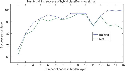
Post training of the hybrid classifier, the hybrid classifier was fed with test and training vectors to check its performance. Figure 12 presents the performance of hybrid classifier with respect to number of nodes in hidden layer of ANN. In Figure 12, the performance of hybrid classifier when it was input with features obtained from raw signal is presented. Poor success percentage for test as well as training vectors when the nodes in hidden layer were less than 3 are indicative of under-fitting. Both test and training successes improved as number of nodes in hidden layer were increased till 12. For number of nodes from 13 to 15, over-fitting can be observed as very high training success (~ 100%) corresponded to low test success. Under-fitting and over-fitting problem can be avoided with careful selection of nodes in hidden layer. Best test success (96.8%) was achieved by the hybrid classifier when nine nodes were used in the hidden layer of ANN.

Figure 12. Performance of hybrid classifier with raw signal.

Comparison of hybrid classifier with SVM

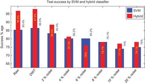
Figure 13 presents the comparison of test successes achieved by the hybrid classifier and the SVM classifier. In Figure 13, performance of hybrid classifiers with nine nodes in the hidden layer of ANN is compared with that of SVM classifier that used RBF kernel with sigma equal to 4. Performances of hybrid classifiers and SVM classifier on raw signal, signal preprocessed with DWT and noise added signals are presented in Figure 13. It was found that the hybrid classifier has performed significantly better than the SVM classifier, as for six of eight signals, hybrid classifier success was more than that of SVM. For raw and DWT preprocessed signal, the performance of hybrid classifier was about 11% higher than that achieved by SVM classifier.

Figure 13. Comparative performance of SVM and hybrid classifier.

Comparison of hybrid classifier with ANN

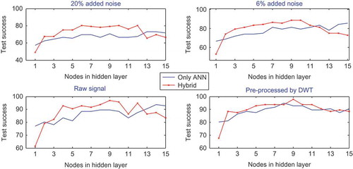
Figure 14 presents the comparison of test successes achieved by the hybrid classifier and the ANN for fifteen cases of varying number of nodes in hidden layer. Figure 14 presents the comparative plots for four different signals i.e. for raw signal, DWT preprocessed signal, 6% added noise, and 20% added noise. It is evident from these plots that performance of hybrid classifier is much superior than ANN classifier. In eleven cases of 15, the test performance of hybrid classifier was better than that of ANN. The improved performance can be seen for all four different types of signals that are presented in Figure 14. Another noteworthy aspect of the result presented in Figure 14 is that the hybrid classifier is able to diagnose the gear condition with good accuracy even in the presence of noise.

Figure 14. Comparative plots of test success by hybrid classifier versus ANN.

The average time taken to train ANN classifiers was 1.23 second, and the average time taken by SVM to train was 0.047 second, which is insignificant. Thus, it can be deduced that the additional training of SVM post training, the ANN has not caused any significant increase in the overall training time.

Conclusion

An ingenious SVM-ANN hybrid classifier to identify gear condition is presented here. The hybrid classifier was created by replacing the output layer of ANN by SVM classifier. Simple features created from magnitude of highest peaks in time domain, peaks in frequency spectrum, and statistical central moments of time-domain vibration signal. It was shown that hybrid classifier is able to correctly diagnose gearbox condition with high accuracy when trained with these simple features.

Vibration data from gearbox in good conditions and with defects induced were obtained. Additional signals were created by preprocessing the acquired vibration signal with DWT and by adding noise. Features were extracted from the vibration, and the created signals were fed to train hybrid classifier. It was shown that two-stage training presented here do not significantly increase training time. It was also shown that the hybrid classifier is able to correctly classify the gear condition even in the event of noise.

The performance of the hybrid classifier was found to be significantly better than that of pure SVM and ANN classifiers. It was also shown that by carefully choosing the number of nodes in hidden layer, the propensity of ANN to under-fit and the tendency of SVM to over-fit the input vectors can be avoided.

References

- Bangalore, P., and L. B. Tjernberg. 2015. An artificial neural network approach for early fault detection of gearbox bearings. IEEE Transactions on Smart Grid 6 (2):980–87. doi:10.1109/TSG.2014.2386305.
- Bengio, Y., O. Delalleau, and N. Le Roux. 2005. The curse of dimensionality for local kernel machines. Technical Reports:1258. http://www-labs.iro.umontreal.ca/~lisa/pointeurs/tr1258.pdf
- Bianchini, M., P. Frasconi, and M. Gori. 1995. Learning without local minima in radial basis function networks. IEEE Transactions on Neural Networks 6 (3):749–56. doi:10.1109/72.377979.
- Chui, C. K. 1992. Wavelets: A tutorial in theory and applications. In Wavelet analysis and its applications, ed. C. K. Chui, vol. 1. San Diego, CA: Academic Press.
- Curry, B., and P. Morgan. 1997. Neural networks: A need for caution. OMEGA International Journal of Management Sciences 25:123–33. doi:10.1016/S0305-0483(96)00052-7.
- Dellomo, M. R. 1999. Helicopter gearbox fault detection: A neural network based approach. Journal of Vibration and Acoustics 121 (3):265–72. doi:10.1115/1.2893975.
- Foody, G. M., and A. Mathur. 2006. The use of small training sets containing mixed pixels for accurate hard image classification: Training on mixed spectral responses for classification by a SVM. Remote Sensing of Environment 103 (2):179–89. doi:10.1016/j.rse.2006.04.001.
- Jain, A. K., J. Mao, and K. M. Mohiuddin. 1996. Artificial neural networks: A tutorial. IEEE Computer 29 (3):31–44. doi:10.1109/2.485891.
- Lee, S. M., S. H. Lee, J. Lim, et al. 2012. Defect diagnostics of power plant gas turbine using hybrid SVM-ANN method. Proceedings of the ASME Gas Turbine India Conference (GTINDIA’12), Mumbai, Maharashtra, India. 1–8.
- Mallat, S. G. 1989. A theory for multiresolution signal decomposition: The wavelet representation. IEEE Transactions on Pattern Analysis and Machine Intelligence 11 (7):674–93. doi:10.1109/34.192463.
- Norton, M. P., and D. G. Karczub. 2003. Fundamentals of noise and vibration analysis for engineers. Cambridge University Press.
- Park, D. C., M. A. El-Sharkawi, R. J. Marks, L. E. Atlas, and M. J. Damborg. 1991. Electric load forecasting using an artificial neural network. IEEE Transactions on Power Systems 6 (2):442–49. doi:10.1109/59.76685.
- Paya, B. A., I. I. Esat, and M. N. Badi. 1997. Artificial neural network based fault diagnostics of rotating machinery using wavelet transforms as a preprocessor. Mechanical Systems and Signal Processing 11 (5):751–65. doi:10.1006/mssp.1997.0090.
- Praveenkumar, T., M. Saimurugan, P. Krishnakumar, and K. I. Ramachandran. 2014. Fault diagnosis of automobile gearbox based on machine learning techniques. Procedia Engineering 97:2092–98. doi:10.1016/j.proeng.2014.12.452.
- Rabuñal, J. R., ed. 2005. Artificial neural networks in real-life applications. Hershey, New York: Information Science Reference (an imprint of IGI Global), November 30.
- Radzevich, S. P. 2012. Dudley’s handbook of practical gear design and manufacture. CRC Press, Taylor & Francis Group, Boca Raton, Florida.
- Rafiee, J., M. A. Rafiee, N. Prause, and P. W. Tse. 2009. Application of Daubechies 44 in machine fault diagnostics. Proceedings of the 2nd International Conference on Computer, Control and Communication, Karachi, IEEE, 1–6. doi: 10.1109/IC4.2009.4909247.
- Samanta, B. 2004. Gear fault detection using artificial neural networks and support vector machines with genetic algorithms. Mechanical Systems and Signal Processing 18 (3):625–44. doi:10.1016/S0888-3270(03)00020-7.
- Saravanan, N., and K. I. Ramachandran. 2010. Incipient gear box fault diagnosis using discrete wavelet transform (DWT) for feature extraction and classification using artificial neural network (ANN). Expert Systems with Applications 37 (6):4168–81. doi:10.1016/j.eswa.2009.11.006.
- Seo, D. H., T. S. Roh, and D. W. Choi. 2009. Defect diagnostics of gas turbine engine using hybrid SVM-ANN with module system in off-design condition. Journal of Mechanical Science and Technology 23:677–85. doi:10.1007/s12206-008-1120-3.
- Sharma, V., and A. Parey. 2016. A review of gear fault diagnosis using various condition indicators. Procedia Engineering 144:253–63. doi:10.1016/j.proeng.2016.05.131.
- Shih, F. Y., C. F. Chuang, and P. S. Wang. 2008. Performance comparisons of facial expression recognition in JAFFE database. International Journal of Pattern Recognition and Artificial Intelligence 22 (3):445–59. doi:10.1142/S0218001408006284.
- Tse, P. W., W. Yang, and H. Y. Tama. 2004. Machine fault diagnosis through an effective exact wavelet analysis. Journal of Sound and Vibration 277:1005–24. doi:10.1016/j.jsv.2003.09.031.
- Tyagi, S., and S. K. Panigrahi. 2017. A DWT and SVM based method for rolling element bearing fault diagnosis and its comparison with Artificial Neural Networks. Journal of Applied and Computational Mechanics. Apr 6;3(1):80–91.
- Vapnik, V. N., and V. Vapnik. 1998. Statistical learning theory. New York, USA: Wiley.
- Widodo, A., and B. S. Yang. 2008. Wavelet support vector machine for induction machine fault diagnosis based on transient current signal. Expert Systems with Applications 35 (1):307–16. doi:10.1016/j.eswa.2007.06.018.
- Yao, X., C. Guo, M. Zhong, Y. Li, G. Shan, and Y. Zhang. 2009. Wind turbine gearbox fault diagnosis using adaptive morlet wavelet spectrum. Proceedings of the Second International Conference on Intelligent Computation Technology and Automation (ICICTA’09), October 10, vol. 2, 580–83. IEEE. doi:10.1109/ICICTA.2009.375
- Zhou, G. H., C. C. Zuo, J. Z. Wang, and S. X. Liu. 2007. Gearbox fault diagnosis based on wavelet-AR model. Proceedings of the International Conference on Machine Learning and Cybernetics, vol. 2, 1061–65. IEEE, August 19. doi:10.1109/ICMLC.2007.4370300