A Comparative Analysis of SVM and IDNN for Identifying Penguin Activities

ABSTRACT

Where, when and how much animals eat provide valuable insights into their ecology. In this paper, we present a comparative analysis between Support Vector Machine (SVM) and Input Delay Neural Network (IDNN) models to identify prey capture events from penguin accelerometry data. A pre-classified dataset of 3D time-series data from back-mounted accelerometers was used. We trained both the models to classify the penguins’ behavior at intervals as either ‘prey handling’ or ‘swimming’. The aim was to determine whether IDNN could achieve the same level of classification accuracy as SVM, but with reduced memory demands. This would enable the IDNN model to be embedded on the accelerometer micro-system itself, and hence reduce the magnitude of the output data to be uploaded. Based on the classification results, this paper provides an analysis of the two models from both an accuracy and applicability point of view. The experimental results show that both models achieve an equivalent accuracy of approx. 85% using the featured data, with a memory demand of 0.5 kB for IDNN and 0.7 Mb for SVM. The raw accelerometer data let us improve the generalizability of the models with a slightly lower accuracy to around 80%. This indicates that the IDNN model can embed on the accelerometer itself, reducing problems associated with raw time-series data retrieval and loss.

Introduction

Understanding when, where and how much food animals eat under different conditions provides valuable insight into their ecology. This is particularly important for marine animals such as seabirds, which must find food in ocean environments where prey availability is dynamic (Carroll et al. 2016) and is likely to be affected by multiple pressures including climate change (Yasuda 1999) and overfishing (Cury 2011). However, directly observing marine animals foraging in the wild is challenging, as they may travel large distances from land (Burton 1999) and/or consume prey underwater (Sutton, 2015). Hence, remote activity monitoring using telemetry technology is often the only way to identify the behavior of animals when they are feeding at sea (Hussey 2015).

Animal telemetry studies have made unbridled progress in recent decades, spurred on by technological advancement (Kays 2015). For example, technology has advanced from simple Global Positioning System (GPS) loggers that record position and a timestamp, to increasingly complex devices that incorporate a range of sensors aimed at detecting more complex activities (Hussey 2015; Kays 2015). The recent development of Micro-Electrical and Mechanical Systems (MEMS) technologies has enabled the embedding of sensors and wireless communication facilities in microsystems, thus providing the ability to sense and record all aspects of animals’ lives. These tools, which can be attached directly onto the animal, enable biotelemetry and biologging to be used to evaluate the behavior of wild animals virtually without range limitations (Wilson 2015).

Identification of animal’s activities has primarily been performed by analyzing data captured by a camera and/or accelerometers. Analyses of animal-borne video to identify different activities appear in the literature as early as the late 1990s (Davis 1999; Davis 2008; Heaslip 2014; Payne 2014). The use of accelerometer data in animal monitoring has also increased dramatically over the past 10 years, not only in frequency but also in significance. From early studies that quantified human energy expenditure and activity (Eston 1998; Montoye 1982), there has been a broad application of accelerometry for investigating animal activity (Barbuti 2016; Dubois 2009; Gao 2013; Miyashita 2014; Soltis 2012). The accelerometer represents a useful alternative to animal-borne video due to its significantly lower intrusiveness, energy efficiency and much smaller size and weight (Wilson 2006). Furthermore, provided it is sampled at sufficiently high frequency (see Broell 2013), the data from an accelerometer is extremely reliable as: it is not vulnerable to ambient conditions or the inclination of the sensor; it can easily be placed on different positions on the animal’s body; and it is, to some extent, tolerant to minor misplacements.

There are a number of different approaches to analyzing the accelerometer data stream, including machine learning methods, in order to identify specific animal activities. Machine learning methods provide a computationally powerful means of data classification that can detect complex patterns, which may not otherwise be evident to the human eye. Previous works have used Support Vector Machines (SVMs) to classify animal behavior from accelerometry data streams (Carroll 2014; Escalante 2013; Nathan 2012). Although these models can be highly accurate, they are very computationally intensive, and this can limit their application. An alternative approach includes Artificial Neural Network (ANN) models (Haykin 2009), and more specifically the Input Delay Neural Network (IDNN) (Haykin 2009). One of the advantages of the IDNN approach is that it is possible to optimize the memory storage setting by adjusting and comparing alternative architecture configurations. Hence, an IDNN-based approach, as opposed to an SVM-based approach, allows the possibility that the classification task can be performed on the embedded micro-system/sensor itself. Subsequently, only the higher-level classification summary (i.e. activity summaries, not the raw data streams) needs to be uploaded by wireless communication networks to a server. The IDNN approach may therefore represent a more computationally efficient approach to classifying accelerometry data, and may allow for the development of new biologging technology where the identification of animal behaviors such as feeding is embedded and processed in near-real-time.

In this paper, we compare the application of an IDNN model and an SVM model to classify the behavior of little penguins (Eudyptula minor) in captivity as either ‘swimming’ or ‘handling prey’. Previously, this dataset was analyzed using an SVM with a high degree of accuracy and specificity, and the SVM was validated on data collected from penguins in the wild (Carroll 2014). In that study, the identification of feeding events was performed off-line on the recorded accelerometer data streams because the execution of the SVM required significant computational resources. Here, we undertake an exploratory analysis of different SVM and IDNN configurations and input types (raw and feature-based data representations), with a focus on the trade-off between classification accuracy and minimal system demands (storage, memory and computation). Explicitly, the objectives of this analysis are to reduce computational and memory demands whilst still maintaining the high performance quality and to improve the generality of the models by using raw accelerometer data, without the features extraction. The ultimate aim is to determine models that can achieve high-quality activity classification on the embedded micro-system itself, and hence reduce the magnitude of the output data, thus enabling the possibility of using Low Power Long Range (LoRa) communication systems (Augustin 2016) for uploading animal activity summaries to a server.

Related works

Biologging to monitor animal activity to identify particular events

The recognition of animal activities has many applications in ecological research. In this paper, we focus on the recognition of foraging activity from accelerometry. Identifying feeding activity can be important for understanding which factors affect the amount of food that animals consume. This is particularly important for marine animals that rely on resources that are highly dynamic. For example, Carroll et al. (Carroll 2016) describe how a prey capture signature from an accelerometer is important to understand how the warm East Australian Current shapes the foraging success of little penguins (Eudyptula minor). Foo et al. (Foo 2016) used accelerometry to detect rapid head movements of free-ranging benthic-divers, in the Australian fur seal (Arctocephalus pusillus doriferus), during prey capture events. A similar outcome was reached by Volpov et al. (Volpov 2015) using head-mounted three-axis accelerometers and animal-mounted video cameras. Baylis et al. (Baylis 2015) investigated the identification of foraging activity in king penguins (Aptenodytes patagonicus) to quantify foraging site fidelity. Similar analysis was performed to detect the movement of larger marine animals as they feed at the sea surface. For instance, in Owen et al. (Owen 2016) used accelerometer data to detect surface-feeding behavior in rorqual whales (Balaenopteridae).

Machine learning methods for biologging

The primary focus of our research is the development and application of machine learning methods for the analysis of accelerometer data collected from animals. The processing of animal activity accelerometer data with machine learning algorithms has, with time, become an accepted approach to monitor animal behavior.

Barbuti et al. (Barbuti 2016) employed these machine learning methods to identify tortoise nesting activity using accelerometer data. Nathan et al. (Nathan 2012) identified behavioral modes in free-ranging griffon vultures (Gyps fulvus) by analyzing accelerometer data. A hierarchical activity classification model was presented by Gao et al. (Gao 2013) to recognize specific activities in animals. An extensive comparison of representative machine learning methods for activity classification was provided by Escalante (2013).

Background

In this paper, we employ a typical machine learning workflow. The raw accelerometer dataset is split into two subsets: the training dataset and the test dataset. The training dataset is then randomly split into a training subset and a validation subset by the cross-validation (CV) procedure. The training subset is used to tune the free parameters of the model using a suitable learning algorithm (training phase). The test dataset is divided to the training set and it is used only to evaluate the accuracy of the assembled machine learning models after the training phase. The same data splitting procedure to generate the training and testing data subsets is employed in both the SVM and IDNN approaches. In this paper, we employ the SVM and IDNN algorithms available via MatLab (Grant 2008).

Support vector machine

The main idea of SVM is to construct a hyperplane as the decision surface in order to have the maximum margin between two classes of observations. Through the concept of margin maximization, the SVM represents an approximate implementation of the method of structural risk minimization (Vapnik 1998). The hyper-parameter C is the penalty parameter of the SVM error term.

In our context, it is useful to recall that the SVM learning algorithm is constructed using the kernel, and the inner product kernel between support vectors. The support vectors consist of a subset of the training dataset extracted by the learning algorithm, corresponding to the patterns in the feature space that lie closest to the hyperplane or violating the margin. The feature space is an n-dimensional abstract space where each pattern is represented as a point in that space. The kernel function allows the SVM to be applied to either linearly or nonlinearly separable patterns. Specifically, we consider the Radial Basis Function (RBF), polynomial and linear kernels (Haykin 2009). As described in Section 2.1, these models generally achieve good results for animal activity classification.

Input delay neural network

The IDNN is a model in the class of Multi-layer Perceptron (MLP) (feedforward Artificial Neural Networks) (Haykin 2009) specifically designed to treat sequential data by using a sliding-window approach over time.

The IDNN consists of computational units that constitute the input layer, the hidden layers and the output layer, of a weighted and oriented graph. Each layer can be set up with different numbers of units, which allows us to easily investigate the different configurations to find a good trade-off between model computational cost and classification accuracy. The evaluation of this trade-off allows for the possibility to develop the IDNN on MEMS (Francis 2013), as introduced in Section 1. In the following section, we consider three popular learning algorithms: the back-propagation algorithm (in the form of the Gradient Descent with Momentum – GDM) (Haykin 2009), the Resilient Propagation algorithm (RP) (Riedmiller 1994) and the Levenberg–Marquardt algorithm (LM) (Morè 1978).

The learning algorithm allows us to obtain an approximation of the desired outputs (Target) by adapting the free parameters used to weight the connections of the model units. This adaptation of weights is based on a gradient descent of the error function through the weight space in order to reduce error. To calculate the error, we used the classical least-mean-square approach (MSE) – we considered the square of the difference between the output of the neural network and the target values across the training data.

We considered the inclusion of regularization approaches, with the weight-decay hyper-parameter lambda (λ) and of the momentum of the training phase, with the hyper-parameter alpha (α). The momentum is used to decrease the fluctuations in weight changes over consecutive iterations of the learning algorithm. The weight decay penalizes increasing weight sizes. These two methods together help the gradient descent to control over-fitting (i.e. the model is too focused on the training dataset) as well as fluctuation of the gradient.

The GDM algorithm uses the raw estimation of the gradient with each input in the iterative training algorithm (Haykin 2009). The magnitude of the gradient descent is managed by the learning rate, which is referred to as the hyper-parameter eta (η). The eta controls the magnitude of the weight, as well as bias changes in the training algorithm.

The RP algorithm is similar to the back-propagation algorithm, but the algorithm does not directly estimate the gradient, rather it recognizes the sign of the partial derivative. The RP is able to quickly escape flat areas of the error surface. The algorithm used in this application allows only for the possibility of managing the learning rate (η) and the weight-decay (λ) hyper-parameters.

The LM algorithm is used to resolve nonlinear least squares problems. The basic idea of the LM algorithm is based on the gradient descent and Gaussian–Newton algorithms (Fletcher 2013, Gill 1978). The LM algorithm switches to the gradient descent algorithm until the local error curvature is proper to make a quadratic approximation. In this latter case, it becomes the Gauss–Newton algorithm. This switch speeds up the convergence significantly compared with the GDM.

Validation and test procedures

Evaluation of the models is performed by following the standard validation procedure based on two aims: model selection and model assessment.

For the purposes of this paper, the standard validation procedure for both SVM and IDNN is performed using CV. In CV, the dataset is randomly split into a training dataset and a test dataset, which are used, respectively, for model selection (by splitting the training data to obtain a validation subset) and model assessment. In the following section, we describe the two phases, model selection and model assessment, within this procedure. Model selection finds the best model by comparing the performance of different models on a validation set. Different values of hyper-parameters are evaluated to choose the best configuration of the models. For the SVM, model selection is required to identify both the best kernel and the best C parameter. The evaluation of the IDNN model is based on different sets of hyper-parameters and learning algorithms.

Using a k-fold CV approach, the training dataset is further partitioned in k disjointed subsets, where the k value is defined as the number of folds used. For the model selection task, one of the k subsets is used as a validation subset and the other k-1 subsets are used as training subsets. This is repeated for all the combinations of the k subsets for each combination of parameters and learning algorithms/kernels. The model selected by this tool is used for the assessment of the model.

Model assessment follows model selection, and estimates the prediction error of the chosen model on the test dataset. This phase returns an estimation of the model performance.

Methodology

In this section, we describe how the SVM and the IDNN are configured to classify feeding events by penguins. We studied little penguins housed at Taronga Zoo, in Sydney, Australia. Seven penguins were captured and equipped with accelerometer data loggers (G6a and G6a+, CEFAS Technology Pty Ltd, Suffolk, UK). Data were recorded from the time the penguins were released until they returned, during which time they were foraging for whole fish in their pool. The data logging unit was attached to feathers below the midpoint of the back by colored cloth tape. Recorded data included depth, as well as the acceleration along three spatial axes (heave, surge and sway). The data are recorded as streams of four tuples (one for depth and three axes of acceleration) with a frequency of 30 Hz. For each penguin, a different quantity of data streams was collected for the dataset. The dataset consists of 20 data streams and each stream has a different length.

Three high-definition underwater cameras (GoPro Hero 3, San Mateo, CA, USA) filming in HD 1080 at 60 frames s⁻¹ were placed in the pool to collect information that can be used to ground truth the penguin activity. The video was used to create a behavior label for each data point within each data stream at 30 Hz resolution (Carroll 2014). For our purposes, we then partitioned each data stream into sequences of 0.3 s and attributed the behavior corresponding to the majority of observations for each sequence. It is worth noting that since the raw data were collected with a frequency of 30 Hz, each sequence of 0.3 s is 30 data points (10 for each accelerometer axis). Note also that we disregard the information about depth, which is not relevant for our study. We identified a total of 5244 behavior sequences (3971 swimming events and 1273 prey handling events).

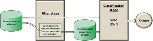
We used a two-stage automatic classifier (Figure 1). The first stage (hereafter referred to as the filter stage) can be an empty filter (in this case, the second stage operates directly on the raw data) or it can be implemented by applying the following techniques over the raw data sequences: down-sampling, feature extraction and normalization. In our application, the down-sampling reduces the frequency of the sequence to 15 Hz (from 30 to 15 data points, five for each accelerometer axis). The feature extraction is applied over each individual accelerometer axis independently. In accordance with Carroll (2014) and Lara (2013), we considered the following features: mean, standard deviation, minimum, maximum, skew, kurtosis, pairwise correlation and overall dynamic body acceleration. We also analyzed the isolated use of only the standard deviation as an input to the second stage. For the normalization, we used a normalization by standard deviation applied to all features extracted. Through these configurations, hereafter, we use: Raw, to represent the dataset of raw accelerometer sequences; Down-sampled, to represent the dataset of down-sampled sequences from the dataset Raw; Standard deviation, to represent the standard deviation computed for each sequence of raw data; Feature extracted, to represent the dataset of features; and Normalized features extracted, to represent the dataset of normalized features. The second stage of the classifier (hereafter referred to as the classification stage) can be based on either SVMs or IDNNs.

Figure 1. The automatic classifier consists of two stages: the filter stage and the classification stage. The raw dataset can be used as direct input to the classification stage, or can be input to the filter stage. The filter stage elaborates the raw dataset, thus generating a preprocessed dataset. The preprocessed dataset is then used as input to the classification stage. The output is the classification of the data, in this case as “prey handling” or “swimming”.

Classification stage

The SVM classifies each sequence of 0.3 s individually. For each sequence, the SVM outputs a positive indicator (1), which identifies prey handling activity, or a negative indicator (−1), identifying swimming activity. We consider three different kernels for the SVM: Linear, Third-Degree Polynomial and RBF. For each kernel, we consider each possible configuration of the filter stage.

The IDNN uses a fully connected network consisting of one input layer, one hidden layer and one output layer, and each neuron of a given layer is connected to all neurons in the previous layer. The number of neurons in the input layer depends on the configuration of the filter stage, and in particular on the number of outputs of this stage. Table 1 shows the number of input neurons for each configuration of the filter stage.

Table 1. The number of neurons that compose an input sequence in each dataset configuration.

Dataset	#Input neurons
Raw (R)	30
Down-sampled (D)	15
Standard deviation (S)	3
Features extracted (F)	22
Normalized Features extracted (FN)	22

We set the number of neurons in the hidden layer at five. This number was selected following an initial analysis of the performance of the IDNN, as described in Section 4.

The output layer is composed of one neuron that classifies each sequence with a number in the range [−1,1], where a positive number means prey handling and a negative number means swimming.

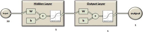
Both the hidden layer and the output layer are implemented with the sigmoidal activation function (Haykin 2009). Figure 2 shows a schema of the IDNN with the raw sequence input.

Figure 2. The IDNN with the raw sequence input of 30 data points. The hidden layer is composed of five neurons and the output layer is composed of one classification neuron.

Validation scheme

The two methods for automatic classification were validated by way of the raw dataset and the filter configurations. Following the procedure described in Section 2.3, the sequences were split randomly by ratio of 70/30, i.e. 3670 training sequences and 1574 testing sequences. The model selection over the two methods was performed with a 10-fold CV approach (Haykin 2009). For each configuration of the filter stage, the model selection phase identifies the best model for each kernel and each learning algorithm. The SVM model is chosen from among the three kernels considered and the value of the C hyper-parameter. The C hyper-parameter was evaluated from the set {0.5, 1, 10, 100}. The IDNN model selection identifies the values for the eta hyper-parameter (η), the alpha hyper-parameter (α) and the lambda hyper-parameter (λ). The η was evaluated from the set {0.1, 0.01, 0.001, 0.0001}. The α and λ are selected from the set {0.0, 0.0001, 0.001, 0.01, 0.1,}.

The maximum number of epochs used for the training phase was identified as the number needed to stabilize the mean squared error (mean squared error) of the IDNN in this phase, resulting in 1000 epochs for the RP learning algorithm and 5000 epochs for the LM and GDM learning algorithms.

Hereafter, best-SVM-‘x’ refers to the SVM with RBF, Linear, or Polynomial that reaches the best average classification accuracy for each configuration of the filter stage. Similarly, best-IDNN-‘x’ refers to the IDNN model trained with RP, LM, or GDM that provides the best average accuracy on an individual configuration filter stage, where ‘x’ is the name of the configuration of the filter stage.

The final accuracy of best-SVM-‘x’ and best-IDNN-‘x’ is obtained by calculating the average accuracy across the generated random splits, retraining and then testing the accuracy of the model five times on each configuration of the dataset.

Experimental results

The experimental results detailed in this paper outline the differences in outcomes between the two models. The different configurations of the models demonstrate the trade-offs between accuracy, memory requested and the need to embed. The experimentation began by selecting the number of hidden neurons for the IDNN. In this analysis, we evaluated the performance of the IDNN with [1–5], 10, 50 and 100 hidden neurons. With more than five neurons, we did not observe meaningful variations in the performance of the IDNN for all considered configurations and for this reason it is apparent that the memory overhead required by more than five hidden neurons is not justified. Table 2 shows the number of weights required by each configuration of the filter stage with 5, 50 and 100 hidden neurons. For the number of neurons within the range of [1–5], the accuracy on the test dataset decreases linearly with the decrease in the number of neurons. We therefore chose a model with five hidden neurons.

Table 2. The quantity of weights for each dataset configuration combined with the different number of hidden neurons is computed by multiplying the number of input neurons in Table 1 with the number of hidden neurons, each weight is eight bytes. For example, an IDNN with a raw data sequence (30 input neurons) and five hidden neurons needs five lots of 30 weights for the hidden layer.

Dataset	5 hidden neurons	50 hidden neurons	100 hidden neurons
R	150	1500	3000
D	75	750	1500
S	15	150	300
F	110	1100	2200
FN	110	1100	2200

Next, we analyze the results from two points of view. For the first, we focus our attention on the performance obtained with each combination of configuration of dataset and models. For the latter, we analyze the same performances but with attention to the configurations.

In accordance with the validation scheme presented in 3.2, we selected a model for each configuration of the first stage. We analyzed the results obtained with the selected model, from the lowest accuracy to the highest. The analysis below is in reference to the results shown in Figure 3. More details and results obtained with the test dataset of each configuration are listed in Table 3.

Table 3. Shown here is the memory required for each best-SVM-x and best-IDNN-x configuration as well as their corresponding accuracy. The second column lists the memory required by the SVM for each selected model, and the same applies for the IDNN in the third column. The memory is in kilobytes. The fourth column gives the accuracy provided by the selected models of SVM and the fifth by the selected models of IDNN.

Dataset	SVM memory requirement (kB)	IDNN memory requirement (kB)	SVM accuracy	SVM F1score	IDNN accuracy	IDNN F1score
R	1169	1	81.7%	81.1%	79.2%	79.5%
			(± 0. 003)	(±0.0028)	(± 0. 008)	(± 0. 008)
D	403	0.6	79.8%	80.5%	78.1%	78.5%
			(± 0.005)	(±0.0020)	(± 0.004)	(±0.0064)
S	40	0.11	75.7%	86.2%	76.5%	85.9%
			(± 0.018)	(±0.0000)	(± 0.004)	(±0.0036)
F	214	0.85	84.5%	90.1%	85.2%	90.5%
			(± 0.006)	(±0.0007)	(± 0.005)	(±0.0036)
FN	222	0.8	84.9%	90.4%	84.5%	90.1%
			(± 0.005)	(±0.0005)	(± 0.004)	(±0.0037)

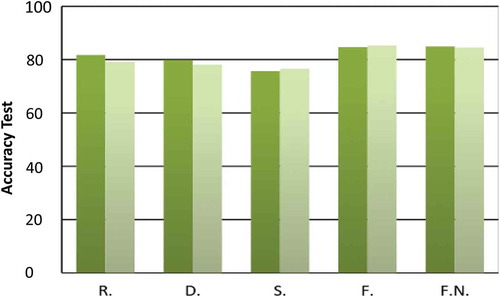
Figure 3. This figure shows the accuracy achieved with the selected model for SVM and IDNN for each configuration of the first stage. The horizontal axis denotes the acronyms referring to each given configuration: Raw (R), Down-sampled (D), Standard deviation (S), Features extracted (F) and Normalized Features extracted (F.N.). The vertical axis displays the accuracy. Light green represents the accuracy of best-IDNN-’x’, and dark green the accuracy of best-SVM-’x’.

In our experimental results, we found an optimal accordance among the results obtained with the training, validation and test datasets. The difference between the three is respectively about 0.9*10^–2, 1.1*10^–2, and between 0.1*10^–2 and 0.5*10^–2, for the five different configurations of the dataset This is indicative of a good reliability providing a proof of the consistency of the learning phases. Table 3 shows the results obtained over the test dataset.

The accuracy of the different configurations was broadly similar among all IDNN models (on the RP, LM and GDM). A more noticeable difference can be seen between the SVM in the Linear kernel and the Raw dataset, as well as the Polynomial kernel and Features extracted dataset. In these cases, the accuracy decreases by up to 10%, depending upon which model is selected. We selected and presented the best model for each configuration.

For the standard deviation dataset, the best-SVM-S model is the SVM with RBF kernel with C = 1 and the best-IDNN-S is selected as an IDNN trained with RP with η = 0.001 and λ = 0.0001. Both models selected provide a similar accuracy, but the accuracy obtained with best-IDNN-S was slightly higher (by 1%) than the best-SVM-S.

For the down-sampled dataset, we observed a small difference in the results of the two models selected for SVM and IDNN. The validation procedure identifies the best-SVM-D to be an SVM with a Polynomial kernel with C = 1, and for the same procedure, the best-IDNN-D is identified as the IDNN trained with the LM algorithm. The best-SVM-D provides a slightly higher accuracy (79%) compared with the accuracy obtained with best-IDNN-D (78%).

The SVM performed better than the IDNN with the original raw dataset. In particular, the SVM with the RBF kernel (best-SVM-R) with C = 1 was accurate at a rate of 81.7%, whereas the IDNN trained with the RP with η = 0.01 and λ = 0.001 (best-IDNN-R) was accurate at the rate of 79%. In this case, the difference of accuracy is 2%. However, this level of difference does not have a significant impact on the final results of the program. For the dataset with the features extracted, as well as with normalized features extracted, both the SVM and the IDNN achieved a rate of accuracy of approximately 84.9%. The best-SVM-F is an SVM with a polynomial kernel and C = 100, achieving an accuracy of 84.9% – the result presented in the previous study using this dataset (Carroll 2014). The model selected for best-IDNN-F is IDNN trained, with RP, and with η = 0.1 and λ = 0.01. This model provides a higher accuracy than best-SVM-F by 0.1% (85%), but this difference is not of statistical significance for this analysis. A similar result is obtained for the model selected with the normalized features. In this case, best-SVM-FN, selected as an SVM with a Linear kernel and C = 100, achieves 85% accuracy, and the IDNN with RP, and with η = 0.1 and λ = 0.01 (best-IDNN-FN), achieves 84.5% accuracy.

We observed that the performances obtained for the best-SVM-x and the best-IDNN-x models were almost identical for each configuration of the filter stage. This observation is confirmed primarily when taking into consideration the f1score (Table 3). The results obtained for this measurement were in accordance with the corresponding accuracy performance.

In Table 3, the standard deviation computed for each configuration was lower than the difference between the SVM model and the IDNN model. The standard deviation was therefore not used as an important factor influencing our comparison between models based on either overall accuracy or f1score.

The key advantage of using the IDNN, over the SVM, is the low quantity of memory required for the model to operate. The trained IDNN model requires memory for the input sequence as well as for the weights. For each IDNN configuration, the number of weights is computed as the length of the input sequence multiplied by the number of neurons in the hidden layer. The number of samples for the input sequence (represented in the input vector) varies according to the configuration of the filter stage (Table 1). The number of neurons for the hidden layer is fixed at five neurons (as explained in Section 5.2).

The trained SVM model requires memory to store the support vectors. The dimension of each support vector is related to the dimension of the input sequence. The number of support vectors is computed during the training phase. Table 4 shows the number of support vectors and their dimension for each best-SVM-x identified during the validation procedure. Given the number of support vectors and their dimension, we compute the memory required for each selected model.

Table 4. The table lists the number of support vectors identified for each selected model of SVM. The first column is the selected model. The second column is the number of support vectors identified for the current model. The third column lists the dimension for each SV.

Selected model for configuration	#support vectors (SV)	Dimension of SV
Best-SVM-R	4991	30
Best-SVM-D	3441	15
Best-SVM-S	1731	3
Best-SVM-F	1248	22
Best-SVM-FN	1292	22

The support vectors and weights consist of vectors of double numbers (8 Bytes per number).

Given that the IDNN model uses so much less memory than the SVMs, while achieving almost identical levels of accuracy, the preferred choice for the identification of prey handling activities in this situation is the IDNN.

Table 3 shows a summary of the memory requirement (in kilobytes), as well as the accuracy achieved for each configuration of the filter stage for each model.

In Figure 3, we observe that the accuracy obtained with both best-SVM-x and best-IDNN-x is similar with each configuration of the first stage. Despite this, the memory requirements for the IDNN model are significantly lower than the corresponding SVM configuration. Note that the best-SVM-x has an inherent memory requirement due to its need to keep memory for the selected support vectors. In the following paragraph, we discuss the ratio between accuracy achieved and memory required.

For the raw dataset, the memory usage of best-IDNN-R was 1 kB, which is more than 1000% less than the memory required by the best-SVM-R. The IDNN allows us to reduce the memory usage to 1 kB, but incurs a reduction in accuracy of 2% (from 81% to 79%).

A similar advantage is observed with the down-sampling configuration. The IDNN selected model requires only 0.5 kB instead of 403 kB, with a mere 1% penalty in accuracy.

For the raw and down-sampled dataset, the advantage of using IDNN in terms of memory usage is self-evident. Despite the marginal accuracy disadvantage, the low memory usage of the IDNN model makes it ideal for embedding on a device. A smaller difference in memory requirement is observed for the standard deviation, feature extracted and normalized feature extracted configurations.

For the standard deviation configuration, we observed an accuracy increase of only 1% in the best-IDNN-s, while the memory usage for this model is only 0.11 kB. This space requirement is more than fifty times less than the memory required by the best-SVM-s. For both plain and normalized features extracted configurations, the SVM model requires 214 kB. The IDNN model, however, only requires 0.8 kB. As before, the percentage of accuracy lost with the IDNN is not significant enough, especially when considering how much memory is saved by using the IDNN.

The memory requirement for the SVM, regardless of the configuration, can be anywhere from 40 to 1169 kB. It influences how to choose the model for the embedded design. The IDNN, on the other hand, requires less than 1 kB of data for any given configuration.

Concerning the dataset configurations, with both the IDNN and SVM models, we observe a significant difference in performance depending on the specific dataset in use. This difference is highlighted in Figure 4. Specifically, Figure 4a shows the performance versus the normalized memory occupation of the IDNN model applied to the five datasets. From the figure, it is seen that the best performance with high memory occupation is achieved on the feature extracted dataset, as proposed in Carroll (2014). On the other hand, this configuration requires the selection and computation of features over each sequence. This affects the flexibility of the approach, since the selection of the features is an ad hoc process that should be repeated whenever this solution is applied to another use case (e.g. if this solution is applied to a dataset obtained from different species of penguin). A similar consideration holds in the case of IDNN with normalized feature extracted dataset. Concerning the IDNN applied to the raw dataset, we observe that this solution achieves an average performance (with only a 3% penalty in accuracy with respect to IDNN with the feature dataset) and the highest, but still very low (1 kB), memory occupation. On the other hand, this solution is the most flexible since it does not require any ad hoc adaptation to determine the best features if applied to other use cases. The down-sampled and standard deviation datasets offer a compromise between the two extreme cases of IDNN with raw and IDNN with features extracted cases. Considering however that the penalty in memory occupation is always very low (at most 1 kB) for all the cases, the choice of the most appropriate solution for a specific use case is determined by the trade-off between performance/flexibility.

Figure 4. Normalized memory occupation versus accuracy for the different datasets and models. Figure 4a refers to the IDNN model applied to the different datasets, and the memory occupation is normalized assuming 1 to be 1 kB. Figure 4b refers to the SVM model applied to the different datasets, and the memory occupation is normalized assuming 1 be 1 mB.

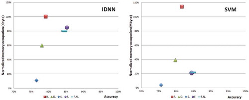
Concerning SVMs, Figure 4b shows the performance versus the normalized memory occupation of the SVM model applied to the five datasets. In this case, the best performance is achieved on the feature extracted and normalized feature extracted dataset (both with a moderate memory occupation). Instead, the SVM with raw dataset achieves similar performances with a significantly higher memory occupation. The down-sampled and standard deviation datasets offer a compromise between memory occupation and performance. When considered from the point of view of flexibility of the solution, we observe that the cost for flexibility for SVM is in terms of a penalty for both memory and performance. If flexibility is a strong requirement, but the solution of SVM with the raw dataset is not appropriate, then a valid option is given by using an SVM with a down-sampled dataset. The SVM applied to a standard deviation dataset is outperformed by all IDNN approaches and configurations, and can thus be disregarded.

Conclusion

Our study applied, evaluated and compared the SVM and IDNN models, in order to optimize the trade-off among memory requirements, classification accuracy and generality of the models for classifying activity from acceleration data. For this purpose, we compared the settings for SVM and IDNN classifiers at both the filter stage and the classification stage. We show that in all cases, the IDNN models have lower memory requirements than the SVM models, with similar classification accuracy. We further show that by adjusting the settings, it is possible for researchers to choose between IDNN models that focus either on high accuracy or on high generality depending on the priorities of their research.

In some cases, achieving high classification accuracy is of the greatest importance. In our experiments, this is achieved with a score of 85% (f1score of 90%) by the ‘extracted features’ configuration IDNN. For this approach, the filter stage configuration is the features extracted dataset. It is necessary to select a set of features to represent patterns in the raw data as well as to compensate for the potential loss of some information. The features are selected ad hoc and the selection of these features should be optimized for each new task. The extraction of features needs to be computed over each sequence requiring additional memory and time. This result is mainly of interest in cases where the autonomous classifier is applied to a specific problem with wide limits in memory and time, and the generality of the system to other cases is not expected.

In some cases, generalizability of the model to different scenarios is important. In our study, we developed a more generalizable model that achieved a moderate accuracy of 81%. In this case, it is not necessary to perform an ad hoc selection of features. No filters are applied and the entire data stream is used with the complete information of the signal. This allows a model of the classification stage to be generalizable over other raw datasets.

The low memory requirements and high accuracy of the IDNN model suggest that it is a promising method for classifying the activity of wild animals from accelerometry data. Previously, the identification of prey handling events by little penguins using an SVM showed that the rate and spatial location of feeding events could be accurately identified in this species from patterns in their acceleration profile (Carroll 2014, Carroll et al. 2016). As little penguins return reliably to the nest during the breeding season, the ability to download logged data streams precluded the need for extensive data compression and onboard processing in these earlier studies. However, not all field studies have the option of retrieving the biologger. The advantage identified in this study is that the IDNN models achieve similar accuracy to the SVM, but are better suited for analyzing the behavior of animals that do not return to shore regularly, or that are difficult to recapture (e.g. seabirds outside the breeding season, seals, dolphins and fish). In such cases, the data must undergo some embedded processing before being uploaded to a server for remote access.

Collection, storage and transmission of data are constrained by power and memory requirements, which are in turn limited by the size of devices that can be attached to the animals. Data transmitters therefore require significant data compression to reduce both size and power requirements. For instance, in the widely used ARGOS animal tracking service, uplinks may contain a maximum of only 256 bits (32 bytes) per message in a rigid format (Fedak 2002). In this case, application of the IDNN provides a significant step toward onboard processing, followed by the remote upload of time-coded animal behavior labels from almost anywhere on the planet. With an IDNN system directly installed on the onboard tag, it is possible to acquire information about the animals and analyze them on-site, thus monitoring the animal in real time.

The adoption of supervised machine learning approaches to use labeled behavior data for learning is challenging for marine species that are not kept in captivity, or cannot simultaneously have a camera and accelerometer attached. However, for those species where this approach is feasible and the accuracy of behavior classifications can be determined, the ability to subsequently store and transmit reliable behavior labels provides a powerful tool. The research in this paper indicates that the anticipated future developments of onboard processing algorithms and the associated tag hardware will lead to an increasing adoption of accelerometers across a wide range of fields of animal ecology.

References

- Augustin, A., J. Yi, T. Clausen, and W. M. Townsley. 2016. A study of LoRa: Long range & low power networks for the internet of things. Multidisciplinary Digital Publishing Institute 16:9.
- Barbuti, R., S. Chessa, A. Micheli, and R. Pucci. 2016. Localizing tortoise nests by neural networks. PlosOne 11:e0151168. doi:10.1371/journal.pone.0151168.
- Baylis, A. M., R. A. Orben, P. Pistorius, P. Brickle, I. Staniland, and N. Ratcliffe. 2015. Winter foraging site fidelity of king penguins breeding at the Falkland Islands. Marine Biology 162. doi:10.1007/s00227-014-2561-0.
- Broell, F., T. Noda, S. Wright, P. Domenici, J. F. Steffensen, J. P., Auclair, and C. T. Taggart. 2013. Accelerometer tags: Detecting and identifying activities in fish and the effect of sampling frequency. Journal of Experimental Biology 216:1255–64. doi:10.1242/jeb.077396.
- Burton, R. K., and P. L. Koch. 1999. Isotopic tracking of foraging and long-distance migration in northeastern Pacific pinnipeds. Oecologia 119:578–85. doi:10.1007/s004420050822.
- Carroll, G., J. D. Everett, R. Harcourt, D., Slip, and I. Jonsen. 2016. High sea surface temperatures driven by a strengthening current reduce foraging success by penguins. Scientific Reports 6. doi:10.1038/srep22236.
- Carroll, G., D. Slip, I. Jonsen, and R. Harcourt. 2014. Supervised accelerometry analysis can identify prey capture by penguins at sea. Journal of Experimental Biology 217:4295–302. doi:10.1242/jeb.113076.
- Cury, P. M., I. L. Boyd, S. Bonhommeau, T. Anker-Nilssen, R. J. Crawford, R. W. Furness, J. A. Mills, E. J. Murphy, H. Österblom, M. Paleczny, and J. F. Piatt. 2011. Global seabird response to forage fish depletion—One-third for the birds. Science 334:1703–06. doi:10.1126/science.1212928.
- Davis, R. W. 2008. Bio-logging as a method for understanding natural systems. Informatics Education and Research for Knowledge-Circulating Society. ICKS, Kyoto, Japan.
- Davis, R. W., L. A. Fuiman, T. M. Williams, S. O. Collier, W. P. Hagey, S. B. Kanatous, S. Kohin, and M. Horning. 1999. Hunting behavior of a marine mammal beneath the Antarctic fast ice. Science 283:993–96. doi:10.1126/science.283.5404.993.
- Dubois, Y., G. Blouin‐Demers, B. Shipley, and D. Thomas. 2009. Thermoregulation and habitat selection in wood turtles Glyptemys insculpta: Chasing the sun slowly. Journal of Animal Ecology 78:1023–32. doi:10.1111/jae.2009.78.issue-5.
- Escalante, H. J., S. V. Rodriguez, J. Cordero, A. R. Kristensen, and C. Cornou. 2013. Sow-activity classification from acceleration patterns: A machine learning approach. Computers and Electronics in Agriculture 93:17–26. doi:10.1016/j.compag.2013.01.003.
- Eston, R. G., A. V. Rowlands, and D. K. Ingledew. 1998. Validity of heart rate, pedometry, and accelerometry for predicting the energy cost of children’s activities. Journal of Applied Physiology 84:362–71.
- Fedak, M., P. Lovell, B. McConnell, and C. Hunter. 2002. Overcoming the constraints of long range radio telemetry from animals: Getting more useful data from smaller packages. Integrative and Comparative Biology 42:3–10. doi:10.1093/icb/42.1.3.
- Fletcher, R. 2013. Practical methods of optimization. John Wiley & Sons.
- Foo, D., J. M. Semmens, J. P. Arnould, N. Dorville, A. J. Hoskins, K. Abernathy, G. J. Marshall, and M. A. Hindell. 2016. Testing optimal foraging theory models on benthic divers. Animal Behaviour 112:127–38. doi:10.1016/j.anbehav.2015.11.028.
- Francis, L. A., and K. Iniewski. 2013. Novel advances in microsystems technologies and their applications. CRC Press.
- Gao, L., H. A. Campbell, O. R. Bidder, and J. Hunter. 2013. A Web-based semantic tagging and activity recognition system for species’ accelerometry data. Ecological Informatics 13:47–56. doi:10.1016/j.ecoinf.2012.09.003.
- Gemma, C., D. Slip, I. Jonsen, and R. Harcourt. 2014. Supervised accelerometry analysis can identify prey capture by penguins at sea. Journal of Experimental Biology 217:4295–4302.
- Gill, P. E., and W. Murray. 1978. Algorithms for the solution of the nonlinear least-squares problem. SIAM Journal on Numerical Analysis 15:977–92. doi:10.1137/0715063.
- Grant, M., S. Boyd, and Y. Ye. 2008. CVX: Matlab software for disciplined convex programming.
- Haykin, S. 2009. Neural networks and learning machines, 3rd ed. NJ, USA: Pearson Upper Saddle River.
- Heaslip, S. G., W. D. Bowen, and S. J. Iverson. 2014. Testing predictions of optimal diving theory using animal-borne video from harbour seals (Phoca vitulina concolor). Canadian Journal of Zoology 92:309–18. doi:10.1139/cjz-2013-0137.
- Hussey, N. E., S. T. Kessel, K. Aarestrup, S. J. Cooke, P. D. Cowley, A. T. Fisk, R. G. Harcourt, K. N. Holland, S. J. Iverson, J. F. Kocik, and J. E. M. Flemming. 2015. Aquatic animal telemetry: A panoramic window into the underwater world. Science 348:1255642. doi:10.1126/science.1255642.
- Kays, R., M. C. Crofoot, W. Jetz, and M. Wikelski. 2015. Terrestrial animal tracking as an eye on life and planet. Science 348:aaa2478. doi:10.1126/science.aaa2478.
- Lara, O. D., and M. A. Labrador. 2013. A survey on human activity recognition using wearable sensors. IEEE Communications Surveys\& Tutorials 15.
- Miyashita, K., T. Kitagawa, Y. Miyamoto, N. Arai, H. Shirakawa, H. Mitamura, T. Noda, T. Sasakura, and T. Shinke. 2014. Construction of advanced biologging system to implement high data-recovery rate-a challenging study to clarify the dynamics of fish population and community. Nippon Suisan Gakkaishi 80:1009–15. doi:10.2331/suisan.80.1009.
- Montoye, H. J., R. Washburn, S. Servais, A. Ertl, J. G. Webster, and F. J. Nagle. 1982. Estimation of energy expenditure by a portable accelerometer. Medicine and Science in Sports and Exercise 15:403–07.
- Morè, J. J. 1978. The Levenberg-Marquardt algorithm: Implementation and theory. Numerical Analysis, 105–116.
- Nathan, R., O. Spiegel, S. Fortmann-Roe, R. Harel, M. Wikelski, and W. M. Getz. 2012. Using tri-axial acceleration data to identify behavioral modes of free-ranging animals: General concepts and tools illustrated for griffon vultures. Journal of Experimental Biology 215:986–96. doi:10.1242/jeb.058602.
- Owen, K., R. A. Dunlop, J. P. Monty, D. Chung, M. J. Noad, D. Donnelly, A. W. Goldizen, and T. Mackenzie. 2016. Detecting surface-feeding behavior by rorqual whales in accelerometer data. Marine Mammal Science 32(1):327–48.
- Payne, N. L., M. D. Taylor, Y. Y. Watanabe, and J. M. Semmens. 2014. From physiology to physics: Are we recognizing the flexibility of biologging tools? Journal of Experimental Biology 217:317–22. doi:10.1242/jeb.093922.
- Riedmiller, M. 1994. Advanced supervised learning in multi-layer perceptrons—From backpropagation to adaptive learning algorithms. Computer Standards & Interfaces 16:265–78. doi:10.1016/0920-5489(94)90017-5.
- Roland, K., M. C. Crofoot, W. Jetz, and M. Wikelski. 2015. Terrestrial animal tracking as an eye on life and planet. Science 348:aaa2478. doi:10.1126/science.aaa2478.
- Shaughnessy, P. D., R. J. Kirkwood, and R. M. Warneke. 2002. Australian fur seals, Arctocephalus pusillus doriferus: Pup numbers at Lady Julia Percy Island, Victoria, and a synthesis of the species’ population status. Csiro 29(2):185–92.
- Soltis, J., R. P. Wilson, I. Douglas-Hamilton, F. Vollrath, L. E. King, and A. Savage. 2012. Accelerometers in collars identify behavioral states in captive African elephants Loxodonta africana. Endangered Species Research 18:255–63. doi:10.3354/esr00452.
- Sutton, G. J., A. J. Hoskins, and J. P. Arnould. 2015. Benefits of group foraging depend on prey type in a small marine predator, the little penguin. PlosOne 10:e0144297. doi:10.1371/journal.pone.0144297.
- Vapnik, V. 1998. Statistical learning theory. New York: Wiley.
- Volpov, B. L., A. J. Hoskins, B. C. Battaile, M. Viviant, K. E. Wheatley, G. Marshall, K. Abernathy, and J. P. Arnould. 2015. Identification of prey captures in Australian fur seals (Arctocephalus pusillus doriferus) using head-mounted accelerometers: Field validation with animal-borne video cameras. PlosOne 10:e0128789. doi:10.1371/journal.pone.0128789.
- Wilson, A. D., M. Wikelski, R. P. Wilson, and S. J. Cooke. 2015. Utility of biological sensor tags in animal conservation. Conservation Biology 29:1065–75. doi:10.1111/cobi.2015.29.issue-4.
- Wilson, R. P., and C. R. McMahon. 2006. Measuring devices on wild animals: What constitutes acceptable practice? Frontiers in Ecology and the Environment 4:147–54. doi:10.1890/1540-9295(2006)004[0147:MDOWAW]2.0.CO;2.
- Yasuda, I., H. Sugisaki, Y. Watanabe, S. S. Minobe, and Y. Oozeki. 1999. Interdecadal variations in Japanese sardine and ocean/climate. Fisheries Oceanography 8:18–24. doi:10.1046/j.1365-2419.1999.00089.x.