Evaluation of Naive Bayes and Support Vector Machines for Wikipedia

ABSTRACT

Wikipedia has become the de facto source for information on the web, and it has experienced exponential growth since its inception. Text Classification with Wikipedia has seen limited research in the past with the goal of studying and evaluating different classification techniques. To this end, we compare and illustrate the effectiveness of two standard classifiers in the text classification literature, Naive Bayes (Multinomial) and Support Vector Machines (SVM), on the full English Wikipedia corpus for six different categories. For each category, we build training sets using subject matter experts and Wikipedia portals and then evaluate Precision/Recall values using a random sampling approach. Our results show that SVM (linear kernel) performs exceptionally across all categories, and the accuracy of Naive Bayes is inferior in some categories, whereas its generalizing capability is on par with SVM.

Introduction

Classification is a machine learning technique for assigning labels to unseen data based on models built using an algorithm and labeled data. It consists of a training phase and a testing phase. Classification is also considered as a supervised learning technique because of the presence of a training phase. It can be performed on any type of data – text, images, videos, web data, numbers, etc. Text classification deals with text data and more specifically classifying a corpus of documents. In this context, Wikipedia offers an excellent case study for evaluating classifiers over a large and varied dataset.

We first discuss the prior work on leveraging Wikipedia directly and indirectly for classification. Then, we describe two prominent text classification algorithms – Naive Bayes and Support Vector Machines (SVMs). Finally, we describe the implementation and the results obtained using both these classifiers, using two metrics indicative of the accuracy and completeness of the documents retrieved. In our paper, we use the terms articles and documents interchangeably.

Related work

In most previous works, Wikipedia has been used to supplement and add context to the text classification of different datasets, rather than Wikipedia being the direct target of the classification problem. Wang et al. (2009) discuss the process of building a thesaurus from Wikipedia to be leveraged in the text classification of documents. Wang and Domeniconi (2008) built semantic kernel representation from Wikipedia thesauruses for improving text classification accuracy and compared it with the Bag of Words (BoW) representation. Wikipedia has also been used as a knowledge base to tag, extract entities, and classify social media information (tweets) (Gattani et al. 2013). These papers have addressed general text classification problems with Wikipedia as a valuable tool for additional context. However, there hasn’t been significant research in treating Wikipedia itself as the target for classification. This paper aims to make significant progress in that regard. Mehdi et al. (2017) published a summary of how the Wikipedia corpus has been leveraged directly/indirectly for various purposes in research, including text classification, which is of interest to us. Murugeshan, Lakshmi, and Mukherjee (2009) put forward a novel approach of combining classifiers exploiting Wikipedia’s structure and using different similarity metrics. Although this approach produces exceptional accuracy, the generalization capability seems to be relatively low overall, as indicated by the F-score values. We show that an individual classifier like SVM can achieve high Recall scores without significant hit in Precision.

Wikipedia is a massive dataset, and the classification of large datasets is a major challenge. Parallel processing leveraging supercomputers has been used to construct custom Decision tree classifiers for the fast processing of classification of large datasets (Joshi, Karypis, and Kumar 1998). An efficient forest-based algorithm has been built for the fast classification of large datasets (Fãbio et al. 2010). In our work, we limit our focus to the accuracy and completeness of the classification process rather than general performance.

Naive Bayes

Naive Bayes is a probabilistic learning algorithm, and its simplicity is rooted in the assumption that the features of the underlying data are independent of each other. Despite its simplicity and this assumption failing in many cases, it produces surprisingly accurate results. In the text classification context, this would mean that all the words in a document are independent of each other. For a given training set, a vocabulary is built from the words in the corpus and probabilities are computed for each word belonging to a particular class. Using these computed probabilities, test documents are classified by applying the Bayes rule and determining the class having a higher probability, which turns out to be the decision class. How the probabilities are computed and the Bayes rule is applied depend on the underlying event model used. Two widely known event models are used for Naive Bayes – the Bernoulli (Binomial) model and the Multinomial model.

Bernoulli model

In the Bernoulli model, the vocabulary is built from the training corpus and each document (test or training) is modeled in the context of a word’s existence in the document. We can define it in mathematical terms as follows. Consider a vocabulary with words created from a training set. A test document with words can be represented as a vector of zeros and ones, where is 1 if the word is part of the vocabulary and 0 if not. In the training phase, for each word w in the vocabulary, we compute the conditional probability given a class. Once these conditional class probabilities are computed, in the test phase, we compute the product of all such probabilities for each word in the test document.

Because the number of words in a document could be substantial, the products of so many probabilities could lead to floating point underflow. To avoid this, probabilities are stored on a logarithmic scale. The Bernoulli model works well for small vocabulary sizes, but when the vocabulary size exceeds 1000 words, it fails to take enough information into account (frequencies) to make accurate predictions (McCallum et al. 1998). Because Wikipedia documents are typically large and our vocabulary for each of the categories exceeds the optimal limit for the Bernoulli model (McCallum et al. 1998), we did not proceed with it and instead opted for the more appropriate Multinomial model.

Multinomial model

The Multinomial model encodes more information than just the existence or absence of any particular word. In the context of Wikipedia classification, this attribute becomes very useful. For example, consider the “Astronomy” category. An article belonging to this category is likely to have keywords like “Galaxy,” “Star,” “Space,” etc. Therefore, the vocabulary built from the training set will have higher frequencies (or weights) for such domain-specific keywords and result in higher probabilities for these keywords. This also increases the likelihood of correctly classifying an “Astronomy” article. In contrast, the Bernoulli model assigns equal weights (1) to words that exist, even if they occur multiple times. We now proceed to define the Multinomial model in mathematical terms as follows with some of the terms carried forward from the Bernoulli model (Manning, Raghavan, and Schütze 2008).

vocabulary, extracted by tokenizing the documents in the training corpus

i^th class from a set of classes

probability of the i^th word occurring for a given class

number of words in vocabulary

frequency/count of word in documents belonging to class

(1)

To avoid cases of zero probabilities, we include the “1” term, which is referred to as Laplacian Smoothing. To compensate for this, the vocabulary size is included in the denominator.

probability of class c given a document D

W = extracted tokens from document D

prior probability of class c

(2)

(3)

(4)

As seen in Eqs. (1)–(4), we determine the posterior probabilities for a test document and choose the class with the maximum probability (also called the Maximum Posterior Estimate).

Naive Bayes is a linear classifier in that the decision boundary separating the classes (in a binary classification problem) is linear. Although efficient and simple to implement, the independence assumption can produce false positives (FPs). For example, articles related to science fiction could be classified as “Astronomy” as words are considered independently and the semantic relationship (phrases or sentences) is ignored. However, as we observe in the results, this assumption works surprisingly well for a few categories at least, especially whose domain-specific keywords are overall unique to Wikipedia with insignificant overlap with other categories.

We also implemented some optimizations to Naive Bayes – removing words with counts below a certain threshold and filtering unrelated keywords manually. However, these adjustments did not offer much improvement in accuracy and in some cases made it worse.

SVMs

SVMs take a fundamentally different and sophisticated approach to classifying documents. It treats classification as primarily an optimization problem. To be more specific, we consider documents represented in a higher-dimensional space. The optimization problem basically involves finding the maximal “hyperplane,” i.e. a plane in higher dimensional space separating the documents of different classes, and the degree of separation between the classes is to be maximized subject to minimizing the error. The type of hyperplane depends on the “kernel” used to compute weights for the training examples. Kernels can be linear, radial (RBF), or polynomial. Text categorization problems are generally linearly separable, and as a result we only consider SVMs with linear kernels in this study. SVM is defined formally as in Eqs.(5)–(7):

training documents of m-dimensions

and = classes of a binary classifier

(5)

The hyperplane equation is then given by

(6)

Here, w is the vector normal to the hyperplane and b is the bias term added so that optimal hyperplane can be found, as a hyperplane passing through the origin need not necessarily be the one with the maximum margin.

The margin is given by . This needs to be maximized, which in turn means needs to be minimized. The problem can then be framed as a quadratic optimization problem subject to a constraint, as defined below.

(7)

The constraint is that the actual training label and the predicted label must have the same sign, i.e. the same class. The above Quadratic Program (QP) can be solved using any standard solver, by converting it to the Lagrangian form and then finding the multipliers/weights.

This is also called the hard margin classifier and works well in the case of perfect linearly separable classes. As a result, it does not offer flexibility for any violations. With Wikipedia being so large, it can be assumed that our training set is not completely representative of all possible articles for a category. Hence, having some violations of the maximal hyperplane is acceptable, and to this end, we use the soft margin classifier. The soft margin introduces a regularization parameter C, which controls the degree of misclassification allowed, and the optimization problem is modified to accommodate a “slack term” (Cortes and Vapnik 1995).

(8)

Here, the s are called slack terms. In the Lagrangian form, the multipliers become bounded by C rather than being unbounded in the hard margin classifier. In our evaluation, we discuss the effects of varying C on the recall/generalization capability of the model.

Document representation

The massive size of Wikipedia in its raw representation has been well documented (Denoyer et al. 2006). We consider only the English version of Wikipedia for the scope of this problem. The Wikipedia raw data is stored in a custom XML format called MediaWiki. An article and its metadata are encoded within page tags. Within a page, we can infer the article’s title, raw text, ID, and the history of revisions. The sequence of pages is ordered by article ID. We only consider the title and raw text for classifying the articles. To be able to build a classification model, we need to be able to translate the text content to a mathematical representation, which can be used in either computing the probabilities for Naive Bayes or computing the Lagrange multipliers in case of SVM.

The raw article text is annotated with several Wikipedia-specific tags relating to images, URLs, and tables contained within the article. As such, this mostly serves as noise, and extracting plain text free of noise is not straightforward. In our experiments, we perform naive preprocessing. Figure 1 illustrates the steps involved. Non-alphanumeric characters are removed and then tokenization is performed with whitespace as delimiter. Apart from basic English stop words, we also have common Wikipedia words (part of annotated tags) included in this list as they are not domain-specific. To deal with different forms of a word (verb, adverb, plurals, etc.) and with the goal of consolidating such different instances, we perform stemming, which extracts the word root and stores it as part of the vector. Alternatively, lemmatization can also be carried out if semantic meaning has to be preserved. Porter stemmer is one of the standard stemming algorithms that we leverage here.

Figure 1. Steps involved in feature extraction from Wikipedia documents.

After stemming, we use different representations for Naive Bayes and SVM, allowing for the best possible results in terms of accuracy and completeness. For Naive Bayes, we employ the BoW model as discussed in previous sections and store the word along with its count across the training documents in a dictionary. For SVM, term frequency-inverse document frequency (tf-idf) representation works better than raw counts (McCallum 1998). The tf-idf scoring is defined in several ways (log normalized/smoothed/probabilistic), for a word is defined as in Eqs.(9)–(11):

i^th word in document d

corpus or set of all training documents

term-frequency of word in document

inverse document-frequency of a word in corpus

number of occurrences of word in document

number of documents in corpus D in which the word occurs

(9)

(10)

(11)

Documents are thus represented in m-dimensional space (m is the number of words in vocabulary) as a vector of tf-idf scores and used in the SVM learning process to determine the optimal hyperplane.

Results

We now discuss the evaluation of the above-mentioned models for six different categories – Astronomy, Dance, Economics, Religion, Psychology, and Computer Science. These subjects were chosen because they are significantly diverse in their vocabulary and as a result useful to project any conclusions regarding the behavior of the classifiers to the Wikipedia as a whole. The training data was chosen for some subjects using subject matter experts, and in their absence, Wikipedia Portals.

Wikipedia has portal sections for many subjects/areas, which have links and lists of articles that might be pertaining to that subject. Classification for each category is treated as an independent binary classification problem (one versus others) rather than a multi-label classification problem, for the sake of simplicity. Thus, the classification problem for Astronomy would have two labels “Astronomy” and “Not Astronomy.” We also collect articles reflective of the latter label from Wikipedia for the training set, and this also applies to other categories. The training set sizes for all the categories are around 300–350 articles. In case of SVM, we have more articles as part of the training set (compared to Naive Bayes) as it has been demonstrated that SVM performs better with more features (Joachims 1998).

Wikipedia data is available as XML in compressed bz2 formats^, provided by the Wikimedia foundation on their website. It can be accessed as a single large file or a series of partitions numbered up to 27. The latter becomes useful in evaluation for sampling. Our evaluation covers only linear SVM and Multinomial Naive Bayes.

Precision and Recall

Precision and Recall are two important metrics that can be used to evaluate a binary classifier. Precision indicates the degree to which the documents that were retrieved were relevant. Recall, on the other hand, indicates the degree to which relevant documents were retrieved from all the documents in the corpus. We use both metrics for all the binary classification problems defined for the categories for comparison.

Evaluating Precision and Recall for a binary classifier generally involves sampling unseen data and feeding them to the classifier. Some of the common sampling strategies are holdout, k-fold cross-validation, Leave-p-out cross-validation, etc. We use a different but straightforward sampling method more suited to the vast and varying nature of the Wikipedia data.

1. For evaluating Precision, we take numerous samples of fixed size (e.g. 100) per a fixed number of retrieved documents (e.g. 2000) provided by the classifier (over the whole Wikipedia dataset). These documents were then manually checked to determine the true positives (TPs) and FPs. This strategy is repeated for all categories and both classifiers.

2. Recall, on the other hand, is much more challenging to evaluate as it requires sampling over a much larger set (a substantial fraction of the whole Wikipedia). Accordingly, we adopt a different sampling approach involving only the partitions of the Wikipedia. From each of the partitions (27), we randomly sample 10 sets of samples, with each sample consisting of 200 articles. After the classification of the sampled articles, Recall is computed over each sample and the values are averaged to obtain the representative value.

Precision and Recall are calculated based on the following equations:

(12)

where true positives

and false positives

(13)

where = false negatives.

All our experiments were performed on a machine with Intel Core i7 processor (2.8 GHz) and Ubuntu OS. We implemented Naive Bayes algorithm in Java, along with a SAX parser for parsing the Wikipedia XML. For preprocessing the data, we have stop word removal with typical English stop words and some common Wikipedia-specific terms, which also serve as noise. Some of these terms are HTML/XML tags for accommodating tables, lists, and URLs within the article. Stemming is also leveraged for extraction of root from a word using the Porter Stemmer algorithm. Articles are classified on-the-fly during the parsing process. Naive Bayes took nearly 4 hours for classification on the full corpus, whereas SVM took around 17 hours for completion.

We leveraged the SVM implementation provided by scikit-learn in Python (Fabian et al 2011). We used the LibSVM implementation although other solvers like SMO (Platt 1999) are available. For tf-idf representation, sub-linear tf scaling provided better accuracy. The preprocessing steps are repeated here as well. For document representation, the tf-idf representation is preferred over raw counts as the former offers significantly higher accuracy during classification. C is set to 10 for all the categories. Further discussion on setting this parameter follows in the next section.

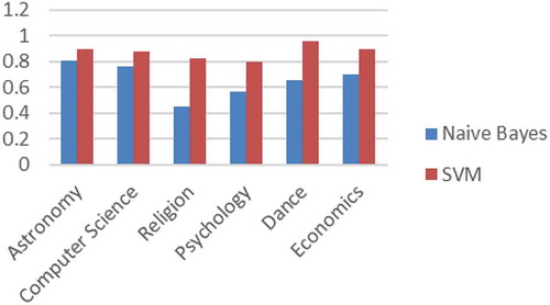
Figure 2 shows the comparison of Precision Values for Naive Bayes and SVM across the six categories. It can be observed that SVM outperforms Naive Bayes for all the categories with varying degrees of superiority. We make the following inferences from the trends.

1. SVM performs consistently well with high precision across all categories and also outperforming Naive Bayes. The latter has mixed results and varies significantly depending on the category. It performs significantly worse for Religion and Psychology in particular. We found that this is due to the overlap in the vocabulary of these two categories with various other categories, leading to misclassifications. For example, many words in articles belonging to Religion category are found in articles related to politics, terrorism, and philosophy, among others. The independence assumption of Naive Bayes is exposed as a limitation here. This problem doesn’t apply as much in highly domain-specific categories like Astronomy, which has little overlap across other subjects.

2. Because SVM also finds the optimal hyperplane (with maximal margin), the results are consistent across categories, illustrating that SVM doesn’t make assumptions about the underlying data as Naive Bayes does.

Figure 2. Precision values compared across categories for SVM & Naive Bayes.

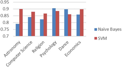
Figure 3 shows the comparison of Recall values between Naive Bayes and SVM for all the categories. Again, SVM performs better than Naive Bayes in most cases, although the gap is much closer than the Precision comparison. We also infer that Naive Bayes has very good generalization capabilities across categories and the independence assumption is helpful in that regard.

Figure 3. Recall values compared across categories for SVM & NB.

Choosing C for SVM

Linear SVM has a regularization parameter that determines whether the model will possess a hard margin (wide) or soft margin (narrow with more room for mis-predictions). Our goal initially was to extract as many articles as possible for any particular category even if the accuracy was compromised (up to an extent). We experimented with values of and determined Recall values. was chosen to obtain high Recall. Essentially, the hard margin classifier was ignored.

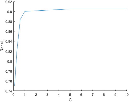
Figure 4 shows a plot indicating how Recall varies as C is changed for Astronomy. For C = 0.1, we have a value of 0.75. It increases up to 0.905 for C = 1 and after that it remains constant. Hence, any value >1 is preferable for C with Recall maximization being our goal so as to achieve completeness for that particular category with respect to Wikipedia. We observed a similar trend for other categories.

Figure 4. Recall increases with C up to 1 and then remains constant.

Conclusions

We have compared and evaluated Precision and Recall for two standard text classifiers on the full Wikipedia corpus with mostly desirable results regarding accuracy and extensibility (to different categories). However, several challenges and shortcomings must still be addressed. A better MediaWiki XML parser would produce a better document representation, giving even more accurate results without any modification to existing classifiers. Deep learning techniques like neural networks have become highly popular, and this application can be extended to them as well as other classification techniques. Another way to improve classification accuracy is taking into context the non-textual content of an article, i.e. images and other media, as part of the classification process.

Additional information

Funding

The work of the authors was supported by the Howard Hughes Medical Institute grant [HHMI-4215580].

References

- Cappabianco, F. A. M., J. P. Papa, and A. X. Falcão. 2010. Optimizing optimum-path forest classification for huge datasets. International Conference on Pattern Recognition, Istanbul, Turkey.
- Cortes, C., and V. Vapnik. 1995. Support-vector networks. Machine Learning 20 (3):273–97. doi:10.1007/BF00994018.
- Denoyer, L., and P. Gallinari. 2006. The Wikipedia XML corpus. International Workshop of the Initiative for the Evaluation of XML Retrieval, INEX 2006. Lecture Notes in Computer Science, 4518. Springer, Berlin, Heidelberg.
- Gattani, A., D. S. Lamba, N. Garera, M. Tiwari, X. Chai, S. Das, S. Subramaniam, A. Rajaraman, V. Harinarayan, and A. Doan. 2013. Entity extraction, linking, classification, and tagging for social media: A Wikipedia-based approach. Proceedings of the VLDB Endowment 6 (11). doi:10.14778/2536222.2536237.
- Joachims, T. 1998. Text categorization with support vector machines: Learning with many relevant features. European Conference on Machine Learning, Chemnitz, Germany, 137–42.
- Joshi, M. V., G. Karypis, and V. Kumar. 1998. ScalParC: A new scalable and efficient parallel classification algorithm for mining large datasets. Parallel Processing Symposium.
- Manning, C. D., P. Raghavan, and H. Schütze. 2008. Introduction to information retrieval. 1st ed., 258–69. Cambridge University Press, New York, NY, USA.
- McCallum, A., and K. Nigam. 1998. A comparison of event models for Naive Bayes text classification. Learning for Text Categorization: Papers from the 1998 AAAI Workshop, 41–48.
- Mehdi, M., C. Okolib, M. Mesgaric, F. Å. Nielsend, and A. Lanamäkie. 2017. Excavating the mother lode of human-generated text: A systematic review of research that uses the Wikipedia corpus. Information Processing & Management 53 (2) (Elsevier). doi:10.1016/j.ipm.2016.07.003.
- Murugeshan, M. S., K. Lakshmi, and S. Mukherjee. 2009. Exploiting negative categories and Wikipedia structures for document classification. International Conference On Advances in Recent Technologies in Communication and Computing, Kottayam, Kerala, India.
- Pedregosa, F., G. Varoquaux, A. Gramfort, V. Michel, B. Thirion, O. Grisel, M. Blondel, P. Prettenhofer, R. Weiss, V. Dubourg, J. Vanderplas, A. Passos, D. Cournapeau, M. Brucher, M. Perrot, and É. Duchesnay. 2011. Scikit-learn: Machine learning in python. Jmlr 12:2825–30.
- Platt, J. C. 1999. Fast training of support vector machines using sequential minimal optimization. Advances in kernel methods, 185–209. MIT Press, Cambridge, MA, USA.
- Wang, P., and C. Domeniconi. 2008. Building semantic kernels for text classification using Wikipedia. ACM SIGKDD International Conference on Knowledge Discovery and Data Mining, Platt 2009, 713–21.
- Wang, P., J. Hu, H.-J. Zeng, and Z. Chen. 2009. Using Wikipedia knowledge to improve text classification. Knowledge and Information Systems 19 (3):265–81. (Springer). doi:10.1007/s10115-008-0152-4.