Feature Selection via Pareto Multi-objective Genetic Algorithms

ABSTRACT

Feature selection, an important combinatorial optimization problem in data mining, aims to find a reduced subset of features of high quality in a dataset. Different categories of importance measures can be used to estimate the quality of a feature subset. Since each measure provides a distinct perspective of data and of which are their important features, in this article we investigate the simultaneous optimization of importance measures from different categories using multi-objective genetic algorithms grounded in the Pareto theory. An extensive experimental evaluation of the proposed method is presented, including an analysis of the performance of predictive models built using the selected subsets of features. The results show the competitiveness of the method in comparison with six feature selection algorithms. As an additional contribution, we conducted a pioneer, rigorous, and replicable systematic review on related work. As a result, a summary of 93 related papers strengthens features of our method.

Introduction

Classification is a well-known data mining task, where one seeks to build models that extract patterns from a dataset, which can be afterwards used for predicting the label of new data (Han and Kamber 2011). In general, data for classification problems are labeled, containing one or more classes for each input instance. The objective is to obtain a model that relates the input features of the data points (instances) to their output labels. In this article, we deal with single-label classification problems, where each data point has a unique output label.

The presence of irrelevant and/or redundant features in a dataset, associated to the effects from the “curse of dimensionality,” can impair the performance of classification models built using such data. Furthermore, the computational cost in obtaining these models is usually higher and data with many features can also be considered more complex to understand (Guyon and Elisseeff 2003). Thus, removing non-important features from a dataset is a significant goal to achieve.

Feature Selection (FS) methods have been deeply studied in the literature to tackle these problems (Liu and Motoda 2007). FS can be viewed as a search for subsets of important features in a dataset and is usually considered as a pre-processing step in the data mining process. Each feature subset is a potential state in the search space, i.e., a possible solution for the search problem. The evaluation of the different states can usually be performed by using one or more importance measures, which estimate the quality of the feature subsets based on a specific purpose, such as for building better classification models.

Filter importance measures are based on information extracted from data only, addressing different aspects useful for data classification. On the other hand, importance measures applied according to the wrapper approach use a classification algorithm to estimate the quality of the feature subsets. Alternatively, the embedded approach selects features during classifier training. In contrast to wrapper and embedded FS, the filter approach is less biased toward a specific classification algorithm and usually can be performed at a lower computational cost. Moreover, the dataset is pre-processed only once and can be used as input to different classification algorithms. In this article we adopt the filter approach.

The search process related to FS can be solved by using heuristic methods such as Genetic Algorithms (GA) (Yang and Honavar 1998). In GA, feature subsets are often encoded as chromosomes, in which each gene represents the selection of a specific feature from the dataset, while importance measures are optimized as fitness functions. The standard Single-objective Genetic Algorithm (SOGA) focuses on one importance measure only, while Multi-objective Genetic Algorithms (MOGA) consider two or more importance measures simultaneously. MOGA provides support to the simultaneous optimization of potentially conflicting functions during the search for feature subsets. This fact is useful to accommodate relevant, but accidentally contradictory functions in data mining, such as classification accuracy and simplicity (Freitas 2004).

One of the most common approaches to dealing with such scenario is by using the Pareto dominance theory, as done by algorithms such as the usual Non-dominated Sorting Genetic Algorithm (NSGA-II) (Deb et al. 2000), where multiple objectives can be analyzed without any weighting.

The purpose of this study is to extend and integrate our previous pieces of work on the topic (Spolaôr, Lorena, and Lee 2011a, 2010b). Besides a more complete description of the developed MOGA and a uniform analysis of the most relevant experimental results, this article considers a wider range of datasets and importance measures than most of the related publications. It should be emphasized that, although the focused method currently supports the optimization of six feature importance measures and their combinations, we opted to present here a deeper evaluation of some combinations of pairs of simple measures, highlighted as most promising in our previous work and flexible enough to deal with both quantitative and qualitative features.

To gather evidence on related work, we conducted a Systematic Review (SR) to identify the use of MOGA for FS in the literature. According to the SR, few papers select features by using filter importance measures in MOGA. Moreover, many of these papers investigate a few labeled datasets, from specific domains, and study only two importance measures. This panorama from related work strengthens features of the method focused in this article, such as the flexibility to explore different filter measures in experimental evaluations with several datasets. The developed method can also be adapted to work on both labeled and unlabeled datasets, although we currently considered a supervised scenario only, for better uniformness.

This article is organized as follows: Section 2 describes basic concepts related to FS. Section 3 presents the MOGA method proposed for FS. Section 4 summarizes related work found by conducting the systematic literature review method (Kitchenham and Charters 2007). Section 5 describes the experimental setup, whose results are discussed in Section 6. Section 7 concludes this article.

Feature selection

Machine Learning (ML) techniques solve classification problems by extracting patterns from datasets with known instances, in an induction process. A dataset is composed of data points , in which each has features describing properties and characteristics of the data point. A usual representation of the data submitted to ML algorithms is the feature-value format. As exemplified at Table 1, in this format each column corresponds to a feature, with discrete (qualitative) or numeric (quantitative) values, and each row is an instance of the dataset. In classification problems, each data point is also accompanied by a discrete label , as presented at Table 1. The objective of the learning algorithm in such scenario is to obtain a model able to predict the labels of unknown instances.

Table 1. Data represented according to the feature-value format.

Features				Label
		…
		…
		…

Feature selection provides support to identify a subset of important features in a dataset. As a result, a new and smaller dataset, composed of instances described by a lower number of features, is specified. Using the pre-processed dataset as input to an ML technique can lead to the obtainment of similar or better models than using all input features, with a reduced training cost. A better understanding of data is also achieved, by the identification of the most important characteristics of the data points. In high dimensional domains, such as gene expression analysis, another benefit is a reduction of effects associated to the curse of dimensionality.

Feature subset search

FS can be viewed as a search process for a high quality feature subset that maximizes or minimizes one or more importance measures. Given a dataset with features, each combination of features is a possible solution or state in this search. As a result, the search space is composed of all possible combinations of the features, i.e., all feature subsets regarding the features. Searching for the best subset of features involves moving through the states in this space according to four parameters: state evaluation criteria, search direction, search strategy and stop criterion.

Regarding the evaluation of the states, there are criteria for the individual or joint evaluation of the features in a subset. When considering the importance of each feature individually, a ranking of the features according to the score calculated by a measure is usually obtained. By using a threshold on the feature scores or on the number of features to be chosen, a subset of features can be selected. A disadvantage of feature ranking is that redundant features are usually ranked close to each other and tend to be jointly selected (Hall 2000). Therefore, redundant features can remain on the dataset. In this work, we used mainly feature importance measures that perform a joint evaluation of the features contained in a given subset. In such case, the features in the subset are evaluated regarding their joint importance.

The evaluation criteria for features subsets can also be categorized according to their interaction to an induction (classification) algorithm (Kohavi and John 1997). In the embedded approach the FS is performed internally by the induction algorithm during its training. The wrapper approach uses an induction algorithm as a black-box to evaluate candidate feature subsets in the search process. The filter approach, employed in this work, considers intrinsic properties of data, and does not involve any interaction with a particular induction algorithm.

The search directions define the sequence of states accessed during the search. The main search directions are forward, backward, and random (Liu and Motoda 1998). In forward direction, search begins from an empty feature subset and features are gradually added until a stop criterion is reached. Backward search does the opposite, beginning with all features and gradually discarding features from this set. In random direction there is no specific starting point. Genetic Algorithms fall into the last category, due to their stochastic nature and exploration of multiple solutions.

The search strategies can be complete, heuristic, or non-deterministic (Liu and Yu 2002). In complete search, all optimal states are identified. Although this search may be non exhaustive, as in Branch & Bound algorithms, it is usually costly to perform. Heuristic search is oriented by a specific knowledge of the problem to find potential good states at each step. This strategy is useful for FS in large datasets to save computational resources. Finally, non-deterministic search travels the search space randomly. GA use heuristic functions in a non-deterministic search.

The search process in FS can be stopped when a given number of features is selected or if no improvement can be achieved by adding or removing features from a subset. Another possible criterion is when a maximum number of iterations of the search is reached.

Categories of feature importance measures

A feature is relevant if its removal implies in the deterioration of the learning performance calculated when the feature was included in the data. Liu and Motoda describe a taxonomy of five categories of feature importance measures: consistency, dependency, distance, information, and precision (Liu and Motoda 1998). These categories can be briefly described as:

Consistency

Involves identifying a subset of features which allows to build a consistent hypothesis from data. For labeled data, consistency is related to the low occurrence of examples with similar values in the features, but distinct labels.

Dependency

They are also known as correlation or association measures. These measures consider, for example, the ability to predict the value of a feature from the value of another feature.

Distance

Also known as separability or discrimination measures. Important features according to these measures are those which allow a better discrimination of the concepts or classes present on data.

Information

Determine the information gain in using one or more features, that is, the difference between the a priori and the a posteriori uncertainty associated to the inclusion or elimination of features.

Precision

Considers the performance achieved by a classification model when using a particular subset of features. Therefore, this type of measure involves the interaction between FS and an induction algorithm.

Except from precision, all other categories provide measures that are based on different aspects from data. Since precision measures need to interact with an induction algorithm, they are not employed for filter FS and, as a consequence, they are not considered in this article. We chose measures from all the categories, except precision, to be combined in an MOGA. They are described in Section 3.1.

Feature selection via multi-objective genetic algorithm

As presented in Section 2, FS can be stated as a search for subsets of features optimizing some feature importance criterion. Genetic Algorithms (GA) are search and optimization techniques based on principles of Natural Evolution and Genetics frequently used in FS. They evolve a population of possible solutions to the problem by the application of a proper selection mechanism and of genetic operators to generate new solutions. Their usual application in FS consists in searching for a feature subset optimizing a given feature importance measure. The most commonly used representation for the individuals consists in a binary string with bits, one for each feature in the original dataset. A value of in gene indicates the selection of feature , while a value of implies that the feature is not selected. The importance measure is employed as a fitness function, i.e., in the evaluation of the feature subsets encoded in the individuals.

Nonetheless, it may be interesting to consider multiple aspects when evaluating the quality of a feature subset. Multi-objective Genetic Algorithms (MOGA) adapts the standard GA to the consideration of multiple objectives. Therefore, they can then be employed in the search for subsets of features which optimize multiple feature importance measures simultaneously (Zaharie et al. 2007).

As discussed in Section 2.2, there are different categories of importance measures that can be considered when evaluating a feature subset in FS. For each of the categories, there are also various measures that can be defined, looking at distinct aspects from data. In this work we use an MOGA to perform the search for subsets of features optimizing a combination of feature importance measures from different categories. The choice of measures from different categories is motivated by the possibility to explore eventual complementarities between them. We only consider measures that can be captured from the datasets, that is, feature importance measures that are representatives from the consistency, dependency, distance and information categories. Therefore, the method can be characterized as a filter approach for FS.

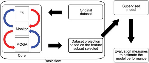
Figure 1 shows the modules that compose the core of the method implemented in this study. Both Monitor and Multi-objective Genetic Algorithm (MOGA) modules used are the same available in the Platform and Programming Language Independent Interface for Search Algorithms (PISA) framework (Bleuler et al. 2003). In particular, we chose the Non-dominated Sorting Genetic Algorithm (NSGA-II), which is a usual MOGA with concepts based on the Pareto theory for multi-objective optimization, in the MOGA module. By default, all objectives in PISA must be minimized. Moreover, the values of the objectives cannot be negative. Therefore, some feature importance measures had to be adapted accordingly. The Feature Selection (FS) module was adapted from a PISA module related to the Knapsack optimization problem.

Figure 1. Modules of the method developed in this work and their interactions. In particular, the monitor module manages the remaining components, which in turn perform feature selection and multi-objective optimization by a genetic algorithm.

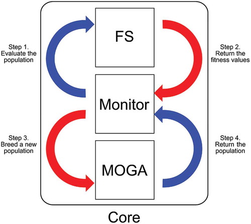
The modules interact in a systematic way during the optimization process. Given an initial population of the GA, composed of binary strings representing distinct features subsets, the Monitor module starts the FS module to evaluate the subsets of features encoded in the current population according to a given combination of importance measures. Afterwards, the Monitor manages a loop composed of two main procedures: (1) MOGA applies the selection and genetic operators, generating new individuals; (2) the FS module evaluates the current population using the importance measures being combined. The loop ends when a stop condition is reached, which was set to a maximum number of iterations of the MOGA in our experiments. The selection mechanism employed is the binary tournament and the genetic operators used were one-point crossover and bit-flip mutation. The remaining MOGA parameter values are described and justified in Section 5.2.

Given a dataset represented in a feature-value format as input, the output of the method is a reduced version of the dataset that is described by the features selected in the optimization process. NSGA-II gives several solutions, which represent different trade-offs in the optimization of the objectives, in accordance to the Pareto-based multi-objective optimization theory. We chose a unique feature subset using the Compromise Programming technique (Zeleny 1973). This simple technique consists of choosing the solution with the lowest distance to a reference point. For minimization, this point corresponds to a vector composed of the lowest values of the objective functions achieved within all MOGA solutions.

In what follows, the importance measures implemented in the FS module are described.

Importance measures considered

In order to explore distinct aspects from data, we chose importance measures from each one of the following categories: consistency, dependency, distance, and information.

For consistency evaluation, we used the Inconsistent Example Pairs (IP) (Arauzo-Azofra, Benitez, and Castro 2008) measure. This measure identifies the inconsistency rate of a dataset based on the number of inconsistent pairs of instances divided by the total number of pairs of instances. An inconsistent pair is characterized by presenting similar values for their features, while their class labels are different. Quantitative features must be discretized before calculating this rate. The higher the rate, the more inconsistent the feature subset is. In this work, the same discretization procedure considered in (Arauzo-Azofra, Benitez, and Castro 2008) is employed before applying IP.

Concerning dependency, the Attribute-class Correlation (AC) is used, as defined by Eq. (1). In this equation, will be if the feature is selected and otherwise; if the instances and have distinct labels or otherwise; represents the feature value from ; and denotes the module function. This measure highlights features that have more distinct values for instances of different classes. AC can also be used for qualitative features, by replacing the difference in the module (Eq. (1)) by the overlap function (Wilson and Martinez 1997), in which features with the same value show a difference of 1, while equal feature values have null difference.

(1)

Another dependency measure used was the Intra-Correlation (IC), defined by Eq. (2) (Wang and Huang 2009). It considers the Pearson correlation between the feature vectors in a subset ( corresponds to the column vector of the feature). It normalizes the global correlation of a feature subset, using as the number of 2-combinations of features, and as the number of features of this subset.

(2)

The Inter-Class Distance measure—IE—(Zaharie et al. 2007) estimates the separability between classes in a dataset when using a given subset of features. Eq. (3) defines IE, where is the central instance (centroid) of the dataset, denotes the Euclidean distance or the overlap function for qualitative features, is the number of classes and and represent, respectively, the centroid and the number of instances in the class .

(3)

The Laplacian Score—LS—(He, Cai, and Niyogi 2005) is also a distance based importance measure and takes into account the fact that instances related to the same concept tend to be close in the input space. In classification, for instance, this behavior can be observed among instances of the same label, highlighting the importance of modeling their local structure. LS builds a nearest neighbor graph, in which each node corresponds to a distinct instance and its nearest instances are connected to it. Eq. (4) defines the LS measure, with and . This formula includes the matrices and , where , in which extracts the diagonal matrix and is the weight matrix of the graph edges, while is called the Laplacian Graph.

(4)

In the information category, we considered the Representation Entropy—RE—(Mitra, Murthy, and Pal 2002) measure, defined by Eq. (5). The eigenvalues , calculated by the GNU Scientific Library, are extracted from a covariance matrix of the feature values of order . If all eigenvalues are equal, the information is distributed uniformly in the data and there is low redundancy. On the other hand, if only an eigenvalue is different from , then all information could be represented by a single feature.

(5)

All measures, except from LS, allow to evaluate a given subset of features jointly. For such, reduced versions of the dataset are built using the subset of features and the measures can then be calculated. On the other hand, LS evaluates each feature individually. We employed the average of the LS values of all features in a subset as a joint measure, such that all chosen measures perform joint feature evaluation.

Another important observation is that the PISA platform, used in the MOGA implementation, supports only the minimization of objective functions. This demanded a transformation of the maximization problems related to the AC, IE, and RE measures into equivalent minimization problems. To do so, for each measure, we subtract the corresponding objective values from the highest value reachable in the measure. In addition, the MOGA module assumes that all objectives have non-negative values, but the AC measure can reach negative values. Then, the AC original range of objective values was transformed into a range composed of positive values only, by summing the lowest value possible for AC.

Table 2 gives an overview of the main characteristics of each of the importance measures mentioned in this article. This table shows the category of the measures and the feature type they are able to deal with (where QL stands for qualitative values and QT stands for quantitative values).

Table 2. Importance measures employed. These measures are associated with distinct categories and can deal with Quantitative (QT) and Qualitative (QL) feature values.

Importance measure	Category	Feature Type
Inconsistent Example Pairs (IP)	Consistency	QL+QT
Attribute-class Correlation (AC)	Dependency	QL+QT
Intra-Correlation (IC)	Dependency	QT
Inter-Class Distance (IE)	Distance	QL+QT
Laplacian Score (LS)	Distance	QT
Representation Entropy (RE)	Information	QT

Related work found by the systematic review method

A Systematic Review (SR) was carried out to identify related work on the use of MOGA in FS (Spolaôr, Lorena, and Lee 2010a). The SR method is composed of three main steps: planning, conducting, and reporting (Kitchenham and Charters 2007). The planning step specifies the research questions that must be answered and creates a search protocol. The activities that integrate this protocol are carried out in the next step in order to identify a set of publications able to answer the research questions. The last step involves reporting the results in different ways, such as technical reports, PhD thesis, and papers.

The SR was performed by us in June 2010 (Spolaôr, Lorena, and Lee 2010a) and updated in January 2015 to answer research questions such as “What are the applications of MOGA in FS?”. A total of 93 publications on MOGA applications were found, from which 21 use the MOGA according to the filter approach. The 21 related studies are cited in the supplementary material available at https://db.tt/3iGgSTc5 and considered in what follows.

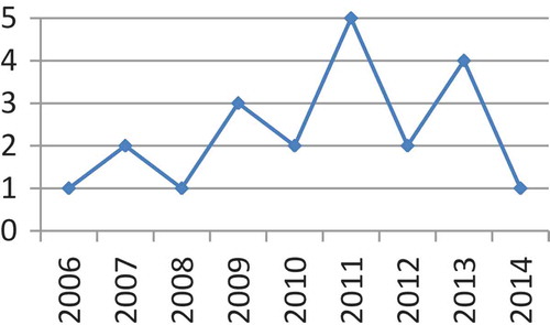
In this work, we address specific gaps of the literature, such as the use of filter importance measures from different categories and the application to different scenarios and data. Figure 2 shows how previous work on MOGA application for filter feature selection distribute along the years. This relatively recent research topic has been considered in publications at least once a year from 2006.

Figure 2. Frequency of related papers per year of publication.

Most of the related papers is devoted to FS applied to data from a specific domain, such as bioinformatics, medicine, economics, computer networks, signal, and image analysis. The exceptions are (Nahook and Eftekhari 2013; Santana, Silva, and Canuto 2009; Saroj 2014; Xue et al. 2013) and our previous work on the topic (Spolaôr, Lorena, and Lee 2011a, 2010b), which consider datasets from various domains.

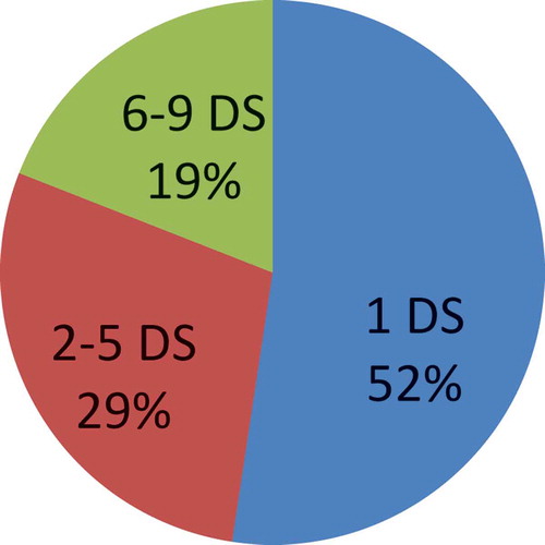
Figure 3 shows that most of the related papers () consider at most 5 datasets. It should be emphasized that this work uses more datasets than all MOGA applications for filter FS: 12—Section 5.1.

Figure 3. Percentage of related papers using specific numbers of datasets.

The NSGA-II Pareto-based MOGA is also the most used algorithm in related work, as exemplified in (Saroj 2014; Spolaôr, Lorena, and Lee 2011a; Xue et al. 2013; Zaharie et al. 2007). There are also papers employing a weighted sum of objectives in a standard GA. Nevertheless, in such approach one has to properly tune the weights given to each objective.

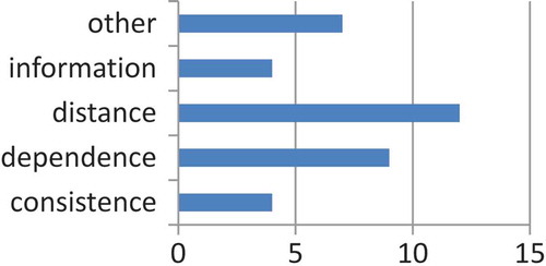
Figure 4 summarizes the categories of the feature importance measures by taking into account their frequency of use in related work on the filter approach. Although all categories are shown, only seven papers consider the combination of feature importance measures from distinct categories. A few pieces of work use importance measures which consider characteristics and properties of the application they deal with. Four of the related publications also consider the cardinality of the feature subset as an objective to be explicitly minimized.

Figure 4. Categories of feature importance measures used in related work.

Concerning our previous work, we compared 10 MOGA for filter FS in 5 labeled datasets in (Spolaôr, Lorena, and Lee 2010b). Only pairs of feature importance measures were considered, since previous experiments pointed disadvantages in the optimization of more measures. The main contribution was to highlight MOGA which optimize the simple inter-class distance measure (IE), motivating further investigations.

Four MOGA based on IE in combination to other measures were evaluated in nine labeled datasets in (Spolaôr, Lorena, and Lee 2011a). Two popular filter feature selection algorithms, named Correlation-based Feature Subset Selection (Hall 1999) (CFS) and Consistency Subset Evaluation Evaluation (Liu and Setiono 1996) (CSE), as well as five SOGA (Single-Objective Genetic Algorithms) based on each criterion individually were used for comparison. The best results were obtained with MOGA IE+AC, CFS, and CSE, which were competitive according to a statistical test at the significance level .

We employed the proposed MOGA in 12 labeled and 7 unlabeled datasets in (Spolaôr, Lorena, and Lee 2011b). The feature importance measures IE, AC, and IP were modified, aggregating the capability to address qualitative data. In addition, MOGA based on IC, RE and LS measures were used to perform FS in unlabeled data. The numerical results against models built using all features were promising, highlighting the MOGA IE+AC and IE+IP in data with both quantitative and qualitative features, respectively.

In this article, we extend such work by including a more extensive description of the MOGA proposed and a wider and more uniform experimental evaluation of the most relevant results, based on visual and numerical comparison procedures, as well as datasets with quantitative and qualitative features.

Experimental design

In order to evaluate the effectiveness of the feature subsets identified by the MOGA, we generated classification models from data described by the subsets and verified the performance achieved by them compared to the one achieved by models using all features. The same procedure was adopted for other FS techniques used as baseline. Figure 5 summarizes this experimental flow for FS. Starting from a dataset, FS is applied and the result is a reduced version of the input dataset, described by less features.

Figure 5. Experimental flow adopted in the evaluation of FS.

When inducing the classification models, four classification algorithms from different paradigms—the decision tree J48 (Witten and Frank 2011), Support Vector Machine (SVM) (Scholkopf and Smola 2001), Naive Bayes (NB) (Mccallum and Nigam 1998), and -Nearest Neighbor (NN) (Aha and Kibler 1991)—from the Weka tool (Witten and Frank 2011): data were applied, in order to reduce the influence of a specific algorithm on the results and to improve the experimental evaluation generality. Their parameters were kept with default values.

In addition, we also recorded the percentage of reduction in the number of features achieved by the FS algorithms. FS algorithms that are able to reduce more the number of features, while still maintaining the core patterns of the dataset can be considered better. The comparison of models built using the pre-processed and original datasets allow us to identify whether the main predictive characteristics of a dataset were maintained.

The datasets and algorithms used in the experiments are presented next.

Datasets

We chose 12 datasets from the UCI repository (Asuncion and Newman 2007; Bache and Lichman 2013), commonly employed in relate work (Spolaôr, Lorena, and Lee 2011a, 2010a): Australian (A), Crx (C), Dermatology (D), German (G), Ionosphere (I), Lung cancer (L), Promoter (P), Sonar (S), Soybean small (Y), Vehicle (V)—supported by the Turing Institute in Glasgow, Wisconsin Breast cancer (B), and Wine (W). Table 3 summarizes the relevant information for each dataset, including their number of instances , total number of features , number of quantitative features (QT), number of qualitative features (QL), number of classes , and percentage of the Majority class Error (ME), which corresponds to the error rate obtained by classifying all data in the majority class.

Table 3. Summary of the datasets used in this study: Australian (A), Crx (C), Dermatology (D), German (G), Ionosphere (I), Lung cancer (L), Promoter (P), Sonar (S), Soybean small (Y), Vehicle (V), Wisconsin Breast cancer (B) and Wine (W).!

	A	C	D	G	I	L	P	S	Y	V	B	W
	690	653	358	1000	351	32	106	208	47	846	569	178
	14	15	34	20	34	56	57	60	35	18	30	13
QT	14	6	34	7	34	56	0	60	35	18	30	13
QL	0	9	0	13	0	0	57	0	0	0	0	0
	2	2	6	2	2	3	2	2	4	4	2	3
ME (%)	45	45	69	30	36	59	50	47	64	74	37	60

All datasets were divided according to the -fold stratified cross-validation strategy, resulting in pairs of training and test sets which preserve the class distribution of the original dataset (Han and Kamber 2011). Training sets are used in FS and to build classification models, while test sets are used during the evaluation of such models.

Baseline algorithms

Three groups of algorithms were used for comparison against the MOGA. The first group consists of SOGA algorithms, each one optimizing an importance measure from Section 3.1 individually (single-objective) according to the filter approach.

Another group is composed of four SOGA algorithms following a wrapper approach, optimizing the error rate achieved by a particular classifier. We use four popular classification algorithms from different learning paradigms in such evaluation: (1) the decision tree J48, (2) support vector machine, (3) Naive Bayes, and (4) -Nearest Neighbor. In the last step of the experimental flow (Figure 5), each feature subset produced by the wrappers was evaluated using the same classification algorithm employed during FS. Therefore, we expect that the results of these SOGA will be optimized and better for each of their respective classification algorithms.

All SOGA algorithms use the same encoding, selection mechanism, genetic operators, and stop condition as the MOGA. This was done to better analyze whether the multi-objective optimization of feature importance measures overcomes the optimization of each isolate measure. For MOGA we used the NSGA-II implementation available in the PISA with the following parameters: , , , , , . The parameters , , and correspond, respectively, to the population size and the number of parents and children after reproduction. These parameter values were defined based on population sizes usually employed in the related work described in Section 4.

The last algorithm for comparison was an ensemble of feature ranking algorithms (EH) (Prati 2012), composed of three popular importance filter measures from literature: Information Gain (IG) (Liu and Shum 2003), Symmetrical Uncertainty (SU) (Press et al. 1992), and the measure inherent to the ReliefF algorithm (RF) (Robnik-Sikonja and Kononenko 2003). EH can also be regarded as an alternative to combine distinct importance measures. The aggregation was performed according to the Borda approach (Dwork et al. 2001), in which each feature has a general rank based on a weighted sum of the rankings assumed by this feature for each of the FS algorithms aggregated. We then select the best features, i.e., 50% of the best features in the general ranking. This threshold was chosen due to its use in previous studies (Spolaôr, Lorena, and Lee 2011a) and its relevance in a supervised comparison procedure (Lee, Monard, and Wu 2006). For instance, we consider that the performance of a FS algorithm is very good if it is able to reduce 50% or more of the features, while maintaining or improving the accuracy value observed for all features. An advantage of EH over other ensemble methods is that it is flexible to work with different FS algorithms.

Evaluation procedures

As already discussed, the main comparison procedure adopted was to build classification models using the feature subsets identified by each FS algorithm.

In addition, we employed in this article a comparison model based on a trade-off between the reduction of the size of a feature subset and of the error rate (complement of accuracy for learning performance) achieved by the classifiers. It is important to emphasize this trade-off, as reaching good learning performance only is not the unique goal for some applications. In some cases, feature subset size reduction can be also important, for example, to build faster and less complex classifiers (Guyon and Elisseeff 2003). Decision trees (Witten and Frank 2011) are an example of learning algorithm that can yield simpler classifiers when some non-important features are discarded.

The comparison model, proposed in (Lee, Monard, and Wu 2006), plots the error rate achieved ( axis) by using a percentage of the features ( axis). Each classifier will originate one of such graph for a given dataset. Figure 6 shows an example of this trade-off graph.

Figure 6. Comparison procedure based on error rate (axis X) and size of feature subsets (axis Y) (Lee, Monard, and Wu 2006).

In this graph, EF stands for the Error without Feature selection, i.e., the error rate of the model built using all features. ME’ is equal to the majority class error (ME) if this value is lower than 0.5, or equal to 0.5 otherwise. MR is the average of EF and ME’. A good FS algorithm should reduce the datasets, while still building classification models of good performance. Therefore, some regions of quality are defined in Figure 6, based on thresholds defined on both axes. If the error rate reduces and is lower than EF, the performance is considered excellent. A very good performance is verified when the classification error is acceptable, while a sharp reduction of 50% or more of the features is obtained. A good performance is achieved when the error rate is maintained acceptable, but more modest reductions in the number of features are verified. If the classification error is above the ME’ value, the performance is considered very poor, despite having reductions in the number of features. On the other hand, if the classification error approaches ME’ and more than 50% of the features were disregarded, the performance is poor, since this probably corresponds to the case where the most important features were those eliminated.

Each classifier built after using an FS algorithm is plotted in the graph as a point and categorized according to the region it falls within. This procedure was extended in this article to also include the result of a statistical test comparing each MOGA against the two related SOGA, i.e., the two SOGA optimizing the importance measures taken into account by the MOGA. This test considers the confidence interval based on the Student’s t distribution at the significance level .

For MOGA results that are statistically better than the SOGA ones, the correspondent point is a blue filled square, while the green hollow square was used to symbolize MOGA results statistically worse than the SOGA ones. A red triangle denotes the absence of statistical difference. Finally, the SOGA results are represented by blue hollow circles.

Experimental results

We show and analyze here the results of two combinations of measures representing different categories (Section 2.2): IE+AC and IE+IP. The choice to deepen the analysis on these MOGA is based on results from our previous work, which were summarized in Section 4, as well as the support provided by the corresponding measures to deal with both quantitative and qualitative features—Table 2. In particular, IE+AC was the best MOGA according to experimental evaluations conducted in datasets with quantitative features, whereas IE+IP presented the same behavior in analysis regarding datasets with qualitative features. It should be emphasized that the IP measure discretizes the data before evaluating quantitative features (Section 3.1), which could have hindered its experimental performance.

One can also note that these MOGA combine measures from different categories that use class information as an attempt to support feature evaluation. Finally, it is important to emphasize that optimizing three or more importance measures led to higher computational cost with small gains in classification performance, as pointed in (Spolaôr, Lorena, and Lee 2011a).

Due to the stochastic nature of genetic algorithms, they were executed five times for each training dataset. This strategy results in five feature subsets per algorithm and, consequently, five reduced versions of the dataset. Therefore, five classification models are also induced according to -fold stratified cross-validation, and the results for GA shown correspond to the average from 10 trainings sets*5 runs = 50 results.

Reduction in the number of features

Table 4 shows the average and the corresponding standard deviation of the Percentage of Reduction (PR) in the number of features obtained by each FS algorithm, including the baselines. Cells with average PR greater than 50% are highlighted in bold. In this table, AC, IE, and IP rows correspond to the single optimization of these measures by SOGA. WJ, WS, WB, and WN are the wrapper algorithms employing the J48 (Decision Tree), SVM, Naive Bayes, and Nearest Neighbor classifiers, respectively. EH, which stands for the ensemble FS, always removes 50% of the features and is not shown.

Table 4. Percentage of Reduction (PR) in the number of features for each dataset. Cells with average PR greater than 50% are highlighted in bold.

PR	A	C	D	G
IE+AC	57.14(0.45)	60.00(0.00)	22.94(1.46)	89.90(0.14)
IE+IP	0.00(0.00)	9.07(0.69)	0.00(0.00)	8.10(1.21)
AC	92.86(0.00)	93.33(0.00)	97.06(0.00)	95.00(0.00)
IE	4.86(0.68)	50.67(0.49)	1.47(0.71)	53.60(0.81)
IP	92.86(0.00)	90.67(1.98)	65.41(1.13)	95.00(0.00)
WJ	57.29(1.25)	56.13(1.49)	70.76(1.41)	59.50(1.31)
WS	88.00(1.24)	86.53(0.77)	60.88(1.88)	40.20(1.86)
WB	42.86(1.41)	54.40(1.17)	46.76(2.62)	43.30(1.64)
WN	68.71(1.18)	73.07(1.34)	51.12(2.66)	77.10(2.60)
PR	I	L	P	S
IE+AC	32.59(1.35)	35.36(1.96)	24.60(2.63)	56.47(2.46)
IE+IP	1.41(0.50)	1.04(0.73)	11.68(2.22)	5.73(1.70)
AC	96.65(0.45)	96.96(1.22)	97.16(1.03)	92.43(3.89)
IE	5.47(0.97)	9.57(1.88)	70.14(3.04)	14.77(2.67)
IP	70.47(0.90)	81.04(2.18)	85.26(0.90)	83.77(1.14)
WJ	77.88(2.32)	85.50(3.84)	80.95(3.25)	68.23(4.32)
WS	56.41(2.42)	73.50(3.73)	60.35(3.47)	58.27(4.24)
WB	67.53(1.94)	71.96(3.07)	61.30(4.28)	66.43(4.28)
WN	69.06(2.48)	71.43(5.14)	51.51(4.45)	54.13(3.92)
PR	Y	V	B	W
IE+AC	59.60(0.50)	7.44(0.72)	69.40(0.44)	37.69(0.95)
IE+IP	20.40(1.65)	0.00(0.00)	0.00(0.00)	0.00(0.00)
AC	97.14(0.00)	94.44(0.00)	96.67(0.00)	92.31(0.00)
IE	33.83(1.25)	0.22(0.20)	20.27(1.94)	8.00(1.01)
IP	85.66(1.61)	94.44(0.00)	70.80(0.89)	59.54(0.44)
WJ	86.97(1.59)	37.11(1.75)	76.13(1.93)	70.15(0.63)
WS	83.54(1.57)	20.56(1.28)	47.87(2.11)	40.31(1.29)
WB	87.31(1.59)	47.78(1.32)	67.33(2.11)	43.85(2.17)
WN	87.37(2.12)	43.44(1.40)	53.00(2.21)	48.77(1.02)

Some baseline algorithms have lead to high reductions in PR, mainly the wrappers (although their standard deviation is higher). This was also verified for the SOGA IP and AC. IE was more conservative and maintained more features. This was also reflected in the results of the MOGA IE+AC and IE+IP, both related to IE, despite of AC and IP having lead to large reductions. Moreover, IE+AC was able to obtain reductions higher than 50% in various datasets. Therefore, one measure complemented each other regarding PR.

Predictive performance

Tables 5 and 6 present the average accuracies of the predictive models built in this work. Specifically, Table 5 shows the results of the J48 and SVM classifiers, while Table 6 shows the results of the NB and NN classifiers. Those cells of FS algorithms which obtained PR (Table 4) greater than 50% are highlighted by an asterisk. In addition, the cells in italics indicate models with accuracy worse or equal to the Majority Class Error. Figure 7 summarizes these results by taking into account the area of a polygon specific for each classification method and FS algorithm. Each polygon in turn is composed of 12 axes, in which each axis represents the average accuracy achieved by the correspondent classifier and FS strategy in a particular dataset.

Table 5. Performance of J48 and SVM models for each dataset. Cells regarding FS algorithms that obtained PR (Table 4) greater than 50% are highlighted by an asterisk (*). Cells in italics indicate models with accuracy worse or equal to the Majority Class Error.

J48	A	C	D	G
IE+AC	85.36(2.57)*	76.41(5.84)*	91.14(4.64)	70.20(1.41)*
IE+IP	83.48(3.01)	85.33(3.82)	93.28(4.99)	72.32(3.59)
AC	67.68(4.14)*	68.31(5.16)*	31.00(4.03)*	70.20(0.76)*
IE	84.06(3.08)	74.75(3.34)*	93.67(4.85)	71.18(4.23)*
IP	54.93(2.31)*	59.92(11.6)*	91.93(5.84)*	70.00(0.00)*
WJ	84.00(3.48)*	85.18(4.66)*	94.36(2.62)*	72.82(4.01)*
EH	82.46(4.99)*	81.78(7.75)*	91.88(3.64)*	73.30(3.23)*
EF	83.48(3.15)	85.30(3.62)	93.28(5.20)	71.10(3.84)
J48	I	L	P	S
IE+AC	90.84(5.75)	51.00(29.19)	81.82(11.42)	81.18(8.97)*
IE+IP	90.89(5.12)	45.67(33.26)	82.91(11.66)	69.03(8.01)
AC	75.42(6.43)*	46.67(22.08)*	71.09(10.44)*	65.51(8.88)*
IE	91.00(5.16)	47.00(32.02)	84.85(12.76)*	72.41(8.37)
IP	88.70(6.03)*	51.00(28.65)*	67.18(14.28)*	69.72(10.37)*
WJ	90.77(5.30)*	36.67(20.96)*	80.49(11.08)*	75.57(7.00)*
EH	88.89(4.35)*	44.17(31.93)*	79.45(11.28)*	75.50(7.19)*
EF	90.89(5.34)	41.67(36.00)	82.91(12.17)	70.21(9.81)
J48	Y	V	B	W
IE+AC	97.50(7.58)*	72.54(4.46)	93.21(3.12)*	93.24(4.95)
IE+IP	97.50(7.58)	74.00(5.08)	94.90(2.81)	92.12(6.28)
AC	41.50(13.75)*	53.67(4.43)*	91.74(3.82)*	70.26(10.56)*
IE	97.50(7.58)	74.00(5.02)	94.62(2.83)	91.90(6.29)
IP	98.80(4.80)*	52.35(5.16)*	93.70(3.40)*	91.56(6.67)*
WJ	99.60(2.83)*	71.42(4.24)	93.46(3.22)*	93.12(4.16)*
EH	95.50(9.56)*	67.48(4.24)*	92.43(4.71)*	94.38(6.48)*
EF	97.50(7.91)	74.00(5.30)	94.90(2.93)	92.12(6.55)
SVM	A	C	D	G
IE+AC	85.51(4.58)*	71.83(4.88)*	95.41(1.94)	70.00(0.00)*
IE+IP	85.51(4.58)	85.85(4.13)	96.37(1.81)	75.44(2.90)
AC	56.38(1.66)*	55.44(1.88)*	31.02(1.13)*	70.00(0.00)*
IE	85.51(4.58)	71.83(6.34)*	96.43(1.80)	73.60(2.83)*
IP	54.93(2.31)*	59.18(11.80)*	94.29(4.10)*	70.00(0.00)*
WS	85.51(4.58)*	86.19(4.31)*	97.26(2.08)*	75.04(2.86)
EH	83.33(5.48)*	79.64(10.39)*	93.57(3.73)*	74.20(1.55)*
EF	85.51(4.78)	85.91(4.44)	96.37(1.89)	75.80(3.12)
SVM	I	L	P	S
IE+AC	85.92(4.65)	51.83(18.08)	83.71(10.34)	74.38(7.90)*
IE+IP	88.02(4.45)	45.50(16.43)	86.89(11.16)	76.02(5.54)
AC	64.79(4.65)*	47.33(20.02)*	71.95(10.04)*	64.18(9.28)*
IE	88.08(4.40)	48.67(16.61)	85.05(9.65)*	75.24(6.97)
IP	83.59(4.85)*	54.00(26.84)*	69.38(15.06)*	70.96(9.54)*
WS	87.35(5.32)*	40.00(24.69)*	86.64(9.59)*	73.68(6.26)*
EH	88.02(4.84)*	46.67(26.99)*	74.36(18.18)*	71.17(9.47)*
EF	88.02(4.65)	47.50(17.59)	87.82(10.63)	75.50(6.90)
SVM	Y	V	B	W
IE+AC	95.5(9.16)*	73.80(2.53)	93.88(3.81)*	95.52(3.38)
IE+IP	100.00(0.00)	73.88(2.35)	97.89(3.15)	97.22(3.76)
AC	45.50(17.99)*	38.17(3.80)*	88.05(4.46)*	42.71(8.44)*
IE	100.00(0.00)	73.92(2.36)	97.68(3.30)	97.22(3.41)
IP	91.30(13.16)*	36.77(4.98)*	95.33(3.73)*	90.12(7.09)*
WS	95.50(9.16)*	74.42(2.92)	97.26(3.44)	97.67(2.99)
EH	91.50(11.07)*	63.35(6.73)*	94.91(3.03)*	89.28(6.89)*
EF	100.00(0.00)	73.88(2.45)	97.89(3.29)	97.22(3.93)

Table 6. Performance of NB and NN models for each dataset. Cells regarding FS algorithms that obtained PR (Table 4) greater than 50% are highlighted by an asterisk (*). Cells in italics indicate models with accuracy worse or equal to the Majority Class Error.

NB	A	C	D	G
IE+AC	76.81(2.93)*	70.62(6.75)*	97.27(2.41)	70.70(2.56)*
IE+IP	77.68(3.08)	77.24(6.13)	97.49(1.97)	75.30(2.08)
AC	62.46(3.84)*	62.03(4.28)*	34.93(2.73)*	70.10(2.57)*
IE	77.62(3.14)	71.85(6.31)*	97.49(1.97)	72.82(3.02)*
IP	54.70(3.52)*	59.03(11.35)*	94.29(4.43)*	70.00(0.00)*
WB	86.87(3.41)	85.54(5.06)*	98.15(2.09)	74.08(2.87)
EH	79.42(3.19)*	78.72(4.92)*	93.01(4.05)*	75.40(2.17)*
EF	77.68(3.22)	77.52(6.64)	97.49(2.05)	75.60(2.12)
NB	I	L	P	S
IE+AC	83.60(6.49)	62.50(21.71)	87.67(7.47)	73.30(6.62)*
IE+IP	82.63(6.74)	59.83(22.19)	88.96(7.98)	67.43(6.43)
AC	59.33(7.91)*	54.67(21.83)*	70.49(11.23)*	64.39(10.74)*
IE	83.26(6.44)	56.83(23.31)	91.27(8.56)*	69.26(6.59)
IP	83.82(7.71)*	53.33(29.11)*	73.11(11.34)*	65.18(9.58)*
WB	91.10(5.25)*	52.67(21.26)*	89.56(8.99)*	75.47(8.73)*
EH	82.90(9.62)*	60.00(22.84)*	76.55(17.42)*	67.36(7.16)*
EF	82.63(7.04)	59.17(22.38)	90.55(8.81)	68.31(7.67)
NB	Y	V	B	W
IE+AC	98.00(6.06)*	44.60(5.05)	92.72(4.17)*	96.01(4.51)
IE+IP	98.00(6.06)	45.50(4.12)	93.68(2.98)	96.63(2.78)
AC	39.00(18.18)*	41.24(3.78)*	91.56(4.03)*	42.71(8.44)*
IE	98.00(6.06)	45.55(4.14)	93.82(3.31)	96.60(3.46)
IP	98.40(6.81)*	38.50(5.56)*	92.94(3.42)*	82.76(9.65)*
WB	96.90(8.80)*	57.91(4.89)	96.38(3.33)*	96.27(3.51)
EH	96.00(8.43)*	42.65(6.00)*	91.04(2.25)*	89.28(6.37)*
EF	98.00(6.32)	45.50(4.30)	93.68(3.11)	96.63(2.90)
NN	A	C	D	G
IE+AC	81.01(3.73)*	70.45(6.50)*	93.26(3.50)	61.16(5.19)*
IE+IP	80.00(4.08)	81.94(4.51)	94.42(2.16)	70.72(4.46)
AC	63.48(5.31)*	64.01(3.77)*	27.36(5.93)*	59.40(4.29)*
IE	80.75(3.95)	67.70(5.21)*	94.42(2.30)	65.14(4.58)*
IP	55.01(2.34)*	58.96(11.36)*	89.65(4.59)*	70.00(0.00)*
WN	83.83(4.30)*	84.90(3.97)*	95.76(3.57)*	69.74(4.53)*
EH	77.54(5.17)*	77.50(10.37)*	90.79(4.13)*	68.8(4.10)*
EF	80.00(4.26)	81.32(3.40)	94.42(2.26)	71.90(4.38)
NN	I	L	P	S
IE+AC	87.69(3.84)	52.17(26.82)	71.64(10.91)	85.05(8.69)*
IE+IP	87.75(4.49)	46.67(25.86)	73.75(9.08)	85.61(8.92)
AC	76.18(7.51)*	48.00(22.24)*	69.62(9.18)*	64.91(12.74)*
IE	87.58(4.30)	46.50(27.87)	76.47(10.33)*	86.87(9.07)
IP	87.97(4.90)*	43.67(26.86)*	66.33(11.86)*	76.15(9.92)*
WN	90.43(5.12)*	42.00(29.54)*	75.25(12.78)*	87.10(8.68)*
EH	90.02(3.89)*	50.00(22.22)*	71.64(19.81)*	82.64(10.45)*
EF	87.75(4.68)	46.67(26.99)	79.27(7.30)	86.98(7.96)
NN	Y	V	B	W
IE+AC	100.00(0.00)*	68.95(3.04)	93.46(3.54)*	95.56(4.89)
IE+IP	100.00(0.00)	69.74(2.99)	95.25(3.18)	94.97(4.67)
AC	27.00(15.52)*	45.52(5.75)*	87.69(4.29)*	64.64(8.65)*
IE	100.00(0.00)	69.78(3.00)	95.18(2.99)	95.65(5.06)
IP	97.20(8.09)*	48.76(5.68)*	94.10(3.36)*	90.94(8.39)*
WN	97.50(6.87)*	72.11(3.77)	94.94(3.14)*	94.73(5.70)
EH	82.50(17.83)*	66.54(5.98)*	92.97(3.32)*	90.52(9.80)*
EF	100.00(0.00)	69.74(3.12)	95.25(3.32)	94.97(4.87)

Figure 7. Graphic summary of the predictive performance results. In particular, each bar consists in the area of a polygon in which each axis represents the average accuracy achieved by a specific classifier and FS algorithm.

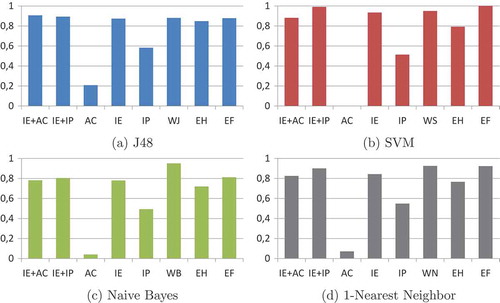
The results suggest a relative equilibrium in the predictive results of the MOGA IE+AC and the wrappers. These FS algorithms were able to generate several models with good predictive performance, while also reducing considerably the number of input features. Although Figure 7 suggests that IE+IP, IE and EF were also competitive, recall that EF used all features to learn from data and the remaining algorithms achieved low reducton in the number of features (Table 4).

Despite of the lower accuracies than those observed for the wrappers, the IE+AC algorithm has as benefits the independence of classifiers in the FS task. In addition, filter algorithms usually demand less running time than the wrapper approach (Liu and Motoda 2007), although we did not perform a running time analysis in this work.

One can find some possible relations between MOGA predictive results and data properties. For example, for three classification algorithms (J48, NB, and NN), IE+AC usually supports the building of better classifiers than the ones derived from IE+IP for datasets with less instances (n in Table 3). This finding suggests that IE+AC can deal better with scenarios with limited number of training instances. Another example suggests that, for three classification algorithms (SVM, NB and NN), wrapper FS is the best choice for FS when the number of instances per feature, i.e., is higher. As reduces, other algorithms highlight. This could suggest that the wrapper approach is not the best choice in harder scenarios, with less instances per feature (sparse datasets).

It is also useful to notice that, when AC is optimized in isolation, there are some severe reductions in the accuracy rates when compared to the use of all features. But, when combined to IE, which was conservative in feature reduction singly, the search was more controlled, able to reduce the number of features while still maintaining or in some cases improving the accuracy performances.

EH has also performed an effective combination of multiple ranking criteria for FS. Nonetheless, it does not have the support to automatically identify which number of features should be employed, as genetic algorithms solutions do. Another disadvantage is that EH is mainly designed for feature ranking algorithms, which in turn can rank redundant features similarly.

Trade-off PR vs accuracy

For better comparing the MOGA and SOGA filters, we investigate the trade-off graphs of Percentage of Reduction in the number of features vs the predictive performance achieved by the SVM classifier according to the comparison model described in Section 5.3. Results for the other classification models are summarized in Figure 8 and in the supplementary material available at https://db.tt/3iGgSTc5.

Figure 8. Total number of classifiers built using features selected by the MOGA and SOGA filters for each category related to the trade-off between percentage of reduction in the number of features and classification accuracy.

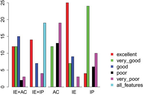
Table 7 organizes the FS algorithms for each dataset according to the five categories assigned by the model—excellent (▴▴▴), very good (▴), good (▴), poor (), and very poor (▾), as well as a category named all features (—), which labels those cases where no feature reduction was achieved. In addition, Figure 9 shows the correspondent plots. Note that the model for the dataset L can not be plotted because the error of the SVM classifier built without feature selection (EF) is higher than 0.5 (Table 5).

Table 7. Comparison of SVM models built after FS. This comparison involves categorizing the models into six categories regarding the compromise between dimensionality reduction and prediction performance: excellent (▴▴▴), very good (▴▴), good (▴), poor (), very poor (▾) and all features (—).

	A	C	D	G	▴▴▴	▴▴	▴		▾	—
IE+AC	▴▴▴	▴▴	▴	▾	1	1	1	0	1	0
IE+IP	—	▴	—	▴	0	0	2	0	0	2
IE	▴▴▴	▴▴	▴▴▴	▴▴	2	2	0	0	0	0
AC	▾	▾	▾	▾	0	0	0	0	4	0
IP	▾		▴▴	▾	0	1	0	1	2	0
	I	L	P	S	▴▴▴	▴	▴		▾	—
IE+AC	▴	▴▴▴	▴	▴▴	1	1	2	0	0	0
IE+IP	▴▴▴	▾	▴	▴▴▴	2	0	1	0	1	0
IE	▴▴▴	▾	▴▴	▴	1	1	1	0	1	0
AC	▾	▾	▴▴		0	1	0	1	2	0
IP	▴▴	▴▴▴	▴▴	▴▴	1	3	0	0	0	0
	Y	V	B	W	▴▴▴	▴▴	▴		▾	—
IE+AC	▴▴	▴	▴▴	▴	0	2	2	0	0	0
IE+IP	▴▴▴	—	—	—	1	0	0	0	0	3
IE	▴▴▴	▴▴▴	▴	▴▴▴	3	0	1	0	0	0
AC	▾	▾	▴▴	▾	0	1	0	0	3	0
IP	▴▴	▾	▴▴	▴▴	0	3	0	0	1	0

Figure 9. Graphic comparison of SVM models built after FS with statistical test results.

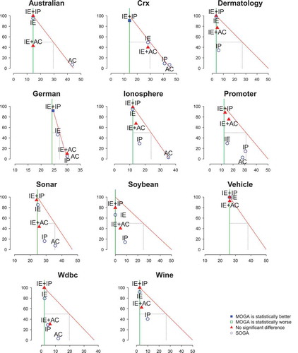
As illustrated in Figure 9 for SVM, no MOGA filter was significantly worse than its SOGA counterpart. Furthermore, the SVM classifiers correspondent to the MOGA were well categorized in most of the cases (Table 7), such that only one classifier was considered very poor (▾) for each filter. Nevertheless, as noted previously, IE+AC is better than IE+IP and reaches higher PR while maintaining a good accuracy performance.

SOGA IE also highlighted by supporting many classifiers with good trade-offs. However, as shown in Table 4, this filter often reaches smaller percentage of reduction in the number of features than IE+AC. This contributes to the obtainment of similar accuracy rates to those achieved by using all features.

While AC had several very poor results when optimized isolatedly, its combination with IE was very beneficial and improved the results achieved. This exemplifies the relevance of studying combinations of importance measures, even when one of the measures seems to be fruitless alone.

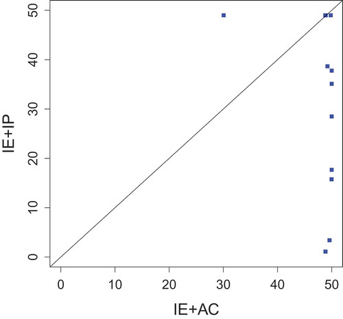
Non-dominated solutions

For comparing the multi-objective algorithms independently of the machine learning classification algorithms, we plotted graphs comparing the average number of non-dominated solutions obtained for each MOGA. The points in these graphs represent the 12 datasets studied, as exemplified in (Batista, Wang, and Keogh 2011) for another context. The coordinates of a point are the numbers of non-dominated solutions obtained by a given pair of MOGA. The MOGA with more non-dominated solutions can be considered the algorithm that addresses the most conflicting feature importance measures.

Figure 10 shows that IE+AC leads to more non-dominated solutions in the majority of the datasets, since the points are more concentrated toward its area (under the diagonal). Therefore, in addition to higher reductions in the number of features, IE+AC was also able to optimize more conflicting importance measures, an important characteristic concerning multi-objective optimization. This can also explain the good results obtained by this particular combination in FS.

Figure 10. Comparison between MOGA in terms of the number of non- dominated solutions.

Conclusion

This article presented a method for multi-objective optimization of multiple feature importance measures, by employing a multi-objective genetic algorithm grounded in the Pareto theory. Although the MOGA algorithm currently developed supports the optimization of six feature importance measures and their combinations, we performed in this article a deeper evaluation of two combinations of pairs of simple measures, highlighted as most promising in our previous work (Spolaôr, Lorena, and Lee 2011a, 2010b) and able to deal with both quantitative and qualitative features. In fact, the main differential of this work is a more complete description of the method and a uniform analysis of the most relevant experimental results, based on a wider range of datasets and importance measures than most of the 21 related papers found by a pioneer systematic review.

The experimental results show that some combinations of the measures in a filter feature selector can indeed capture some of the main patterns in a dataset, while reducing the number of features employed as input. As an appropriate trade-off between accuracy and reduction in the number of features is important for some classification applications, this can be considered a good result. In particular, the best combination was between a distance-based measure and a correlation-based measure. This behavior was verified for classification algorithms of different paradigms, which used the selected features as input to build predictive models. However, if the interest is to obtain the highest accuracy for a specific classification algorithm, the wrapper approach is more appropriate. Future work should include the comparison of some of the evaluated MOGA combinations with other meta-heuristics. Experimental evaluations with artificial and real datasets should also be performed. Finally, although a single solution from the Pareto front estimated by an MOGA is chosen in this work, a combination of the non-dominated solutions found could improve the results achieved.

Acknowledgments

We would also like to thank Aurora T. R. Pozo and Antonio R. S. Parmezan for their collaboration.

Additional information

Funding

The authors would like to thank the Brazilian National Council for Scientific and Technological Development (CNPq) (grants 482222/2013-1 and 308232/2011-9), the São Paulo Research Foundation (FAPESP) (grants 2012/22608-8 and 2009/12963-2), the Coordination for the Improvement of Higher Education Personnel (CAPES) and the Federal University of ABC for the financial support provided.

References

- Aha, D., and D. Kibler. 1991. Instance-based learning algorithms. Machine Learning 6:37–66. doi:10.1007/BF00153759.
- Arauzo-Azofra, A., J. M. Benitez, and J. L. Castro. 2008. Consistency measures for feature selection. Journal of Intelligent Information Systems 30 (3):273–92. doi:10.1007/s10844-007-0037-0.
- Asuncion, A., and D. J. Newman. 2007. UCI machine learning repository. University of California, Irvine, School of Information and Computer Sciences. Accessed June 1, 2010. http://www.ics.uci.edu/˜mlearn/MLRepository.html.
- Bache, K., and M. Lichman. 2013. UCI machine learning repository. University of California, Irvine, School of Information and Computer Sciences. Accessed June 1, 2014. http://archive.ics.uci.edu/ml.
- Batista, G. E. A. P. A., X. Wang, and E. J. Keogh. 2011. A complexity-invariant distance measure for time series. In SIAM International Conference on Data Mining, 699–710. Mesa, United States: SIAM.
- Bleuler, S., M. Laumanns, L. Thiele, and E. Zitzler. 2003. PISA — A platform and programming language independent interface for search algorithms. In Evolutionary multi-criterion optimization, ed C. M. Fonseca, P. J. Fleming, E. Zitzler, L. Thiele, and K. Deb, 494–508. Berlin: Springer Berlin Heidelberg.
- Deb, K., S. Agrawal, A. Pratap, and T. Meyarivan. 2000. A fast elitist nondominated sorting genetic algorithm for multi-objective optimization: NSGA-II. In Parallel problem solving from nature, ed M. Schoenauer, K. Deb, G. Rudolph, X. Yao, E. Lutton, J. Merelo, and H. Schwefel, 849–58. Berlin: Springer Berlin Heidelberg.
- Dwork, C., R. Kumar, M. Naor, and D. Sivakumar. 2001. Rank aggregation methods for the Web. In International Conference on World Wide Web, 613–22. Hong Kong, China: ACM.
- Freitas, A. A. 2004. A critical review of multi-objective optimization in data mining: A position paper. SIGKDD Explorations Newsletter 6 (2):77–86. doi:10.1145/1046456.1046467.
- Guyon, I., and A. Elisseeff. 2003. An introduction to variable and feature selection. Journal of Machine Learning Research 3:1157–82.
- Hall, M. A. 1999. Correlation-based Feature Selection for Machine Learning. PhD Thesis, University of Waikato - New Zealand.
- Hall, M. A.–. 2000. Correlation-based feature selection for discrete and numeric class machine learning. In International Conference on Machine Learning, 359–66. Stanford: Morgan Kaufmann.
- Han, J., and M. Kamber. 2011. Data mining: Concepts and techniques, 3rd ed. San Francisco: Morgan Kaufmann.
- He, X., D. Cai, and P. Niyogi. 2005. Laplacian score for feature selection. In Advances in Neural Information Processing Systems, 507–14. Cambridge, United States: MIT Press.
- Kitchenham, B. A., and S. Charters. 2007. Guidelines for performing systematic literature reviews in software engineering. Technical report. Evidencebased Software Engineering - United Kingdom.
- Kohavi, R., and G. H. John. 1997. Wrappers for feature subset selection. Artificial Intelligence 97 (1–2):273–324. doi:10.1016/S0004-3702(97)00043-X.
- Lee, H. D., M. C. Monard, and F. C. Wu. 2006. A simple evaluation model for feature subset selection algorithms. Inteligência Artificial 10 (32):9–17.
- Liu, C., and H. Shum. 2003. Kullback-Leibler boosting. In Computer Vision and Pattern Recognition, 587–94. Madison, United States: IEEE.
- Liu, H., and H. Motoda. 1998. Feature selection for knowledge discovery and data mining. Norwell: Kluwer Academic Publishers.
- Liu, H., and H. Motoda. 2007. Computational methods of feature selection. Boca Raton: Chapman & Hall/CRC.
- Liu, H., and R. Setiono. 1996. A probabilistic approach to feature selection - a filter solution. In International Conference on Machine Learning, 319–27. Bari, Italy: Morgan Kaufmann.
- Liu, H., and L. Yu. 2002. Feature selection for data mining. Arizona State University, Ira A. Fulton Schools of Engineering. Accessed June 1, 2010. http://www.public.asu.edu/˜huanliu/sur-fs02.ps.
- Mccallum, A., and K. Nigam. 1998. A comparison of event models for naïve bayes text classification. In Workshop on Learning for Text Categorization, 41–48. Madison, United States: AAAI Press.
- Mitra, P., C. A. Murthy, and S. K. Pal. 2002. Unsupervised feature selection using feature similarity. IEEE Transactions on Pattern Analysis and Machine Intelligence 24 (3):301–12. doi:10.1109/34.990133.
- Nahook, H. N., and M. Eftekhari. 2013. A feature selection method based on ∩ - fuzzy similarity measures using multi objective genetic algorithm. International Journal of Soft Computing and Engineering 3 (2):37–41.
- Prati, R. C. 2012. Combining feature ranking algorithms through rank aggregation. In International Joint Conference on Neural Networks, 1–8. Brisbane, Australia: IEEE.
- Press, W. H., S. A. Teukolsky, W. T. Vetterling, and B. P. Flannery. 1992. Numerical recipes in C: The art of scientific computing. Cambridge: Cambridge University Press.
- Robnik-Sikonja, M., and I. Kononenko. 2003. Theoretical and empirical analysis of ReliefF and RReliefF. Machine Learning 53 (1–2):23–69. doi:10.1023/A:1025667309714.
- Santana, L. E. A., L. Silva, and A. M. P. Canuto. 2009. Feature selection in heterogeneous structure of ensembles: A genetic algorithm approach. In International Joint Conference on Neural Networks, 1491–98. Atlanta, United States: IEEE.
- Saroj, J. 2014. Multi-objective genetic algorithm approach to feature subset optimization. In IEEE International Advance Computing Conference, 544–48. Gurgaon, India: IEEE.
- Scholkopf, B., and A. J. Smola. 2001. Learning with Kernels: Support vector machines, regularization, optimization, and beyond. Cambridge, United States: MIT Press.
- Spolaôr, N., A. C. Lorena, and H. D. Lee. 2010a. A systematic review of applications of multiobjective metaheuristics in feature selection (in Portuguese). Technical report. NOTE: An English version of the technical report can be requested to the authors. Federal University of ABC - Brazil.
- Spolaôr, N., A. C. Lorena, and H. D. Lee. 2010b. Use of multiobjective genetic algorithms in feature selection. In IEEE Brazilian Symposium on Artificial Neural Network, 146–51. São Bernardo do Campo, Brazil: IEEE.
- Spolaôr, N., A. C. Lorena, and H. D. Lee. 2011a. Multi-objective genetic algorithm evaluation in feature selection. In Evolutionary multi-criterion optimization, ed R. Takahashi, K. Deb, E. Wanner, and S. Greco, 462–76. Berlin: Springer Berlin Heidelberg.
- Spolaôr, N., A. C. Lorena, and H. D. Lee. 2011b. Multiobjective genetic algorithms for feature selection (in Portuguese). In Encontro Nacional de Inteligência Artificial, 938–49. Natal, Brazil: Brazilian Computer Society.
- Wang, C., and Y. Huang. 2009. Evolutionary-based feature selection approaches with new criteria for data mining: A case study of credit approval data. Expert Systems with Applications 36 (3):5900–08. doi:10.1016/j.eswa.2008.07.026.
- Wilson, D. R., and T. R. Martinez. 1997. Improved heterogeneous distance functions. Journal of Artificial Intelligence Research 6:1–34.
- Witten, I. H., and E. Frank. 2011. Data mining: Practical machine learning tools and techniques, 3rd ed. San Francisco: Morgan Kaufmann.
- Xue, B., L. Cervante, L. Shang, W. N. Browne, and M. Zhang. 2013. Multi objective evolutionary algorithms for filter based feature selection in classification. International Journal on Artificial Intelligence Tools 22 (4):1350024–1–1350024–31. doi:10.1142/S0218213013500243.
- Yang, J., and V. Honavar. 1998. Feature subset selection using a genetic algorithm. IEEE Intelligent Systems and Their Applications 13 (2):44–49. doi:10.1109/5254.671091.
- Zaharie, D., S. Holban, D. Lungeanu, and D. Navolan. 2007. A computational intelligence approach for ranking risk factors in preterm birth. In International Symposium on Applied Computational Intelligence and Informatics, 135–40. Timisoara, Romania: IEEE.
- Zeleny, M. 1973. An introduction to multiobjetive optimization. In Multiple criteria decision making, ed. J. L. Cochrane, and M. Zeleny, 262–301. Columbia, United States: University of South Carolina Press.