Very Fast C4.5 Decision Tree Algorithm

ABSTRACT

This paper presents a novel algorithm so-called VFC4.5 for building decision trees. It proposes an adaptation of the way C4.5 finds the threshold of a continuous attribute. Instead of finding the threshold that maximizes gain ratio, the paper proposes to simply reduce the number of candidate cut points by using arithmetic mean and median to improve a reported weakness of the C4.5 algorithm when it deals with continuous attributes. This paper will focus primarily on the theoretical aspects of the VFC4.5 algorithm. An empirical trials, using 49 datasets, show that, in most times, the VFC4.5 algorithm leads to smaller decision trees with better accuracy compared to the C4.5 algorithm. VFC4.5 gives excellent accuracy results as C4.5 and it is much faster than the VFDT algorithm.

Introduction

Decision trees are one of the most widely used classification techniques. Many variations of the decision tree algorithm were proposed in the literature (Saqib et al. 2015). They include Classification And Regression Tree (CART) (Breiman et al. 1984), Iterative Dichotomizer 3 (ID3) (Quinlan 1986), CHi-squared Automatic Interaction Detector (CHAID) (Kass 1980), and Conditional Inference Trees (Hothorn, Hornik, and Zeileis 2006). A decision tree is a classifier expressed as a recursive partition of the training instances. It is constructed in a top-down manner, in each iteration, the instance space is partitioned by choosing the best attribute to split them (Agrawal and Gupta, 2013; Patel and Singh 2015).

An attribute in a learning problem may be nominal (categorical), or it may be continuous (numerical). Numerical attributes with a very large, even infinite domain, become an important challenge in areas of pattern recognition, machine learning, and data mining. Mining data with numerical attributes require discretization before or throughout the process of model building (Garcia et al. 2013). A special kind of discretization is performed through the decision tree construction process. The decision tree algorithm uses binarization which splits the numerical values into two intervals (Yang and Chen 2016).

C4.5 is one of the best known and most widely used decision tree algorithms (Lu, Wu, and Bongard 2015). Its accuracy level is high enough, independently of the data volume to be processed. One of the latest studies that compares decision trees and other learning algorithms shows that C4.5 has a very good combination of error rate and speed (Hssina et al. 2014; Lim, Loh, and Shih 2000). Various studies identify the C4.5 algorithm as one of the top classifiers in data mining (Wu et al. 2008). The algorithm has the ability to handle an incomplete training dataset (Garca Laencina et al. 2015), and to prune the resulting decision tree in order to reduce its size and optimize the decision path. C4.5 also has the ability to deal with continuous attributes. It handles continuous attributes using the binarization process. Those attributes are replaced by the discrete ones using threshold values which separate data into two intervals (Behera and Mohapatra 2015; Kotsiantis 2013; Perner 2015).

Even for C4.5 and other algorithms that can directly deal with quantitative data, learning is often less efficient and less effective. Several researchers reported that the C4.5 algorithm contains some weakness in domains with continuous attributes. They offer evidence that it can be more benefited from continuous attributes by using a new discretization method, or by developing some process in the C4.5 binarization method (Chong et al. 2014; Quinlan 1996; Sumam, Sudheep, and Joseph 2013). In 2013, Sudheep, Sumam, and Joseph reported that the binarization process in C4.5 is computationally intensive (Sumam, Sudheep, and Joseph 2013). To perform binarization, the continuous attribute values are first sorted. This process is time consuming and it is not practical for large datasets. To sort the attribute values, the C4.5 algorithm uses the Quick Sort method with complexity . Despite this, several authors showed that the learning process may be dominated by sorting of continuous attribute values.

The generalization limit in domains with continuous attributes is the most important problem in the C4.5 algorithm. The selected threshold value can not reflect and judge the generalization capability of the continuous attribute. So, the C4.5 algorithm may use continuous attributes with a low generalization performance to split data. Deciding based on those attributes will increase the tree size and decrease the model accuracy. Liu and Setiono (Liu and Setiono 1995) reviewed and compared C4.5’s performance with Chi2 global discretization and concluded that Chi2 discretization is effective in improving performance. These authors found that Chi2 global discretization performed as well as C4.5 local discretization, and occasionally improved its accuracy (Liu and Setiono 1995). A recent research compares Multiple Scanning, and C4.5 discretization shows that using a cut point that reflects the data distribution can improve the decision tree performance. The authors proved that using Multiple Scanning discretized data yields more accurate and less complex decision trees in many cases (Grzymala- Busse and Mroczek, 2015). But, discretization as a preprocessing task neglects the correlation between the conditional attributes and the class attribute (Wang et al. 2015). Thus, the problem of dealing with continuous attributes could be addressed by choosing an appropriate threshold value that defines perfectly the interval borders. In this setting, we prose statistical mean and median as an alternative to threshold searching process in the C4.5 algorithm. In this paper, a new algorithm called Very Fast C4.5 (VFC4.5) is proposed.

The rest of the present paper is organized as follows: section 2 describes in details the C4.5 Binarization process. The new algorithm is denoted in section 3 with a mathematical formulation. Experimental investigations are drawn in section 5 and 6, where a set of tests are carried out to measure the efficiency of the VFC4.5 applied on different databases in comparison with the initial C4.5 algorithm, VFDT, and CART algorithms.

C4.5 algorithm

There have been many variations for decision tree algorithms. C4.5 is one of the well-known decision tree induction algorithms (Quinlan 2014). In 1993, Ross Quinlin proposed the C4.5 algorithm which extents the ID3 algorithm (Quinlan 1986). Using information gain ratio to select the best attribute, C4.5 avoids ID3’s bias toward features with many values that occurs (Ooi, Tan, and Cheah 2016; Zhu et al. 2014). C4.5 has the ability to handle continuous attributes by proposing two different tests in function of each attribute values type.

At the training stage, the C4.5 uses the top down strategy based on the divide and conquer approach to construct the decision tree (Liu and Gegov 2016). It maps the training set and uses the information gain ratio as a measurement to select splitting attributes and generates nodes from the root to the leaves. Every illustrating path from the root node to the leaf node forms a decision rule to determine which the class of a new instance is (Dai and Ji 2014). The root node contains the whole training set, with all training case weights equal to 1.0, to take into account unknown attribute values (Quinlan 2014). If all training cases of the current node belong to one single class, the algorithm terminates. Otherwise, if all training cases belong to more than one class, the algorithm calculates the information gain ratio for each attribute . The attribute with the highest information gain ratio is selected to split information at the node (Mu et al. 2017). For a discrete attribute , the information gain ratio is computed by splitting training cases of the current node in function of each value of (Ibarguren, Prez, and Muguerza 2015). If is a continuous attribute, a threshold value must to be found for the splitting (Pandya and Pandya 2015).

Given a node with instances, described by a matrix of continuous attributes where each row is an horizontal vector of attribute values pre-classified by a class which is an element of the vertical class vector . Consider a continuous attribute , the C4.5 algorithm selects the optimal cut point that maximizes information gain to divide samples in into two subsets: and . As can be seen from algorithm 1, attribute values should be sorted with ascending order first, only distinct values are retained to select the candidate cut points. Then, the algorithm identifies the candidate cut points Eq. (1):

(1)

For each CCP, samples in are split into two intervals and to compute the information gain Eq. (2) for all condidate cut points:

(2)

where the information entropy measures the class impurity and the amount of information, and symbol is the size of . Then, the optimal cut point Eq. (3) is selected as a threshold value for attribute :

(3)

Once threshold value is selected, the algorithm calculates the gain ratio to compare the discriminative ability of the candidate attributes and select the optimal one in order to split the current node Eq. (4).

(4)

where the split information is calculated as in Eq. (5)

(5)

The attribute that maximizes information gain ratio is selected as the best splitting feature, and the algorithm split the current node in function of the selected attribute. [!h]

Table

Algorithm 1 C4.5 Find threshold algorithm
1: Inputs: : matrix of continuous attributes;
2: Outputs:
: the optimal attribute;
: the optimal cut point;
3: For each attribute , do
4:  Sort attribute values
5:  Find all potential cut points
6:  For each cut point , do
7:   Calculate information gain
8:  end
9:  Select the optimal cut point
10:   Calculate splitting performance
11:   Calculate gain ratio
12: end
13: Select the optimal attribute and its cut point

Very fast C4.5 algorithm

When analyzing real valued data and estimating subsets in data distribution, measures of central tendency can be used to identify and separate populations with different characteristics. The mean and median have been utilized as a binary cut-off to estimate threshold values and then to identify data outliers in geochemical data (Reimann, Filzmoser, and Garrett 2005). Also, median-based binarization is recently used to perform feature selection (Sugiyama and Borgwardt 2017). Combined with variance, mean is used as a threshold value in decision tree induction (Sumam, Sudheep, and Joseph 2013). Thus, measures of central tendency have been presented in several research studies to deal with real valued data. However, several practical questions arise when dealing with arithmetic mean and median as a threshold value. It is important to identify cases where such a simple measures can separate data into two pure subsets and cases where it might fail. Also, it is crucial to measure the efficiency of mean and median-split based on different data distributions to investigate their sensitivity and stability. To answer all these questions, we start by discussing theoretical characteristics of both the mean and median.

Mean or average is the representative value of the whole group of data. The arithmetic can take any value not observed in the original set of data, which can improve the generalization ability of a cut point (Lewis 2012). In this setting, using the mean as a threshold value will improve the classification of unseen cases. The median is also widely used as a measure of central tendency, and it is the central value in the set of data. It divides the data into two equal halves. This measure is affected by the number of values observed in the distribution (Rubin 2012). As shown in Eq. (6), the arithmetic mean involves both distribution values () and number of observations (). That is why the mean is sensitive to the outlier values in a dataset, in such a case, the mean cannot deliver a relevant cut point. Whereas, as can be seen from Eq. (7), the median value is affected only by the number of observations (), it is not sensitive to outlier values. The presence of outlier data values or the shape of frequency distribution has a dramatic impact on mean value (Sharma 2012), that is why, in such cases arithmetic mean could be replaced by the median (Reimann, Filzmoser, and Garrett 2005).

(6)

(7)

In order to answer the research questions related to the performances of mean and median as a splitting criterion, and which of those techniques yields most precise cut points, we simulate seven different continuous distributions:

1. Scenario 1: The Cauchy distribution with the location value and the scale value .

2. Scenario 2: The exponential distribution with the rate value .

3. Scenario 3: The gamma distribution with the shape parameter and the scale rate .

4. Scenario 4: The log-normal distribution with the mean value and the standard deviation .

5. Scenario 5: The logistic distribution with the location value and the scale value .

6. Scenario 6: The normal distribution with the mean value and the standard deviation .

7. Scenario 7: The Weibull distribution with the shape value and the scale value .

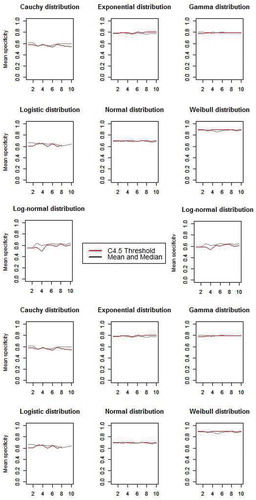
For each scenario 200 instances are simulated for two classes. Thus, for each scenario, according to the mean, median, and C4.5 threshold, three cut points are selected as can be seen from Figure 1. The previous simulations are repeated 10 times in order to compute sensitivities and specificities.

Figure 1. Seven different distributional scenarios.

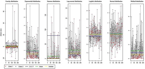
As can be seen from Figure 1, the three measures are strongly dependent to the data distribution except when the examples are normal distributed. As shown in scenario 6 (Normal distribution), mean, median, and C4.5 threshold provide the same cut points. Consider Table 2 which summarizes the accuracy rate for the three measures against the different scenarios, we can assume that in most cases C4.5 threshold results in better accuracies.

Table 1. Summary description of classification Datasets.

#	Dataset	Ex.	Atts.	Num.	Nom.	Cl.
1	Airlines	539383	8	3	5	2
2	Amazon commerce reviews	1500	10001	10000	1	50
3	Anneal	898	39	6	33	5
4	Appendicits	106	8	7	1	2
5	Audiology	226	70	0	70	24
6	Australian	690	15	8	7	2
7	Balance scale	625	5	4	1	3
8	Banana	5300	3	2	1	2
9	Bands	365	20	19	1	2
10	Bank marketing	4521	17	7	10	2
11	Bank marketing full	45211	17	7	10	2
12	Banknote authentication	1372	5	4	1	2
13	Blood transfusion service	748	5	4	1	2
14	Breast tissue	106	10	9	1	6
15	Clevheart disease	303	14	6	8	2
16	Contraceptive method choice	1473	10	2	8	3
17	Cnae 9	1080	857	856	1	9
18	Coil2000	9822	86	2	84	2
19	Cylinder bands	540	40	18	22	2
20	Flags	194	30	2	28	8
21	German credit	1000	21	8	13	2
22	Glass	214	10	9	1	6
23	Glioma16	50	17	16	1	2
24	Haberman	306	4	3	1	2
25	Heart disease hungarian	294	14	13	1	2
26	Heart disease processed	200	14	13	1	5
27	Hill valley with noise	1212	101	100	1	2
28	Hill valley without noise	1212	101	100	1	2
29	Leukemia haslinger	100	51	50	1	2
30	Lsvt voice rehabilitation	126	311	310	1	2
31	Lung cancer	32	57	56	1	3
32	Lymphography	148	19	3	16	4
33	Madelon	2600	501	500	1	2
34	Mammographic mass	961	6	5	1	2
35	Marketing	6876	14	13	1	9
36	Newthyroid	215	6	5	1	3
37	Ozone	2536	73	72	1	2
38	Page blocks	5473	11	10	1	5
39	Parkinsons	195	23	22	1	2
40	Pasture	36	23	22	1	3
41	Satimage	6435	37	36	1	6
42	Shuttle	57999	10	9	1	7
43	Spambase	4597	58	57	1	2
44	Spectheart	267	45	44	1	2
45	Squash stored	52	25	24	1	3
46	Tae	151	6	4	2	3
47	Thyroid allbp	2800	27	26	1	5
48	Unbalanced	856	33	32	1	2
49	Wholesale region	440	8	7	1	3

Table 2. Summary description of classification accuracy.

Distribution	Mean	Median	C4.5
Cauchy	75	77	78
Exponential	41	57	40
Gamma	42	80	40
Log-normal	90	68	66
Logistic	70	69	66
Normal	59	60	59
Weibull	30	18	20

In accordance with Table 2 and Figure 1, the cut points provided by the mean is slightly higher than the median cut point which is explained by the presence of extreme values in both scenario 4 and 7. Thus, in those cases, median cut points are more accurate than the mean ones. On the other hand, the mean cut point shows a smallest increase in error rate when instances are strongly fluctuated (i.e., scenario 5). Otherwise, a closer inspection of the results in Table 2 shows that in all scenarios there is at least one of the two cut points generated by mean and median that is slightly better or close to the C4.5 threshold cut point results. Thus, it is necessary to adopt both of mean and median as a candidate cut points and then to select the one that maximizes information gain. As shown in Figure 2, the associated sensitivities and specificities found by mean and median method are usually slightly higher than those detected with the C4.5 threshold technique. As already shown in Table 2 for the mean and median cut points, also for sensitivities and specificities from Figure 2, using both the mean and median as cut points can yield to slightly higher or the same results as obtained using the C4.5 threshold technique.

Figure 2. Specificity and sensitivity results.

The mean and median can communicate important information about data distribution. To cope with extreme values, we propose the use of mean and median as candidate cut points. In fact, in a class imbalanced dataset, extreme values may represent a minor class (Figure 1 (gamma distribution)). In this case, we suggest the mean as a threshold value. In other cases, median as it is not affected by extreme values can provide a more suitable threshold value (Figure 1 (Weibull distribution)). In this case, we provide two potential cut points, and then we compute information gain for both of them. It is important to look the dispersion of a dataset when interpreting the measures of central tendency, which is why we will use the cut point that maximizes information gain as a threshold value.

Algorithm description

The proposed VFC4.5 algorithm uses three processes that are responsible for achieving the tree construction: attribute selection, attribute binarization, and dataset splitting. The first and the last ones are the same as in the C4.5 algorithm. We introduce the use of mean and median as a candidate cut points in the attribute binarization process. Let be a matrix of continuous attributes, with instances and attributes. Algorithm 2 provides the optimal attribute and cut point to split the samples into two subsets. For each attribute, it calculates mean and median values. Once the splitting performances for both of mean and median is computed, the cut point that yields the highest value is set as a threshold value for the given attribute. Finally, algorithm 2 compares the splitting performances of all attributes and selects the optimal one.

Table

Algorithm 2 V FC4.5 Find threshold algorithm
1: Inputs: : matrix of continuous attributes;
2: Outputs:
: the optimal attribute;
: the optimal cut point;
3: For each attribute , do
4:  Calculate and ,
5:  Find all potential cut points
6:  For each cut point do
7:   Calculate information gain
8:  end
9:  Select the optimal cut point
10:   Calculate splitting performance
11:   Calculate gain ratio
12: end
13: Select the optimal attribute and its cut point

Analysis of time complexity

Suppose that there are cut points for each attribute . As described in algorithm 1, C4.5 starts with sorting the n examples for the m attributes which leads to a minimum complexity of . In steps 5, the algorithm selects cut points for each attribute , with a complexity of . Then in steps 6 to 9, it calculates the split information for each cut point which leads to a complexity of . Selecting the optimal cut point leads to a complexity of . Finally, the time complexity of algorithm 1 is .

The main advantage of the proposed algorithm is that it avoids the sorting process with complexity of , also for each attribute, there are only two cut points to evaluate. In algorithm 2, we start by computing mean and median for each attribute with a complexity of . In steps 6 to 9, the algorithm calculates the split information for each cut point which leads to a complexity of . Selecting the optimal cut point in algorithm 2 leads to a complexity of while there are only to cut points to evaluate. Thus, the time complexity of algorithm 2 is .

Experimental setup

In this section, experimental comparisons are conducted on 49 (UCI) machine learning datasets. In order to investigate the VFC4.5’s performance, the results are compared to those of C4.5, VFDT, and CART algorithms. This section specifies all the properties and issues related to datasets, validation procedure, and the parameters of used algorithms. We carried out experiments on 49 datasets taken from the UCI repository (UCI, 2015). Datasets with and without continuous attributes were used to train the VFC4.5 algorithm. Also, small and large datasets were used in order to investigate VFC4.5’s performance. Table 1 summarizes the main properties of the data. For each dataset, it includes the name, number of instances, number of numeric and nominal attributes, and number of classes. Ten-fold cross-validation was used to evaluate the performance of the algorithms. We used the J48 tree (the C4.5 decision tree implementation) of Weka software (Witten et al. 2016) to implement the new algorithm VFC4.5. Table 3 summarizes the parameters of the used classifiers.

Table 3. Parameters of algorithms.

Algorithm	Parameters
C4.5	Pruned tree: true, confidence factor: 0.25, examples per leaf: 2
	Reduced-error pruning: 3.
CART	Pruned tree: true, heuristic: true, examples per leaf: 2
	Reduced-error pruning: 5.
VFC4.5	Pruned tree: true, confidence factor: 0.25, examples per leaf: 2
	Reduced-error pruning: 3.
VFDT	Batch size:100, hoeffding Tie threshold: 0.05, leaf prediction
	Strategy: Naive Bayes adaptive, Decimal places: 2, Split criterion:
	Information gain split.

To demonstrate the usefulness and performance of our decision tree algorithm, we use accuracy, sensitivity and specificity as a performance measure to compare the generalization classification rate of VFC4.5 against C4.5, VFDT, and CART algorithms. Nevertheless, in decision tree, other measures are required to investigate the model complexity. We refer to the tree size, number of leaves, and time taken to build the model. Those performance measures will be adopted to measure the tree complexity. For all experiments, we have used the Wilcoxon test (Wilcoxon 1992) as a nonparametric statistical test. The Wilcoxon test is simple, safe, and robust test used for statistical comparisons of classifiers.

Analysis and empirical results

The collection of training sets, described previously, was applied to compare the performance of the algorithms. Table 4 presents the algorithms performance in term of correctly classified instances over the 49 datasets. Table 5 summarizes sensitivity and specificity. Similarly, Table 6 summarizes the results associated with tree size and number of leaves for each classifier considered. We use the test accuracies from Table 4 and run a Wilcoxon signed-rank test considering a level of significance equal to . Table 8 shows the Wilcoxon test results of all used measures. We carried out all possible comparisons using the performance measures in Table 4. Finally, Table 7 and Table 9 contain all detailed results for training time.

Table 4. Comparisons of testing accuracy results of different DT algorithms.

Dataset	C4.5	CART	VFC4.5	VFDT
1	66,287	—-	66,317	64,617
2	43,800	45,733	45,267	57,867
3	98,441	98,330	98,330	76,169
4	85,849	84,906	86,793	85,849
5	77,876	73,009	77,876	36,283
6	84,058	86,087	85,797	84,783
7	76,640	79,040	79,840	90,560
8	89,038	89,377	89,076	68,547
9	63,288	62,466	69,863	63,014
10	88,985	89,648	89,693	88,144
11	90,319	90,440	90,275	89,518
12	98,542	98,251	99,125	94,461
13	77,808	77,005	79,144	75,802
14	37,736	34,906	39,623	48,113
15	77,558	54,209	77,888	83,828
16	52,139	94,034	52,682	50,170
17	88,796	85,648	88,982	78,056
18	93,952	55,194	93,963	93,922
19	57,778	35,567	57,778	47,037
20	59,278	73,900	59,278	53,093
21	70,500	59,815	72,100	75,600
22	66,822	70,561	71,963	47,196
23	74,000	66,000	74,000	80,000
24	71,569	72,876	71,895	73,203
25	77,891	78,571	79,592	82,313
26	26,500	27,000	34,000	24,000
27	49,670	54,125	55,116	49,835
28	50,495	59,406	58,746	51,238
29	69,000	72,000	74,000	88,000
30	75,397	76,984	83,333	67,460
31	40,625	46,875	53,125	43,750
32	77,027	80,858	78,378	77,027
33	69,039	80,500	73,923	59,462
34	82,102	82,102	83,039	80,957
35	31,065	76,351	30,817	31,196
36	92,093	34,424	93,488	96,744
37	96,333	91,163	97,122	97,122
38	96,876	97,122	96,017	90,682
39	80,513	85,641	91,282	75,385
40	77,778	91,667	80,556	72,222
41	86,278	86,713	85,439	79,534
42	99,971	99,966	99,881	97,383
43	92,930	92,212	93,278	78,443
44	74,906	78,277	76,405	79,401
45	65,385	67,308	69,231	61,539
46	59,603	54,967	56,954	47,682
47	66,571	69,821	68,214	57,643
48	98,598	98,598	98,598	98,598
49	69,773	71,818	71,818	71,818
Mean	73,418	73,610	75,585	70,697

Table 5. Comparisons of sensitivity and specificity results of different DT algorithms.

#	C4.5		CART		VFC4.5		VFDT
	sens	spec	sens	Spec	sens	spec	sens	spec
1	0.662	0.663	0	0	0.661	0.633	0.645	0.646
2	0.442	0.438	0.494	0.457	0.437	0.453	0.615	0.579
3	0.984	0.984	0.982	0.983	0.983	0.983	0.58	0.762
4	0.849	0.858	0.84	0.849	0.859	0.868	0.861	0.858
5	0.736	0.779	0.677	0.73	0.736	0.779	0.567	0.363
6	0.841	0.841	0.862	0.861	0.858	0.858	0.85	0.848
7	0.732	0.766	0.742	0.79	0.724	0.798	0.835	0.906
8	0.892	0.89	0.894	0.894	0.891	0.891	0.691	0.685
9	0.631	0.633	0.612	0.625	0.693	0.699	0.397	0.63
10	0.875	0.89	0.881	0.896	0.871	0.897	0.859	0.881
11	0.895	0.903	0.895	0.904	0.894	0.903	0.878	0.895
12	0.985	0.985	0.983	0.983	0.991	0.991	0.945	0.945
13	0.764	0.778	0.742	0.77	0.762	0.791	0.661	0.758
14	0.382	0.377	0.381	0.349	0.381	0.396	0.447	0.481
15	0.776	0.776	0.426	0.542	0.773	0.779	0.838	0.838
16	0.521	0.521	0.884	0.94	0.521	0.527	0.521	0.502
17	0.904	0.888	0.863	0.856	0.903	0.89	0.86	0.781
18	0.897	0.94	0.556	0.552	0.902	0.94	0.899	0.939
19	0.334	0.578	0.127	0.356	0.334	0.578	0.52	0.47
20	0.57	0.593	0.725	0.739	0.57	0.593	0.561	0.531
21	0.687	0.705	0.592	0.598	0.708	0.721	0.746	0.756
22	0.67	0.668	0.693	0.706	0.712	0.72	0.509	0.472
23	0.742	0.74	0.667	0.66	0.742	0.74	0.823	0.8
24	0.687	0.716	0.674	0.729	0.679	0.719	0.68	0.732
25	0.777	0.779	0.782	0.786	0.783	0.796	0.826	0.823
26	0.275	0.265	0.308	0.27	0.333	0.34	0.148	0.24
27	0.497	0.497	0.541	0.541	0.551	0.551	0.498	0.498
28	0.255	0.505	0.594	0.594	0.588	0.587	0.521	0.512
29	0.691	0.69	0.722	0.72	0.74	0.74	0.88	0.88
30	0.748	0.754	0.763	0.77	0.831	0.833	0.64	0.675
31	0.406	0.406	0.511	0.469	0.511	0.531	0.449	0.438
32	0.776	0.77	0.809	0.809	0.76	0.784	0.798	0.77
33	0.69	0.69	0.805	0.805	0.709	0.739	0.595	0.595
34	0.822	0.821	0.821	0.821	0.821	0.83	0.81	0.81
35	0.29	0.311	0.749	0.764	0.287	0.308	0.269	0.312
36	0.921	0.921	0.299	0.344	0.925	0.935	0.967	0.967
37	0.957	0.963	0.911	0.912	0.943	0.971	0.943	0.971
38	0.967	0.969	0.943	0.971	0.957	0.96	0.923	0.907
39	0.802	0.805	0.856	0.856	0.911	0.913	0.697	0.754
40	0.772	0.778	0.933	0.917	0.806	0.806	0.724	0.722
41	0.861	0.863	0.862	0.867	0.851	0.854	0.819	0.795
42	1	1	1	1	0.999	0.999	0.983	0.974
43	0.929	0.929	0.922	0.922	0.926	0.933	0.799	0.784
44	0.751	0.749	0.691	0.783	0.75	0.764	0.63	0.794
45	0.66	0.654	0.718	0.673	0.72	0.692	0.63	0.615
46	0.595	0.596	0.548	0.55	0.571	0.57	0.485	0.477
47	0.66	0.666	0.696	0.698	0.66	0.682	0.559	0.576
48	0.972	0.986	0.972	0.986	0.972	0.986	0.972	0.986
49	0.529	0.698	0.516	0.718	0.516	0.718	0.516	0.718

Table 6. Comparisons of tree complexity results of different DT algorithms.

#	C4.5		CART		VFC4.5		VFDT
	#leaf	#size	#leaf	#size	#leaf	#size	#leaf	#size
1	147918	152908	0	0	111459	116168	3858	3967
2	312	623	134	267	317	633	1	1
3	35	47	10	19	52	69
4	3	5	2	3	4	7	0	0
5	32	54	22	43	32	54	2	2
6	31	58	6	11	18	32	2	2
7	52	103	13	25	73	145	1	1
8	46	91	39	77	124	247	5	7
9	34	67	9	17	52	103	1	1
10	104	146	10	19	134	198	5	7
11	1168	1716	43	22	816	1209	49	67
12	15	29	16	31	20	39	2	3
13	9	17	10	19	13	25	1	1
14	25	49	8	15	27	53	1	1
15	30	51	5	9	18	31	2	1
16	157	263	1	1	150	243	1	1
17	57	113	60	119	58	115	1	1
18	9	17	18	35	8	15	5	9
19	1	1	1	1	1	1	287	1
20	50	69	7	13	50	69	1	1
21	103	140	3	5	99	140	1	1
22	30	59	8	15	35	69	1	1
23	5	9	2	3	3	5	1	1
24	3	5	3	5	21	41	1	1
25	18	35	3	2	25	49	1	1
26	50	99	1	1	53	105	1	1
27	1	1	116	231	198	395	1	1
28	1	1	151	301	217	433	1	1
29	9	17	7	13	12	23	1	1
30	10	19	5	9	8	15	1	1
31	6	11	3	5	9	17	1	1
32	21	34	10	19	19	30	1	1
33	182	363	34	67	222	443	1	1
34	11	21	8	15	10	19	1	1
35	1180	2359	9	17	1133	2265	1	1
36	9	17	25	49	8	15	1	1
37	25	49	8	15	1	1	1	1
38	44	87	1	1	49	97	1	1
39	12	23	7	13	15	29	1	1
40	6	9	3	5	7	11	1	1
41	318	635	97	193	375	749	1	1
42	24	47	28	55	55	109	5	9
43	117	233	7	13	106	211	3	5
44	21	41	7	13	15	29	1	1
45	4	7	4	7	8	14	1	1
46	34	67	8	15	28	55	1	1
47	224	447	17	33	178	355	1	1
48	1	1	1	1	1	1	1	1
49	1	1	1	1	1	1	1	1

Table 7. Comparisons of training time results of different DT algorithms.

DataSet	C4.5	CART	VFC4.5	VFDT
1	660.28	—	357.79	3.86
2	187.35	617.78	110.03	363.35
3	0.16	0.65	0.14	0.06
4	0	0.02	0	0
5	0.01	0.03	0.01	0.05
6	0.01	0.05	0.05	0.02
7	0.01	0.06	0.05	0.01
8	0.05	0.42	0.02	0.04
9	0.01	0.04	0.02	0.01
10	0.35	3.83	0.4	0.2
11	2.98	61.99	1.19	0.61
12	0.01	0.07	0.02	0.01
13	0	0.04	0	0
14	0.02	0.02	0	0.01
15	0	0.06	0.03	0.03
16	0.02	0.1	0.07	0.01
17	2.17	12.55	1.52	4.84
18	3.7	65.02	2.23	0.72
19	0	0.02	0.01	0.02
20	0	0.01	0.01	0.01
21	0.02	0.06	0.06	0.01
22	0.01	0.02	0.01	0.01
23	0	0.01	0	0
24	0	0.01	0.01	0
25	0.02	0.02	0	0.01
26	0	0.03	0	0.01
27	0.05	4.32	0.16	0.1
28	0.05	3.82	0.12	0.08
29	0	0.04	0.02	0.01
30	0.06	0.23	0.02	0.05
31	0	0.01	0	0.01
32	0.01	0.02	0	0
33	4.01	14.02	0.62	1.15
34	0	0.07	0.01	0.01
35	0.57	6.21	0.48	0.31
36	0.01	0.01	0	0.01
37	0.24	3.02	0.27	0.17
38	0.19	2.16	0.26	0.17
39	0	0.03	0.02	0.01
40	0	0.01	0	0.01
41	0.69	13.02	0.47	1.15
42	1.93	103.14	1.17	2.97
43	0.89	14.31	0.83	0.29
44	0.02	0.03	0.02	0.01
45	0.01	0.13	0.01	0.03
46	0	0.02	0.01	0
47	0.23	3.13	0.2	0.14
48	0.04	0.16	0.08	0.02
49	0.02	0.05	0.01	0.01
Mean	17.677	19.393	9.764	7.767

Table 8. Wilcoxon’s signed rank tests of testing accuracies.

Method	C4.5	CART	VFC4.5	VFDT
C4.5	—-	0.3601	0.000003	0.08894
CART	—-	—-	0.01651	0.1637
VFC4.5	—-	—-	—-	0.001

Table 9. Comparisons of testing accuracy results on artificial data.

#	#instances	C4.5	CART	VFC4.5	VFDT
1	1000	0.01	0.01	0.01	0.01
2	10000	0.12	0.9	0.1	0.12
3	100000	0.52	2.6	0.31	0.11
4	1000000	0.97	5.01	0.69	5.07
5	5000000	21.73	—-	4.82	178.9

Once the accuracy results are presented in the mentioned tables, we can point out that the algorithms that achieve the highest accuracy on different datasets are quite different. For about half of the datasets, the decision trees created by the proposed algorithm overcome the solutions of all other algorithms. Generally, VFC4.5 outperforms the other algorithms, it increase the average accuracy level compared to C4.5, CART, and VFDT by, respectively, 2.09%, 1.93%, and 4.78%. Notably, as the VFC4.5 algorithm generally yields the highest accuracy, it also produces the highest values for specificities, therefore, the smallest values for sensitivities as mentioned in Table 5. Investigating the impact of the type of attributes, we observe that VFC4.5 has higher accuracy when the datasets contain only continuous attributes (line 9, 22, 26, 30, 31, and 39 from Table 3). In those cases, VFC4.5 outperforms all other algorithms. Besides, for mixed data, it is observed that VFC4.5 does not fail in all cases compared to C4.5, where results are quite similar. But clearly, CART has higher accuracy in those cases, independently of the number of classes (line 11, 16, 20, and 32 from Table 3). Also, it is observed that VFC4.5 can perform best on binary-class datasets. It yields higher accuracy on 26 datasets compared to C4.5 results, it only fails to improve the performance on dataset . However, this statement does not hold for datasets with limited sample size, where VFDT outperforms the results of all other algorithms (line 15, 23, 25, 29 and 44 from Table 3). in this setting, classes distribution has also an important impact on accuracy results. The proposed algorithm improves the C4.5 accuracy in class-imbalanced data with only few dominating classes (line 9, 22, 39 and 49 from Table 3). However, in cases where there are many dominating classes, the CART algorithm yields the highest accuracy. To investigate the difference between the algorithms and validate the previous results, we ran a Paired Wilcoxon’s signed rank test. The results are reported in Table 8. It can be seen that there are no significant differences between C4.5, CART, and VFDT algorithms. However, all of them are statistically different from the VFC4.5 algorithm. Furthermore, to attest the effectiveness of the VFC4.5 algorithm we make a second Wilcoxon signed rank test, which gives significance even at .

The VFC4.5 algorithm can also achieve reduction on the number of nodes, it outperforms the C4.5 results in 22 cases. In 20 datasets, the proposed algorithm improves both accuracy and tree size. But, the VFC4.5 creates more complex trees than CART and VFDT algorithms. This is explained by the higher accuracy achieved by the VFC4.5 algorithm.

Table 7 and Table 9 report the training time for real and artificial datasets. The results show that our algorithm performs faster than C4.5 in all cases. Compared to the VFDT results, the proposed algorithm fails to improve the training time in datasets with few examples. In contrast, for the datasets with high instances number (lines 4 and 5 from Table 9) and features (lines 2, 17, and 33 from Table 7), a significant time reduction has been achieved by using the VFC4.5 algorithm.

Conclusion

In this paper, we proposed a novel algorithm to speed up and improve the C4.5 algorithm performances. The results show that using mean and median as a threshold values can significantly speed up the process of binarization. But, also it improves the accuracy results. The results also show that for large number of training examples, VFC4.5 is faster than the VFDT algorithm and more accurate than C4.5. In contrast, experiments show that VFC4.5 fails in cases with few training examples and class imbalanced data with many dominating classes. For our future work, we plan to improve the VFC4.5 algorithm results on the two mentioned cases.

References

- Agrawal, G. L., and H. Gupta. 2013. Optimization of C4. 5 Decision Tree Algorithm for Data Mining Application. International Journal of Emerging Technology and Advanced Engineering 3 (3):341–45.
- Behera, H. S., and D. P. Mohapatra. Eds.., 2015. Computational Intelligence in Data Mining Volume 1: Proceedings of the International Conference on CIDM. 5-6 December 2015 Vol. 410. Springer.
- Breiman, L., J. Friedman, C. J. Stone, and R. A. Olshen. 1984. Classification and regression trees. CRC press.
- Chong, W. M., C. L. Goh, Y. T. Bau, and K. C. Lee. 2014. Advanced Applied Informatics (IIAIAAI), 2014 IIAI 3rd International Conference on, 930–35. IEEE.
- Dai, W., and W. Ji. 2014. A mapreduce implementation of C4. 5 Decision Tree Algorithm. International Journal of Database Theory and Application 7 (1):49–60.
- Garca Laencina, P. J., P. H. Abreu, M. H. Abreu, and N. Afonoso. 2015. Missing data imputation on the 5-year survival prediction of breast cancer patients with unknown discrete values. Computers in Biology and Medicine 59:125–33.
- Garcia, S., J. Luengo, J. A. Sez, V. Lopez, and F. Herrera. 2013. A survey of discretization techniques: Taxonomy and empirical analysis in supervised learning. IEEE Transactions on Knowledge and Data Engineering 25 (4):734–50.
- Grzymala-Busse, J. W., and T. Mroczek 2015. A comparison of two approaches to discretization: Multiple scanning and C4. 5. In International Conference on Pattern Recognition and Machine Intelligence (pp. 44–53). Springer International Publishing.
- Hothorn, T., K. Hornik, and A. Zeileis. 2006. Unbiased recursive partitioning: A conditional inference framework. Journal of Computational and Graphical Statistics 15 (3):651–74.
- Hssina, B., A. Merbouha, H. Ezzikouri, and M. Erritali. 2014. A comparative study of decision tree ID3 and C4. 5. International Journal of Advanced Computer Science and Applications 4 (2).
- Ibarguren, I., J. M. Prez, and J. Muguerza 2015. CTCHAID: Extending the Application of the Consolidation Methodology. In Portuguese Conference on Artificial Intelligence (pp. 572–77). Springer International Publishing.
- Kass, G. V. 1980. An exploratory technique for investigating large quantities of categorical data. In Applied statistics, 119–27.
- Kotsiantis, S. B. 2013. Decision trees: A recent overview. Artificial Intelligence Review 39 (4):261–83.
- Lewis, M. 2012. Applied statistics for economists. Routledge.
- Lim, T. S., W. Y. Loh, and Y. S. Shih. 2000. A comparison of prediction accuracy, complexity, and training time of thirty-three old and new classification algorithms. Machine Learning 40 (3):203–28.
- Liu, H., and A. Gegov. 2016. Induction of modular classification rules by information entropy based rule generation. In Innovative Issues in Intelligent Systems, 217–30. Springer International Publishing.
- Liu, H., and R. Setiono 1995. Chi2: Feature selection and discretization of numeric attributes. In Tools with artificial intelligence, proceedings., seventh international conference on (pp. 388–91). IEEE.
- Lu, Z., X. Wu, and J. C. Bongard. 2015. Active learning through adaptive heterogeneous ensembling. IEEE Transactions on Knowledge and Data Engineering 27 (2):368–81.
- Mu, Y., X. Liu, Z. Yang, and X. Liu. 2017. A parallel C4. 5 decision tree algorithm based on MapReduce. Concurrency and Computation. Practice and Experience 29:8.
- Ooi, S. Y., S. C. Tan, and W. P. Cheah. 2016. Temporal sampling forest: An ensemble temporal learner. In Soft Computing, 1–14.
- Pandya, R., and J. Pandya. 2015. C5.0 algorithm to improved decision tree with feature selection and reduced error pruning. International Journal of Computer Applications 117 (16).
- Patel, N., and D. Singh. 2015. An Algorithm to Construct Decision Tree for Machine Learning based on Similarity Factor. International Journal of Computer Applications 111:10.
- Perner, P. 2015. Decision tree induction methods and their application to big data. In Modeling and Processing for Next-Generation Big-Data Technologies (pp. 57–88). Springer International Publishing.
- Quinlan, J. R. 1986. Induction of decision trees. Machine Learning 1:81–106.
- Quinlan, J. R. 1996. Improved use of continuous attributes in C4. 5. Journal of Artificial Intelligence Research 4:77–90.
- Quinlan, J. R. 2014. C4. 5: Programs for machine learning. Elsevier.
- Reimann, C., P. Filzmoser, and R. G. Garrett. 2005. Background and threshold: Critical comparison of methods of determination. Science of the Total Environment 346 (1):1–16.
- Rubin, A. 2012. Statistics for evidence-based practice and evaluation. Cengage Learning.
- Saqib, F., A. Dutta, J. Plusquellic, P. Ortiz, and M. S. Pattichis. 2015. Pipelined decision tree classification accelerator implementation in FPGA (DT-CAIF). IEEE Transactions on Computers 64 (1):280–85.
- Sharma, J. K. 2012. Business statistics. Pearson Education India.
- Sugiyama, M., and K. M. Borgwardt. 2017. Significant Pattern Mining on Continuous Variables. arXiv preprint arXiv:1702.08694.
- Sumam, M. I., E. M. Sudheep, and A. Joseph. 2013. A Novel Decision Tree Algorithm for Numeric Datasets-C 4.5* Stat.
- UCI, UCI Machine Learning Repository, https://archive.ics.uci.edu/ml/datasets.html (2015).
- Wang, R., S. Kwong, X. Z. Wang, and Q. Jiang. 2015. Segment based decision tree induction with continuous valued attributes. IEEE Transactions on Cybernetics 45 (7):1262–75.
- Wilcoxon, F. 1992. Breakthroughs in Statistics. In Individual comparisons by ranking methods, 196–202. Springer New York.
- Witten, I. H., E. Frank, M. A. Hall, and C. J. Pal. 2016. Data Mining: Practical machine learning tools and techniques. Morgan Kaufmann.
- Wu, X., V. Kumar, J. R. Quinlan, J. Ghosh, Q. Yang, H. Motoda, … Z. H. Zhou. 2008. Top 10 algorithms in data mining. Knowledge and Information Systems 14 (1):1–37.
- Yang, Y., and W. Chen. 2016. Taiga: Performance optimization of the C4. 5 Decision Tree Construction Algorithm. Tsinghua Science and Technology 21 (4):415–25.
- Zhu, H., J. Zhai, S. Wang, and X. Wang. 2014. Monotonic decision tree for interval valued data. In International Conference on Machine Learning and Cybernetics, 231–40. Springer Berlin Heidelberg.