Determining the Natural Frequency of Cantilever Beams Using ANN and Heuristic Search

ABSTRACT

An artificial neural network (ANN) is used to model the frequency of the first mode, using the beam length, the moment of inertia, and the load applied on the beam as input parameters on a database of 100 samples. Three different heuristic optimization methods are used to train the ANN: genetic algorithm (GA), particle swarm optimization algorithm and imperialist competitive algorithm. The suitability of these algorithms in training ANN is determined based on accuracy and runtime performance. Results show that, in determining the natural frequency of cantilever beams, the ANN model trained using GA outperforms the other models in terms of accuracy.

Introduction

A lot of research has been conducted in determining the beam frequency and in floor vibration control (Hudson and Reynolds 2012; Morley and Murray 1993). Prediction of natural frequency is performed either by assuming the floor to act like a beam or a plate, and usually only the fundamental frequency is estimated, while the participating (or modal) mass estimation is based on a crude estimation of the mode shape (Middleton and Brownjohn 2010). Over the past few years, experimental and analytical methods have also been carried out to investigate the behavior of structural composite floors in terms of dynamic response, where modern computational tools have been implemented with the applications of finite element analysis (Behnia et al. 2013; Da Silva et al. 2003; Ellis 2001). Beavers (1998) used a finite element program to model single-bay joist-supported floors and to predict fundamental frequencies. Sladki (1999) used finite element modeling of steel composite floors to predict the fundamental frequency of vibration and the peak acceleration due to walking excitation. Alvis (2001) used finite element modeling of steel composite floors to predict peak accelerations due to sinusoidal loads.

As an alternative to conventional techniques, artificial neural networks (ANNs) have been applied in many different studies relating to vibrations of beam or floor systems and crack identifications since the natural frequency is frequently used as a parameter for detection of cracks in the structures. Using these techniques, the attention of researchers is to solve problems for which no analytic method is available, e.g., complicated nonlinear differential equations.

Multi-layer feed-forward ANNs trained using the back propagation (BP) algorithm have been used in several papers (Bağdatlı et al. 2009; Karlik et al. 1998; Özkaya and Pakdemirli 1999; Waszczyszyn and Ziemiański 2001). In Karlik et al. (1998), the nonlinear vibrations of an Euler-Bernoulli beam with a concentrated mass attached to it were investigated. Natural frequencies were calculated for different boundary conditions, mass ratios and mass locations as well as the corresponding nonlinear correction coefficients for the fundamental mode. The calculated natural frequencies and nonlinear corrections (by Newton–Raphson method) were used in training the ANN. For the case of clamped-clamped edge conditions of a beam-mass system, Özkaya and Pakdemirli (1999) calculated exact mode shapes and frequencies while the amplitude dependent nonlinear frequencies were found approximately using the method of multiple scales. The ANN model was obtained using exact natural frequency values and nonlinear correction coefficients. Waszczyszyn and Ziemiański (2001) applied ANN in analyzing the following problems: (1) bending analysis of elastoplastic beams, (2) elastoplastic plane stress problem, (3) estimation of fundamental vibration periods of real buildings, (4) detection of damage in a steel beam and (5) identification of loads applied to an elastoplastic beam. Bagdatli et al. (2009) investigated the nonlinear vibrations of stepped beams having different boundary conditions. The calculated natural frequencies and nonlinear corrections (by Newton–Raphson Method) were used for training the ANN model.

Similarly, neural network analysis and techniques were employed in Ghorban Pour and Ghassemieh (2009) to investigate the vertical vibration of the composite floor system subject to footstep loading, as well as in the work of Gerami, Sivandi Pour, and Dalvand (2012), where dynamic analysis and FEM were adopted to constitute the frequency equations of the fixed ends and cantilever steel beams.

To overcome limitations (e.g., being trapped in a local minimum) of the algorithms for training ANN (based on gradient-descent methods like back propagation (BP)), many researchers have employed heuristic optimization algorithms for ANN learning (Nikoo, Torabian Moghadam, and Sadowski 2015.). Examples of such heuristic algorithms used in ANN training include genetic algorithms (GA) (Hadzima-Nyarko et al. 2012; Liu et al. 2015), particle swarm optimization (PSO) (Dash 2015; Liao et al. 2015), artificial bee colony (ABC) (Kuru et al. 2016), imperialist competitive algorithm (ICA) (Chen, Chen, and Chang 2015; Sadowski and Nikoo 2014) or social-based algorithm (SBA) (Nikoo et al. 2016).

The use of heuristic optimization methods in the field of vibration of beam, either in solving optimization problems or in training ANNs can be found in Martell, Ebrahimpour, and Schoen (2005), Marinaki, Marinakis, and Stavroulakis (2010), and Kazemi et al. (2011).

In Martell, Ebrahimpour, and Schoen (2005), a novel experimental control approach was presented where a GA and a piezoelectric actuator were used to control the vibration of an aluminum cantilever beam. This set-up was based on a floor vibration problem, where the human perception of vibration dictates the sensitivities in the cost function of the GA. Marinaki, Marinakis, and Stavroulakis (2010) designed a vibration control mechanism for a beam with bonded piezoelectric sensors and actuator and applied three different variants of the PSO for the vibration control of the beam. Kazemi et al. (2011) used FEM for three natural frequencies of a cantilever beam for different locations and depths of cracks and then applied ANN, trained using PSO, in the process of crack identification of a cantilever beam.

The contributions of this paper are twofold: modeling the natural frequency of cantilever beams using an ANN model with three inputs (beam length, moment of inertia, and load applied on the beam) is investigated; and the suitability of three different heuristic optimization methods (GA, PSO and ICA) in training ANNs is analyzed in terms of accuracy and runtime performance.

The contributions of this paper are twofold: modeling the natural frequency of cantilever beams using an ANN model with three inputs (beam length, moment of inertia, and load applied on the beam) is investigated; and the suitability of three different heuristic optimization methods (GA, PSO and ICA) in training ANNs is analyzed in terms of accuracy and runtime performance.

The rest of this paper is organizes as follows. In section “Determination of beam frequency using dynamic analysis,” an overview of the dynamic analysis used to determine the natural frequency of beams is provided. Section “Soft computing methods implemented” provides a brief overview of the soft computing methods employed in this paper: ANN, GA, PSO and ICA. The experimental results and analysis are provided in section “Experimental analysis.” Finally, the paper is concluded with section “Conclusion.”

Determination of beam frequency using dynamic analysis

Vibration is more important than deflection control in designing buildings. The Design Guide method, which adopted the criterion given by Allen and Murray (1993), essentially requires two sets of calculations. Firstly, the frequencies of the beams, the girders, and then the entire bay need to be estimated. In general, it is assumed that the members are simply supported; however, cantilever sections are considered. Secondly, the peak acceleration due to walking is approximated by estimating the effective mass of the system and then calculating the peak acceleration due to a dynamic load of specific magnitude, oscillating at the lowest natural frequency of the system, applied at an anti-node of the system (Sladki 1999).

Given the importance of controlling vibration of floors, in developing the terms of steel building design codes such as AISC America Regulations (Murray, Allen, and Ungar 1997), Canada CSA Regulations (CSA-Standard 1999), Steel Building Design, and Construction Regulations of Iran, a simple equation to determine the frequency of the beam is introduced.

In calculating the natural frequency of steel built-in beams, assuming the beam is placed under variable transverse load to time and place, the response of displacement in the structure compared to vertical change of dimension on longitudinal axis of beam in page load is a function of these two dimensions where each variable is independent of the other variable (Przybylski 2009). To determine the natural frequency of in-built beams, the governing equation on the vibration of these beams with various conditions and properties using dynamic analysis must initially be obtained (Gerami, Sivandi Pour, and Dalvand 2012).

Equation (1) demonstrates the effects of axial force and total vibration equation (Housner 1975):

(1)

where EI is the flexural rigidity; v is the shear force; N is the axial force; p is the vertical load; m is the mass; x is the beam length and t the time.

Ignoring the effects of axial forces and assuming the moment of inertia of the beam to be constant, Equation (1) converts to Equation (2) (Housner 1975):

(2)

In order to solve Equation (2), in the case of free vibration, a constant mass and flexural rigidity in the beam is assumed, and using the separation of variables method for solving partial differential equations, the final equation will be written as Equation (3) (Housner 1975):

(3)

where is the function of beam length, and Y is a function of oscillator vibrations (Gerami, Sivandi Pour, and Dalvand 2012).

Beam or joist and girder panel mode natural frequencies can be estimated from the fundamental natural frequency equation of a uniformly loaded, simply-supported, beam (Murray, Allen, and Ungar 1997):

(4)

where:

f_n – fundamental natural frequency [Hz],

g – acceleration of gravity [9.86 m/s²],

E_s – modulus of elasticity of steel,

I_t – transformed moment of inertia; effective transformed moment of inertia, if shear deformations are included,

w – uniformly distributed weight per unit length (actual, not design, live and dead loads) supported by the member,

L – member span.

Equation (4) can be rewritten and AISC and CSA regulations, to determine the natural frequency of steel beams, have introduced Equation. 5 (CSA-Standard 1999; Murray, Allen, and Ungar 1997):

(5)

where Δ is midspan deflection of the member relative to its supports due to the weight supported.

Considering that the elasticity module of steel (E_s) in used profiles in the construction industry is a constant 2 × 10⁶ kg/cm², this value has been included in the β coefficient (Gerami, Sivandi Pour, and Dalvand 2012):

(6)

The tenth Issue of National Building Regulations of Iran and CSA-Standard have recommended the use of Equation (6) to calculate the frequency of simple beams (CSA-Standard 1999):

(7)

where I is the momentum inertia of the beam (cm⁴), P is the dead applied load in terms (kg/m),

L is the bay length (m), and f is the natural frequency of first mode (Hz) (CSA-Standard 1999).

Soft computing methods implemented

In situations where unknown functional relations need to be modeled or nonlinear regression needs to be performed, soft computing methods have shown to be advantageous over analytical methods. In this paper, ANN is used to model the unknown functional relationship between the frequency of the first mode, representing the dependent (output) parameter and the beam length, the moment of inertia, and the load applied on the beam as independent (input) parameters. A standard training algorithm of ANN is the BP algorithm, which is a deterministic optimization algorithm.

Optimization algorithms are basically iterative in nature and as such the quality of an optimization algorithm is determined by the quality of the result obtained in a finite amount of time. Deterministic algorithms are designed in such a way that the optimal solution is always found in a finite amount of time. Thus, deterministic algorithms can only be implemented in situations where the search space can efficiently be explored. Deterministic optimization algorithms also depend on the initial value(s) of the parameter(s) being optimized. In situations, where the search space cannot be efficiently explored, e.g., a high dimensional search space, implementing a deterministic algorithm might result in an exhaustive search, which would be unfeasible due to time constraint. In order to overcome this problem, heuristic optimization methods are often implemented. Heuristic optimization methods generally optimize a problem by iteratively trying to improve a candidate solution with respect to a given measure of quality. They make few or no assumptions about the problem being optimized and can search very large spaces of candidate solutions. However, probabilistic algorithms provide no guarantee of an optimal solution being found, only a good solution in a finite amount of time.

The BP algorithm is a gradient-based method, and as such determines the optimal weights of the ANN. However, this optimal solution depends on the initial values of the weights of the ANN, which are generated randomly. Thus, this optimal solution may represent a local optimum. In order to increase the chance of attaining the global optimal solution, or a solution close to the global optimum, heuristic optimization methods can be used especially in situations where a large number of parameters need to be optimized.

In this paper, four completely different heuristic optimization methods are compared and their suitability in ANN training is determined based on accuracy and runtime performance. All the four heuristic algorithms belong to the category of evolutionary algorithms (EA). They are all population based algorithms and as such, always work on a set of candidate solutions during each iteration of the algorithm. The number of candidate solutions, referred to herein as N is usually kept constant during the execution of the algorithm. The objective function, which is the mean squared error (MSE) between the ANN output and the actual output, will be referred to as the fitness function or the quality of the parameter vector.

A brief overview of the soft computing methods implemented in this paper is provided in the following subsections.

Artificial neural network (ANN)

Among the many ANN structures that have been studied, the most widely used network structure is the multilayer feed-forward network, which is the structure implemented in this paper. The basic structure of an ANN model is usually comprised of three distinctive layers, the input layer, where the data are introduced to the model, the hidden layer or layers, where data are processed, and the output layer, where the results of the ANN are produced (Figure 1). Each layer consists of nodes referred to as neurons. In a feed-forward neural network, information moves only in one direction, forward, from the input neurons, through the hidden nodes to the output neurons. Each neuron is connected to other neurons in the proceeding layer. Apart from the neurons in the input layer, which only receive and forward the input signals to the other neurons in the hidden layer, each neuron in the other layers consists of three main components; weights, bias, and an activation function, which can be continuous, linear or nonlinear. Standard activation functions include, nonlinear sigmoid functions (logsig, tansig) and linear functions (poslin, purelin).

Figure 1. The topology of a feed-forward ANN with three neurons in the input layer, five neurons in the first hidden layer, four neurons in the second hidden layer and one neuron in the output layer (3–5-4–1).

Once the architecture of a feed-forward neural network has been defined (number of layers, number of neurons in each layer, activation function for each layer), the weights and bias levels are the only free parameters that can be adjusted. Modifying these parameters changes the output values of the network. In order to model a given real function or process, the weights and bias levels are adjusted to obtain the desired network output within an error margin. This adjustment procedure is referred to as training. Different training algorithms are implemented depending on the type of neural network implemented. The best known ANN training algorithm is the BP algorithm. This training algorithm distributes the network error in order to arrive at a best fit or minimum error. Details regarding the different types of ANN structures as well as training algorithms can be found in Haykin (1999) and Bishop (2006).

Genetic algorithm (GA)

Concepts from biology, genetics and evolution are freely borrowed to describe GA. A candidate solution (which is often a parameter vector) is referred to as an individual, an element of the individual is referred to as a gene, the set of candidate solutions is referred to as a population and an iteration of the algorithm is referred to as a generation. During the execution of the algorithm, a candidate solution or parent is modified in a particular way to create a new candidate solution or child.

Using these terms, an overview of a basic evolutionary computation algorithm can be provided. The basic EA first constructs an initial population, then iterates through three procedures. It first assesses the quality or fitness of all the individuals in the population. Then, it uses this fitness information to reproduce a new population of children. Finally, it merges the parents and children in some fashion to form a new next-generation population, and the cycle continues. The stopping condition of the algorithm is often defined in a few ways such as: (1) limiting the execution time of the algorithm. This is normally done either by defining the maximum number of iteration (k_max), or by limiting the maximum number of fitness function evaluations (fit_EVAL); (2) the best fitness value (f_BEST) does not change appreciably over successive iterations; (3) or attaining a pre-specified objective function value. The best solution, corresponding to f_BEST, found by the EA is referred to herein as x_BEST.

One of the first EA is GA invented by (Holland 1992). The standard GA consists of three genetic operators: selection, crossover and mutation. During each generation, parents are selected using the selection operator. The selection operator selects individuals in such a way that individuals with better fitness values have a greater chance of being selected. Then new individuals, or children, are generated using the crossover and mutation operators. There are many variants of GA due to the different selection, crossover and mutation operators proposed, some of which can be found in Holland (1992), Goldberg (1989), Baker (1987) and Srinivas and Patnaik (1994). The GA analyzed in this paper is available in the Global Optimization Toolbox of Matlab R2010a. The selection function used in this paper is the stochastic universal sampling (SUS) method (Baker 1987). In the SUS method, parents are selected in a biased fitness-proportionate way such that fit individuals get picked at least once. The crossover operator used in this paper is the scattered or uniform crossover method. Assuming the parents and have been selected, a random binary vector or mask is generated. The children and are then formed by combining genes of both parents. This recombination is defined by Equations and :

(8)

(9)

The number of children to be formed by the crossover operator is provided by a user defined parameter P_crossover, which represents the fraction of the population involved in crossover operations. The crossover operator tends to improve the overall quality of the population since better individuals are involved. As a result, the population will eventually converge, often prematurely, to copies of the same individual. In order, to introduce new information, i.e., move to unexplored areas of the search space, the mutation operator is needed. The Uniform mutation operator is used in this paper. Uniform mutation is a two-step process. Assuming an individual has been selected for mutation, the algorithm selects a fraction of the vector elements for mutation. Each element has the same probability, R_mutation, of being selected. Then, the algorithm replaces each selected element by a random number selected uniformly from the domain of that element. In order to guarantee convergence of GA, an additional feature—elitism is used. Elitism ensures that at least one of the best individuals of the current generation is passed on to the next generation. This is often a user defined value, N_elite, and indicates the top N_elite individuals, ranked according to their fitness values, that are copied on to the next generation directly.

Particle swarm optimization (PSO)

PSO belongs to the set of swarm intelligence algorithms. Even though there are some similarities to EA, it is not modeled after evolution but after swarming and flocking behaviors in animals and birds. It was initially proposed by (Kennedy and Eberhart 1995). A lot of variations and modifications of the basic algorithm have been proposed ever since (Liang et al. 2006; Zambrano-Bigiarini, Clerc, and Rojas 2013). A candidate solution in PSO is referred to as a particle, while a set of candidate solutions is referred to as a swarm. A particle i is defined completely by three vectors: its position, x_i, its velocity, v_i, and its personal best position x_i,_Best. The particle moves through the search space defined by a few simple formulae. Its movement is determined by its own best known position, x_i,Best, as well as the best known position of the whole swarm, x_BEST. First, the velocity of the particle is updated using Equation :

(10)

then the position is updated using Equation :

(11)

where r₁ and r₂ are random numbers generated from U(0,1), c₀ is the inertia weight, and c₁ and c₂ are the cognitive and social acceleration weights, respectively. Modern versions of PSO such as the one analyzed in this paper do not use the global best solution, x_BEST, in Equation but rather the local best solution x_i,_LBest (Zambrano-Bigiarini, Clerc, and Rojas 2013; Clerc 2012). Hence, the velocity update equation is given by

(12)

The local best solution of a given individual is determined by the best-known position within that particle’s neighborhood. Different ways of defining the neighborhood of a particle can be found in Kennedy (1999), Kennedy, Eberhart, and Shi (2001), Kennedy and Mendes (2002) and Zambrano-Bigiarini, Clerc, and Rojas (2013). The analyzed PSO algorithm in this paper uses an adaptive random topology, where each particle randomly informs K particles and itself (the same particle may be chosen several times), with K usually set to 3. In this topology, the connections between particles randomly change when the global optimum shows no improvement (Zambrano-Bigiarini, Clerc, and Rojas 2013; Clerc 2012).

Imperialist competitive algorithm (ICA)

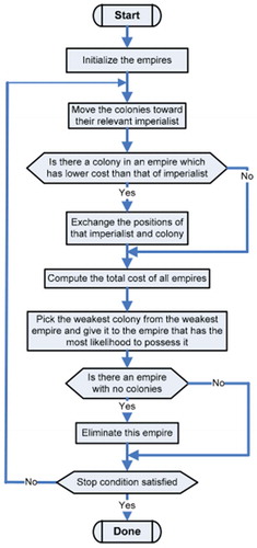
ICA represents a heuristic optimization method based on the mathematical modeling of socio-political development process (Sadowski and Nikoo 2014). Each possible solution is referred to as a country. The cost function of the optimization problem determines the power of each country. Depending on their power, some of the best initial countries are selected as imperialists. The remaining countries are referred to as colonies. Depending on their power, the imperialists attract the colonies to themselves and start forming empires. The total power of an empire depends on both its constituents (i.e., imperialist countries and their colonies) (Atashpaz-Gargari et al. 2009). Mathematically speaking, this dependence is modeled with the definition of imperial power as the total power of the imperialist country plus a percentage of the average power of the colonies. With the formation of the first empires, imperial competition starts between them, each colonial empire that does not succeed in this competition and increases its power (or at least prevents from reduction of its influence) will be removed from the colonial competition. The survival of an empire depends on its power to attract the colonies of the rival empires and bringing them under its control. As a result, during the imperial competition, the power of larger empires will increase and weaker empires will be eliminated. To increase power, empires will be forced to develop their colonies.

The three main operators of ICA are assimilation, revolution and competition. Assimilation causes the colonies of each empire to get closer to the imperialist state in the space of socio-political characteristics (optimization search space). Revolution, on the other hand, brings about sudden random changes in the position of some of the countries in the search space. During assimilation and revolution, the current imperialist state of the empire is replaced by a colony if the colony attains a better position than the imperialist. Due to competition, based on their power, all the empires have a chance to take control of one or more of the colonies of the weakest empire (Atashpaz-Gargari and Lucas 2007). The Imperialist Competitive Algorithm is shown in Figure 2.

Figure 2. Imperialist competitive algorithm flowchart (Atashpaz-Gargari and Lucas, 2007).

Experimental analysis

In this section, an overview of the data used as well as the results of the modeling procedures is provided. One hundred samples with different characteristics and frequencies are analyzed. The data used was generated by Gerami, Sivandi Pour, and Dalvand (2012). The beam length, the beam moment of inertia, the load applied to the beam as well as the frequency of the first mode in the cantilever beams represent the data used in modeling. The statistical properties of the data in are shown in Table 1.

Table 1. The characteristics of parameters used in first mode frequency of cantilever beams for different models (Gerami, Sivandi Pour, and Dalvand 2012).

Parameter name	Type of parameter	Unit	Maximum	Minimum	Standard deviation	Mean
Frequency of first mode	Output	Hz	399.34	17.7	69.9818	108.104
Load on the beam	Input	kg/m	3100	300	741.743	1424.6
Moment of inertia	Input	cm^4	256,887	246	79,109.1	55,699.1
Length of beam	Input	m	2	0.4	0.47411	1.087

For the ANN model to achieve better and more accurate results in the models, all the input and output parameters are normalized and scaled within the interval [−1, +1] (Ramezani, Nikoo, and Nikoo 2015).

The research process

As mentioned earlier, a feed-forward ANN is used in this research with the input parameters of network being the beam length, the beam’s moment of inertia and the load applied on the beam, while the frequency of the first mode in cantilever beams is regarded as the output. Of the 100 data models, 70% were used for training, and 30% of them were used to test the network. Determining the best ANN structure and number of neurons is a problem of its own (Bishop 2006) and is not the focus of this paper. If too small a network is chosen, the ANN is unable to model the functional relation between the input and the output, while too large a network results in the ANN over-fitting the data. After testing a few structure types, the ANN with an input layer of three neurons, two hidden layers each with five neurons and an output layer with one neuron (3–5-5–1) was deemed as suitable. tansig was used as the transfer function of all the neurons in the hidden layers while satlins was used as the transfer function of the output layer. Training such network structure implies optimizing the 56 neural network weights and biases in order to minimize the network output error.

In order to provide a fair comparison between the three heuristic methods (GA, PSO and ICA) used in training the ANN model, similar conditions needed to be provided: the same initial ANN networks were provided to each method and all three methods were limited to the same number of fitness function evaluations. Due to the nature of each algorithm, limiting the number of fitness evaluations was achieved simply by limiting the number of iterations for each algorithm. All the experiments were performed in MATLAB 2010a. The neural networks were generated using the Neural Network Toolbox in Matlab while GA was run using the Global Optimization Toolbox in Matlab as well. The code for PSO and ICA was downloaded from the internet.¹ The algorithm specific control parameters are provided in Table 2.

Table 2. Algorithm specific control parameter values used in the experiments.

Algorithm	Control parameters
GA	Nelite = 2; Pcrossover = 0.8; Rmutation = 0.01
PSO	;
ICA	Number of imperialists = 10% of the number of countries

The mean squared error (MSE), the coefficient of determination (R²) and the mean absolute error (MAE) are used as performance indicators of the trained models. These indicators are generated using the train data set and the test data set and compared with each other.

Since all the implemented optimization algorithms are population based, they require an initial set of possible solutions to be generated. It should be noted that for the 3–5-5–1 ANN model structure, a possible solution is represented by a real valued vector of 56 elements, each representing a particular weight or bias of the ANN model. Four experiments were performed in all. The experiments differed by the size of initial set of possible solutions generated (N_set = 20, 40, 100 and 400). For each fixed initial set, each optimization algorithm was implemented for 1000 iterations. Since these algorithms are probabilistic in nature, this procedure was repeated 10 times, i.e., 10 trial runs were performed. An overview of the experimental procedure is shown in Figure 3. The results obtained on the dataset used for training for the different initial set sizes and for all trial runs are presented in Table 3–6 and shown with the aid of box plots in Figure 4.

Table 3. Statistical data for all trial runs during ANN training (N_set = 20).

	MSE				MAE				R^2
	Min	Max	Mean	Median	Min	Max	Mean	Median	Min	Max	Mean	Median
GA	0.0303	0.0530	0.0415	0.0415	0.1146	0.1568	0.1405	0.1430	0.6637	0.8074	0.7363	0.7365
PSO	0.0264	0.0523	0.0394	0.0432	0.0889	0.1712	0.1296	0.1412	0.6679	0.8320	0.7500	0.7255
ICA	0.0375	0.0709	0.0526	0.0536	0.1414	0.2171	0.1704	0.1637	0.5502	0.7617	0.6657	0.6599

Table 4. Statistical data for all trial runs during ANN training (N_set = 40).

	MSE				MAE				R^2
	Min	Max	Mean	Median	Min	Max	Mean	Median	Min	Max	Mean	Median
GA	0.0219	0.0350	0.0296	0.0293	0.0884	0.1402	0.1114	0.1052	0.7776	0.8610	0.8116	0.8141
PSO	0.0298	0.0548	0.0460	0.0482	0.1115	0.1708	0.1491	0.1537	0.6523	0.8106	0.7076	0.6940
ICA	0.0274	0.0459	0.0381	0.0399	0.1216	0.1507	0.1339	0.1319	0.7084	0.8258	0.7581	0.7466

Table 5. Statistical data for all trial runs during ANN training (N_set = 100).

	MSE				MAE				R^2
	Min	Max	Mean	Median	Min	Max	Mean	Median	Min	Max	Mean	Median
GA	0.0254	0.0397	0.0290	0.0260	0.0938	0.1240	0.1024	0.0960	0.7476	0.8388	0.8156	0.8345
PSO	0.0430	0.0512	0.0473	0.0474	0.1436	0.1655	0.1533	0.1504	0.6749	0.7271	0.6999	0.6992
ICA	0.0275	0.0372	0.0317	0.0318	0.1052	0.1273	0.1178	0.1177	0.7634	0.8254	0.7985	0.7982

Table 6. Statistical data for all trial runs during ANN training (N_set = 400).

	MSE				MAE				R^2
	Min	Max	Mean	Median	Min	Max	Mean	Median	Min	Max	Mean	Median
GA	0.0154	0.0359	0.0262	0.0283	0.0830	0.1219	0.1037	0.1015	0.7716	0.9017	0.8331	0.8199
PSO	0.0455	0.0502	0.0472	0.0464	0.1391	0.1608	0.1516	0.1515	0.6812	0.7113	0.7005	0.7054
ICA	0.0232	0.0319	0.0271	0.0273	0.1046	0.1216	0.1132	0.1134	0.7971	0.8522	0.8278	0.8268

Figure 3. Overview of the experimental procedure used in comparing the three heuristic methods.

Figure 4. Box plot of the MSE values obtained for all trial runs during ANN training for (a) N_set = 20; (b) N_set = 40; (c) N_set = 100; (d) N_set = 400.

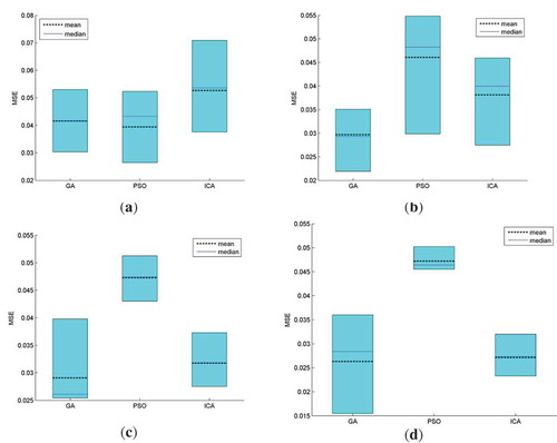
Looking at the results, it can be seen that for N_set = 20, the best model is obtained when training is performed using PSO, followed by GA and then ICA. However, for the other situations when N_set = 40, 100 and 400 the best model is obtained when training is performed using GA, followed by ICA and then PSO. Looking at Figure 4., it can be concluded that in general, increasing the initial set of possible solutions, N_set, the variance of the final MSE for all trial runs decreases when training is performed using PSO and ICA. The best model can generally be obtained by increasing the size of N_set. For each of the three training methods, the model obtained from the best trial run represents the best trained model. This model has the minimum MSE, minimum MAE and maximum R².

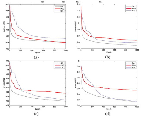
Figure 5 shows the MSE values for each iteration of the best trial run for each of the three training methods while Figure 6 shows the average MSE values for each iteration of all 10 trial runs for each of the three training methods. Analyzing Figures 5–6, it can be concluded that GA converges much faster than the other two methods and provides the best result for all iterations. PSO converges faster than ICA for the first 200 or so iterations after which better results are obtained using ICA.

Figure 5. MSE values for each iteration of the best trial run for each of the three training methods: (a) N_set = 20; (b) N_set = 40; (c) N_set = 100; (d) N_set = 400.

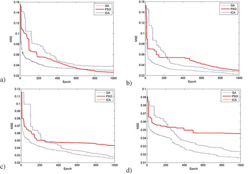
Figure 6. Average MSE values for each iteration of all 10 trial runs for each of the 3 training methods for (a) N_set = 20; (b) N_set = 40; (c) N_set = 100; (d) N_set = 400.

The mean training time per trial run is provided in Table 7. For N_set = 20, 40, and 100, the average training time per trial run (of 1000 iterations) per population size is approximately 37s, 27s and 22s for GA, PSO and ICA respectively. There is a slight increase, however, for N_set = 400 where the average training time per trial run per population size is approximately 47s, 36s and 28s for GA, PSO and ICA, respectively. It should be noted that these values should be taken with reserve since all simulations were performed in Matlab and is not in real time. They, however, give an indication of the complexity of the training method.

Table 7. Average training time per trial run.

Nset	Average training time (s)
	GA	PSO	ICA
20	747	545	442
40	1499	1093	891
100	3682	2731	2175
400	18,757	14,274	11,245

The quality of the best models obtained for each of the three training methods is determined by using the test data on these models. The results obtained on the test dataset are shown in Table 8.

Table 8. Performance of the best trained models on test data.

	Nset = 20			Nset = 40			Nset = 100			Nset = 400
	MSE	MAE	R^2	MSE	MAE	R^2	MSE	MAE	R^2	MSE	MAE	R^2
GA	0.0667	0.1771	0.7174	0.0597	0.1486	0.7469	0.0533	0.1439	0.7740	0.0747	0.1887	0.6833
PSO	0.0392	0.1127	0.8336	0.0438	0.1295	0.8142	0.0564	0.1627	0.7608	0.0578	0.1454	0.7550
ICA	0.1312	0.2474	0.4442	0.0944	0.2087	0.6001	0.0705	0.1819	0.7013	0.0628	0.1626	0.7338

It can be noticed that in general, the results obtained using the ANN trained using PSO provides better results on the test data, even though the PSO model was generally the worst trained model of the three models. Table 9 summarizes the previously obtained results, where the best models are sorted in descending order, in terms of performance, depending on whether the train or the test dataset is used.

Table 9. Performance comparison of the best trained models.

	Nset = 20	Nset = 40	Nset = 100	Nset = 400
Train dataset	PSO→GA→ICA	GA→ICA→PSO	GA→ICA→PSO	GA→ICA→PSO
Test dataset	PSO→GA→ICA	PSO→GA→ICA	GA→PSO→ICA	PSO→ICA→GA

These strange results can be attributed to the problem of over-fitting. During the training phase, the error on the training set is minimized as much as possible, but when the test data is presented, which represents completely new data to the ANN, the error is large. The ANN model is said to have poor generalization properties. Over fitting can be avoided if it is ensured that the number of parameters in the network is much smaller than the total number of data points in the training set. However, as mentioned earlier, if too small a network is chosen, the ANN is unable to model the functional relation between the input and the output. One way of preventing over fitting is to implement early stopping in the training phase. This training dataset is divided into two sets, which will be referred to herein as the actual training set and the validation dataset. During training, the data from the actual training set is used to adjust the weights and bias. After each training cycle, the ANN model is evaluated on the evaluation set. When the performance with the validation datatest stops improving, i.e., the validation errors increases in the last m training cycles (m is a constant defined by the user), the algorithm halts. Thus, the training dataset is used only in adjusting the network weights and biases while the validation dataset is used to halt the training in order to prevent poor generalization. Finally, the quality of the trained ANN model is then determined using the test dataset.

The experimental procedure used in comparing the three heuristic methods (Figure 4) was performed once again, this time with early stopping implemented. 80% of the original training dataset was selected randomly as the actual training dataset and the remaining data was used as the validation dataset. Training was halted if the validation error increased in the last 6 (m = 6) training cycles. Thus, during training, there is no guarantee that training will be performed for 1000 iterations as shown in Figure 4. The results of best trained models obtained using early stopping on the actual train data is shown in Table 10. While the performance of these best models on the test data is shown in Table 11.

Table 10. Performance of the best trained models obtained using early stopping on train data.

	Nset = 20			Nset = 40			Nset = 100			Nset = 400
	MSE	MAE	R^2	MSE	MAE	R^2	MSE	MAE	R^2	MSE	MAE	R^2
GA	0.0262	0.1077	0.8319	0.0173	0.0809	0.8888	0.0205	0.0872	0.8686	0.0110	0.0730	0.9291
PSO	0.0532	0.1589	0.6593	0.0636	0.1865	0.5931	0.0469	0.1502	0.6997	0.0476	0.1583	0.6955
ICA	0.0342	0.1355	0.7809	0.0231	0.1157	0.8520	0.0214	0.1081	0.8630	0.0198	0.1065	0.8734

Table 11. Performance of the best trained models obtained using early stopping on test data.

	Nset = 20			Nset = 40			Nset = 100			Nset = 400
	MSE	MAE	R^2	MSE	MAE	R^2	MSE	MAE	R^2	MSE	MAE	R^2
GA	0.0633	0.1718	0.7315	0.0597	0.1486	0.7469	0.0533	0.1439	0.7740	0.0705	0.1763	0.7013
PSO	0.0697	0.1754	0.7045	0.1052	0.2318	0.5542	0.0644	0.1784	0.7271	0.0747	0.1887	0.6833
ICA	0.0672	0.1744	0.7134	0.0944	0.2087	0.6000	0.0595	0.1619	0.7413	0.0698	0.1696	0.7132

A comparison of the results shown in Tables 10 and 11 shows consistency. Generally, better models based on the train dataset give better results on the test dataset. Based on the results obtained using the training dataset, the ANN models trained using GA were the best, followed by ICA and then PSO.

The results obtained by the ANN model trained using GA with N_set = 40 are shown in Figures 7–8.

Figure 7. The performance of the ANN model trained by GA with N_set = 40 using (a) train dataset (b) test dataset. The output data is scaled to [−1 1] and sorted in ascending order.

Figure 8. Linear regression analysis of the ANN model trained by GA with N_set = 40 using (a) train dataset (b) test dataset.

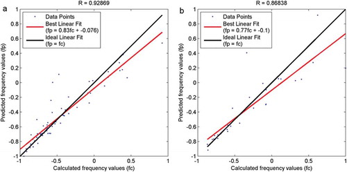
The results indicate that the functional relationship between the frequency of the first mode in cantilever beams as the dependent variable on one hand, and the beam length, the beam’s moment of inertia and the load applied on the beam as the independent variables on the other hand, can suitably be modeled using a feed-forward ANN trained by heuristic methods. Of the three heuristic methods tested, the ANN model trained using GA provided the best results. The ICA method had the best run time and came second in terms of accuracy. The best GA trained model was about 40% better than the best ICA trained model when comparing MSE on the training dataset, and about 6% better when comparing R² also on the training dataset. However, GA needs about 67% more time per possible solution per trial run of 1000 iterations. In order to improve the generalization properties of the ANN model, the heuristic algorithms needed to be slightly modified. In this paper, early stopping was implemented in all the three heuristic methods in order to improve generalization.

Conclusion

Determining the frequency of the first mode in the cantilever beams is complex and depends on several factors. Due to its complexity, estimating its value is difficult and is often carried out with a somewhat low accuracy.

In this paper, three parameters: the moment of inertia, beam loading, and beam length are selected as input or independent parameters, and the frequency of the first mode of cantilever beams is selected as the output or dependent parameter.

A feed-forward artificial neural network was used to model the relationship between these parameters. The neural network with an input layer of three neurons, two hidden layers each with five neurons and an output layer with one neuron (3–5-5–1) was deemed as suitable. Three different heuristic optimization methods were used to train the neural network model: genetic algorithm, PSO algorithm and imperialist competitive algorithm. The initial results of the training and test phases indicated that the heuristic algorithms needed to be slightly modified to include early stopping in order to improve the generalization capabilities of the neural network model. When the neural network model was trained using early stopping, model trained using GA outperformed the other models in terms of accuracy. The ICA trained neural network method came second in terms of accuracy but had the best run time. The best GA trained ANN model had an MSE value of 0.0110 and R² value of 0.9291 during the training phase with corresponding values of 0.0705 and 0.7013, respectively, for the test phase. The best ICA trained ANN model, on the other hand had an MSE value of 0.0198 and R² of value 0.8734 during the training phase with corresponding values of 0.0698 and 0.7132, respectively, for the test phase.

These results indicate the suitability of modeling the frequency of the first mode of cantilever beams using neural networks and training the neural network model using heuristic methods. Further research will be performed to determine a more suitable network structure, which would provide better prediction results.

Notes

^1. ICA was downloaded from: http://www.mathworks.com/matlabcentral/fileexchange/22046-imperialist-competitive-algorithm–ica-. PSO was downloaded from: http://www.particleswarm.info/SPSO2011_matlab.zip.

Both were accessed on January 7, 2015.

References

- Allen, D. E., and T. M. Murra. 1993. Design criterion for vibrations due to walking. Engineering Journal - American Institute of Steel Construction 117–29. Illinois.
- Alvis, S. R. 2001. An Experimental and Analytical Investigation of Floor Vibrations. Master’s Thesis, Faculty of the Virginia Polytechnic Institute and State University, April 2001, Blacksburg, Virginia.
- Atashpaz-Gargari, E., and C. Lucas. 2007. Imperialist competitive algorithm: An algorithm for optimization inspired by imperialistic competition. Proceedings of IEEE congress on evolutionary computation, September 25-28, Singapore, pp 4661–67.
- Atashpaz-Gargari, E., R. Rajabioun, F. Hashemzadeh, and F. L. Salmasi. 2009. A decentralized PID controller based on optimal shrinkage of Gershgorin bands and PID tuning using colonial competitive algorithm. International Journal of Innovative Computing, Information and Control (IJICIC) 5 10(A):3227–40.
- Bağdatlı, S. M., E. Özkaya, H. R. Özygit, and A. Tekin. 2009. Non-linear vibrations of stepped beam system using artificial neural networks. Structural Engineering and Mechanics 33 (1):15–30. doi:10.12989/sem.2009.33.1.015.
- Baker, J. E. 1987. Reducing bias and inefficiency in the selection algorithm, genetic algorithms and their applications. Proceedings of the Second International Conference on Genetic Algorithms (ICGA), Cambridge, Massachusetts, USA. July 28-31. pp 14–21.
- Beavers, T. A. 1998. Fundamental Natural Frequency of Steel Joist-Supported Floors. Master’s Thesis, Virginia Polytechnic Institute and State University, Blacksburg, Virginia.
- Behnia, A., H. K. Chai, N. Ranjbar, and N. Behnia. 2013. Finite element analysis of the dynamic response of composite floors subjected to walking induced vibrations. Advances in Structural Engineering 6 (5):959–74. doi:10.1260/1369-4332.16.5.959.
- Bishop, C. 2006. Pattern recognition and machine learning. Springer Science+Business Media, LLC, 233 Spring Street, New York, NY 10013, USA.
- Chen, M.-H., S.-H. Chen, and P.-C. Chang. 2015. Imperial competitive algorithm with policy learning for the traveling salesman proble. Soft Computing. doi:10.1007/s00500-015-1886-z.
- Clerc, M. 2012. Standard particle swarm optimisation, particle swarm central. Technical Report, Available online at: http://clerc.maurice.free.fr/pso/SPSOdescriptions.pdf, accessed 24 August 2014.
- CSA-Standard. 1999. Canadian standards association, guide for floor vibrations (steel structures for buildings-limit state design). CSA Standard CAN 3-S16, pp 1–89.
- Da Silva, J. G. S., P. C. :. G. Da S Vellasco, S. A. L. De Andrade, F. J. Da CPSoeiro, and R. N. Werneck. 2003. An evaluation of the dynamical performance of composite slabs. Computers and Structtures 81 (18–19):1905–13. doi:10.1016/S0045-7949(03)00210-4.
- Dash, T. 2015. A study on intrusion detection using neural networks trained with evolutionary algorithms. Soft Computing. doi:10.1007/s00500-015-1967-z.
- Ellis, B. R. 2001. Serviceability evaluation of floors induced by walking. The Structural Engineer 79 (21):30–36.
- Gerami, M., A. Sivandi Pour, and A. Dalvand. 2012. Determination of the natural frequency of the moment connections steel beams for controlling vibration of floors by artificial neural networks. Modares Civil Engineering Journal (M.C.E.L) 12 (2):113–25.
- Ghorban Pour, A. H., and M. Ghassemieh. 2009. Vertical vibration of composite floor by neural network analysis. Civil Engineering Infrastructures Journal (CEIJ) 43 (1):117–26.
- Goldberg, D. E. 1989. Genetic algorithms in search, optimization, and machine learning. Boston, MA, USA: Addison-Wesley Longman Publishing Co., Inc.
- Hadzima-Nyarko, M., D. Morić, H. Draganić, and E. K. Nyarko. 2012. New direction based (fundamental) periods of RC frames using genetic algorithms. Proceedings: 15WCEE, Lisboa, Portugal, No. 2493.
- Haykin, S. 1999. Neural networks: A comprehensive foundation, 2nd ed. Prentice Hall PTR Upper Saddle River, NJ, USA.
- Holland, J. H. 1992. Adaptation in natural and artificial systems: An introductory analysis with applications to biology, control, and artificial intelligence. Ann Arbor: The University of Michigan Press. 1975. Reprinted by MIT Press, April 1992, NetLibrary, Inc
- Housner, G. W. 1975. Dynamics of structures. R. W. Clough, and J. Penzien (eds.) New York: McGraw-Hill. wiley. doi:10.1002/eqe.4290040510
- Hudson, M. J., and P. Reynolds. 2012. Implementation considerations for active vibration control in the design of floor structures. Engineering Structures 44:334–58. doi:10.1016/j.engstruct.2012.05.034.
- Karlik, B., E. Özkaya, S. Aydin, and M. Pakdemirli. 1998. Vibrations of a beam-mass systems using artificial neural networks. Computers and Structures 69 (3):339–47. doi:10.1016/S0045-7949(98)00126-6.
- Kazemi, M. A., F. Nazari, M. Karimi, S. Baghalian, M. A. Rahbarikahjogh, and A. M. Khodabandelou. 2011. Detection of multiple cracks in beams using particle swarm optimization and artificial neural network. 4th International Conference on Modeling, Simulation and Applied Optimization (ICMSAO), Kuala Lumpur.
- Kennedy, J. 1999. Small worlds and mega-minds: Effects of neighborhood topology on particle swarm performance. Proceedings of the 1999 Congress on Evolutionary Computation, Washington, DC, USA, Vol. 3, p. 1938.
- Kennedy, J., and R. Eberhart. 1995. Particle swarm optimization. Proceedings of IEEE international conference on neural networks, pp 1942–48.
- Kennedy, J., R. Eberhart, and Y. Shi. 2001. Swarm intelligence. San Francisco, CA, USA.: Morgan Kaufmann Publishers Inc.
- Kennedy, J., and R. Mendes. 2002. Population structure and particle swarm performance. Proceedings of the 2002 Congress on Evolutionary Computation, CEC ’02, Honolulu, HI, USA, pp. 1671–76.
- Kuru, L., A. Ozturk, E. Kuru, and S. Cobanli. 2016. Active power loss minimization in electric power systems through chaotic artificial bee colony algorithm. Technical Gazzete 23 (2):491–98.
- Liang, J. J., A. K. Qin, P. N. Suganthan, and S. Baskar. 2006. Comprehensive learning particle swarm optimizer for global optimization of multimodal functions. IEEE T Evolut Comput 10 (3):281–95.
- Liu, L., X. Lai, K. Song, and D. Lao. 2015. Intelligent prediction model based on genetic algorithm and support vector machine for evaluation of mining-induced building damage. Tehnical Gazzete 22 (3):743–53.
- Marinaki, M., Y. Marinakis, and G. E. Stavroulakis. 2010. Vibration control of beams with piezoelectric sensors and actuators using particle swarm optimization. Expert System with Application 38 (6):6872–83. doi:10.1016/j.eswa.2010.12.037.
- Martell, J. L., A. Ebrahimpour, and M. P. Schoen. 2005. Intelligent approach to floor vibration control. Proceedings: ASME 2005 International Mechanical Engineering Congress and Exposition, Dynamic Systems and Control, Parts A and B, Orlando, Florida, USA. ISBN: 0-7918-4216-9.
- Middleton, C. J., and J. M. W. Brownjohn. 2010. Response of high frequency floors: A literature review. Engineering Structures 32:337–52. doi:10.1016/j.engstruct.2009.11.003.
- Morley, L. J., and T. M. Murray. 1993. Predicting floor response due to human activity. Proceedings of the IABSE International Colloquium on Structural Serviceability of Buildings, Gothenburg, Sweden, pp. 297–302.
- Murray, T. M., D. E. Allen, and E. E. Ungar. 1997. Steel design guide series 11: Floor vibrations due to human activity. Chicago, Illinois: American Institute of Steel Construction, Inc. (AISC).
- Nikoo, M., F. Ramezani, M. Hadzima-Nyarko, E. K. Nyarko, and M. Nikoo. 2016. Flood-routing modeling with neural network optimized by social-based algorithm. Natural Hazards. doi:10.1007/s11069-016-2176-5.
- Nikoo, M., F. Torabian Moghadam, and L. Sadowski. 2015. Prediction of concrete compressive strength by evolutionary artificial neural networks. Advances in Materials Science and Engineering. doi:10.1155/2015/849126.
- Özkaya, E., and M. Pakdemirli. 1999. Nonlinear vibrations of a beam-mass system with both ends clamped. Journal of Sound and Vibration 221 (3):491–503. doi:10.1006/jsvi.1998.2003.
- Przybylski, J. 2009. Non-linear vibrations of a beam with a pair of piezoceramic actuators. Engineering Structures 31 (11):2687–95. doi:10.1016/j.engstruct.2009.06.019.
- Ramezani, F., M. Nikoo, and M. Nikoo. 2015. Artificial neural network weights optimization based on social-based algorithm to realize sediment over the river. Soft Computing 19:375–87. doi:10.1007/s00500-014-1258-0.
- Sadowski, L., and M. Nikoo. 2014. Corrosion current density prediction in reinforced concrete by imperialist competitive algorithm. Neural Computing and Application 25:1627–38. doi:10.1007/s00521-014-1645-6.
- S-H., L., J.-G. Hsieh, J.-Y. Chang, and C.-T. Lin. 2015. Training neural networks via simplified hybrid algorithm mixing Nelder–Mead and particle swarm optimization methods. Soft Computing 19:679–89. doi:10.1007/s00500-014-1292-y.
- Sladki, M. J. 1999. Prediction of Floor Vibration Response using the Finite Element Method. Master’s Thesis, Faculty of the Virginia Polytechnic Institute and State University, Blacksburg, Virginia.
- Srinivas, M., and L. Patnaik. 1994. Adaptive probabilities of crossover and mutation in genetic algorithms. IEEE. T Syst Man Cyb 24 (4):656–67. doi:10.1109/21.286385.
- Waszczyszyn, Z., and L. Ziemiański. 2001. Neural networks in mechanics of structures and materials – new results and prospects of applications. Computers and Structures 79 (22–25):2261–76. doi:10.1016/S0045-7949(01)00083-9.
- Zambrano-Bigiarini, M., M. Clerc, and R. Rojas. 2013. Standard Particle Swarm Optimisation 2011 at CEC-2013: A baseline for future PSO improvements. IEEE Congress on Evolutionary Computation (CEC), Cancun, Mexico, pp. 2337–2344.