Mixed Biogeography-Based Optimization for GENCOs’ Maintenance Scheduling in Restructured Power Systems

ABSTRACT

Power industry restructuring has brought new challenges to the generation unit maintenance scheduling problem. Maintenance scheduling establishes the outage time scheduling of units in a particular time horizon. In the restructured power systems, the decision-making process is decentralized where each generating company (GENCO) tries to maximize its own benefit. Therefore, the principle to draw up the unit maintenance scheduling is different from the traditional centralized power systems. The objective function for GENCOs is to minimize his maintenance investment loss. Therefore, he hopes to put its maintenance on the weeks when the market-clearing price is lowest so that maintenance investment loss descends. This paper addresses the unit maintenance scheduling problem of GENCOs in restructured power systems. The problem is formulated as a mixed integer programming problem, and it is solved by using an optimization method known as biogeography-based optimization (BBO). BBO is simple to implement in practice and requires a reasonably small amount of computing time and a small amount of data communication. BBO has been tested by applying it to a GENCO with three generating units. This model consists of an objective function and related constraints, e.g., maintenance window, generation capacity, load and network flow. The simulation result of this method is compared with a classic method. The outcome is very encouraging and proves that BBO is powerful for minimizing GENCOs’ objective function.

Introduction

In restructured power systems, unit maintenance scheduling will not be decided only by the system dispatch center but will be mainly decided by generation companies (GENCOs). In this environment, GENCOs will try to schedule their units’ maintenance according to the operating conditions of their units, the quotations on the energy market and other economic factors. The goals of their unit maintenance schedule are to try to make their units have as long as possible life span and to make their power production earn as much as possible profit.

The power station maintenance department exists to help the production function to maximize plant reliability, availability and efficiency by determining both short- and long-term maintenance requirements and by carrying out the work accordingly. This includes work to comply with statutory and mandatory requirements and investigations into plant problems. The department has to make the most economic use of its available resources; this is achieved, in part, by having a level of staff (engineering, supervisory, craft) to deal with the general day-to-day steady workload and by making alternative arrangements to cater for work load peaks (Mohammadi Tabari, Pirmoradian, and Hassanpour 2008a).

To achieve the above goal, periodic servicing must take place and normally falls under the following items (Mohammadi Tabari, Pirmoradian, and Hassanpour 2008a):

1. Planned maintenance: overhaul, preventive maintenance

2. Unplanned maintenance: emergency maintenance

Preventive maintenance is expensive. It requires shop facilities, skilled labor, keeping records and stocking of replacement parts. However, the cost of downtime resulting from avoidable outages may amount to 10 or more times the actual cost of repair. The high cost of downtime makes it imperative to economic operation that maintenance be scheduled into the operating schedule (Mohammadi Tabari, Pirmoradian, and Hassanpour 2008a). The maintenance scheduling problem is to determine the period for which generating units of an electric power utility should be taken off line for planned preventive maintenance over the course of a 1 or 2-year planning horizon, in order to minimize the total operating cost while system energy, reliability requirements and a number of other constraints are satisfied (Marwali and Shahidehpour, 1998b).

Very recently, a new optimization concept, based on biogeography, has been proposed by Simon (Simon 2008). This new approach is known as biogeography-based optimization (BBO) (Ma and Simon 2011; Simon 2008, 2011a, 2011b). Biogeography is the study of the distribution of animals and plants over time and space. Its aim is to elucidate the reason of the changing distribution of all species in different environments over time. The environment of BBO corresponds to an archipelago, where every possible solution to the optimization problem is an island. Each solution feature is called a suitability index variable (SIV). The goodness of each solution is called its habitat suitability index (HSI), where a high HSI of an island means good performance on the optimization problem, and a low HSI means bad performance on the optimization problem. Improving the population is the way to solve problems in heuristic algorithms. The method to generate the next generation in BBO is by immigrating solution features to other islands and receiving solution features by emigration from other islands.

BBO has been applied to real-world optimization problems such as power system optimization (Bhattacharya and Chattopadhyay 2011; Rarick et al. 2009; Roy, Ghoshal, and Thakur 2010) and sensor selection (Simon 2008).

This paper solves a GENCO’s maintenance scheduling problem in the restructured power systems using BBO.

Solution approaches

Many efforts which are categorized as follows have been done in the maintenance scheduling field:

1. Ant colony optimization for continuous domains () (Fetanat and Shafipour, 2011a)

2. Harmony search algorithm (Fetanat and Shafipour, 2011b)

3. Quantum-inspired evolutionary algorithm (Fetanat et al. 2011)

4. Lagrangian relaxation (Geetha and Shanti Swarup 2009)

5. Particle swarm optimization (Siahkali and Vakilian 2009)

6. Implicit enumeration (Mohammadi Tabari, Pirmoradian, and Hassanpour 2008a)

7. Meta heuristic-based hybrid approaches (Dahal and Chakpitak 2007)

8. Ant colony optimization (Foong 2007)

9. Fuzzy logic (El-Sharkh, El-Keib, and Chen 2003; Huang, Lin, and Huang 1992; Leou 2001; Leou and Yih 2000)

10. Expert systems (El-Sharkh and El-Keib 2003; Lin et al. 1992)

11. Tabu search (El-Amin, Duffuaa, and Abbas 2000)

12. Simulated annealing (Daha et al. 2000)

13. Mixed integer programming (Da ilva, E. L, Schilling, M. T., & Rafael, M. C 2000)

14. Decomposition methods (Marwali and Shahidehpour, 2000a)

15. Goal programming (Moro and Ramos 1994)

16. Neural networks (Kim et al. 1999)

17. Linear programming (Chattopadhyay 1998)

18. Deterministic approaches (Marwali and Shahidehpour, 1998a)

19. Genetic algorithm (Barke and Smith 2000; Huang 1997, 1998; Wang and Handschin 2000)

Mixed integer programming problem

Problem contexts that involve both integer and continuous (real) decision variables are termed mixed integer programming.

Many real-world applications (e.g., airline crew scheduling, vehicle routing, production planning, etc.) require some variables to be integer. Some of the GENCOs’ maintenance scheduling problems are kind of mixed integer programming (Shahidehpour and Marwali 2000c).

In our proposed technique, integer variables are primarily released in the form of a real value. While running the algorithm, these variables which have to be changed into integer values are rounded to the closest integer value. In other words, suppose is the same real value that is supposed to be changed into integer value, so if , then is changed into ; otherwise, is changed into .

Method and formulations

We begin this section by presenting the general form of optimization problems. We then give the biogeography theory. Finally, we describe how the biogeography theory of the previous section can be applied to optimization problems.

General form

The optimization problem is specified as follows:

Minimize

Subject to

(1)

where is the objective function, is the number of inequality constraints and is the number of equality constraints. is the set of each decision variable and is the number of decision variables. The lower and upper bounds for each decision variable are and , respectively. Static penalty functions are used to calculate the penalty cost for an infeasible solution. The total cost for each solution vector is evaluated using

(2)

where and are the penalty coefficients. Generally, it is difficult to find a specific rule to determine the values of the penalty coefficients and normally these parameters remain problem dependent.

Biogeography

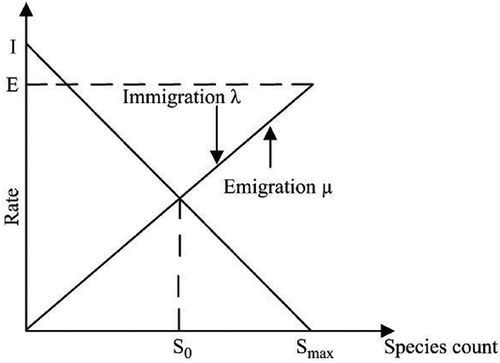
Biogeography describes how species migrate from one island to another, how new species arise and how species become extinct. A habitat is any island (area) that is geographically isolated from other islands. Areas that are well suited as residences for biological species are said to have a high HSI. Factors that influence HSI include rainfall, diversity of vegetation, topographic features, land area and temperature. The variables that characterize habitability are called SIVs. SIVs can be considered as the independent variables of the habitat, and HSI can be calculated using these variables. Habitats with a high HSI tend to have a large number of species, while those with a low HSI have a small number of species. Habitats with a high HSI have many species that migrate to nearby habitats, simply by virtue of the large number of species that they host. Migration of some species from one habitat to other habitat is known as emigration process. When some species enter into one habitat from any other outside habitat, it is known as immigration process. Habitats with a high HSI have a low species immigration rate because they are already nearly saturated with species. Therefore, high HSI habitats are more static in their species distribution than low HSI habitats. By the same token, high HSI habitats have a high emigration rate. Habitats with a low HSI have a high species immigration rate because of their sparse populations. This immigration of new species to low HSI habitats may raise the HSI of that habitat, because the suitability of a habitat is proportional to its biological diversity. Here, Figure 1 illustrates a model of species abundance in a single habitat. Let us consider the immigration graph of Figure 1. The maximum possible immigration rate to the habitat is , which occurs when there are zero species in the habitat. If a habitat has less number of species, then much larger amount of species from other habitat can enter into that habitat, so immigration rate is higher at that time. As the number of species increases, the habitat becomes more crowded, and fewer species are able to successfully survive after immigration to the habitat, and the immigration rate decreases. The largest possible number of species that the habitat can support is , at which point the immigration rate becomes zero, because no more species can enter into that habitat after that species count. Now consider the emigration graph. If there are no species in the habitat, then there is no species in that habitat that can shift to other habitat, so the emigration rate must be zero. As the number of species increases, the habitat becomes more crowded, more species are able to leave the habitat to explore other possible residences, and the emigration rate increases. The maximum emigration rate is , which occurs when number of species is . The equilibrium number of species is , at which point the immigration and emigration rates are equal. In Figure 1, immigration and emigration lines, graphically, have been shown as straight lines but, in general, they might be more complicated curves. However, the simple model gives us a general description of the process of immigration and emigration. In BBO algorithm, calculation of emigration rate and immigration rate is important as these play vital role to select habitats whose SIVs will undergo migration operation.

Figure 1. Species model of a single habitat.

Mathematically, the concept of emigration and immigration can be represented by a probabilistic model. Let us consider the probability that the habitat contains exactly species at . changes from time to time as follows (Simon 2008):

(3)

where and are the immigration and emigration rates when there are species in the habitat. This equation holds because in order to have species at time , one of the following conditions must hold (Simon 2008):

1. There were species at time , and no immigration or emigration occurred between and .

2. There were species at time , and one species immigrated.

3. There were species at time , and one species emigrated.

If time is small enough so that the probability of more than one immigration or emigration can be ignored, then taking the limit of Equation (3) as gives the following equation (Simon 2008).

(4)

From the straight-line graph of Figure 1, the equation for emigration rate and immigration rate for number of species can be written as per the following way (Simon 2008):

(5)

(6)

When value of , then combining Equations (5) and (6)

(7)

BBO

This section describes development of BBO technique and the different steps involved therein.

BBO concept is based on the two major steps, e.g., migration and mutation as discussed below.

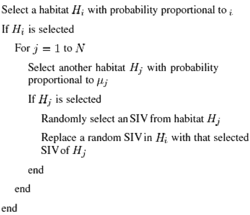
Migration

In BBO algorithm, a population of candidate solution can be represented as vectors of real numbers. Each real number in the array is considered as one (SIV). Using this SIV, the fitness of each set of candidate solution, i.e., HSI value, can be evaluated. In an optimization problem, high HSI solutions represent better quality solution, and low HSI solutions represent an inferior solution. The emigration and immigration rates of each solution are used to probabilistically share information between habitats. With probability , known as habitat modification probability, each solution can be modified based on other solutions. According to BBO if a given solution is selected for modification, then its immigration rate is used to probabilistically decide whether or not to modify each SIV in that solution. After selecting the SIV for modification, emigration rates of other solutions are used to select which solutions among the habitat set will migrate randomly chosen SIVs to the selected solution . In order to prevent the best solutions from being corrupted by immigration process, some kind of elitism is kept in BBO algorithm. Here, best habitat sets, i.e., those habitats whose HSI are best, are kept as it is without migration operation after each iteration. This operation is known as elitism operation (Simon 2008).

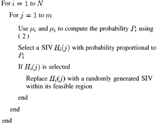
Mutation

It is well known that due to some natural calamities or other events, HSI of natural habitat might get changed suddenly. In BBO, such an event is represented by mutation of SIV and species count probabilities are used to determine mutation rates. The probabilities of each species count can be calculated using the differential equation of Equation (4). Each habitat member has an associated probability, which indicates the likelihood that it exists as a solution for a given problem. If the probability of a given solution is very low, then that solution is likely to mutate to some other solution. Similarly if the probability of some other solution is high, then that solution has very little chance to mutate. So, it can be said that very high HSI solution and very low HSI solutions have less chance to create more improved SIV in the later stage. But medium HSI solutions have better chance to create much better solutions after mutation operation. Mutation rate of each set of solution can be calculated in terms of species count probability using the following equation (Simon 2008):

(8)

where is a user-defined parameter and is the maximum . This mutation scheme tends to increase diversity among the habitats. Without this modification, the highly probable solutions will tend to be more dominant in the total habitat. This mutation approach makes both low and high HSI solutions likely to mutate, which gives a chance of improving both types of solutions in comparison to their earlier value. Few kind of elitism is kept in mutation process to save the features of a solution, so if a solution becomes inferior after mutation process, then previous solution (solution of that set before mutation) can be reverted back to that place again if needed.

BBO algorithm

The BBO algorithm can be described in the following way.

• Step 1) Initialize the BBO parameters like habitat modification probability , mutation probability, maximum mutation rate , max immigration rate , max emigration rate, lower bound and upper bound for immigration probability per gene, step size for numerical integration , number of habitat , number of SIV m, elitism parameter p which indicates the number of best habitats to be retained in the habitat matrix as it is, from one generation to the next without performing migration operations on them, etc. Set maximum number of iteration. Generate the SIVs of the given problem within their feasible region using random number. A complete solution consisting of SIVs is known as one habitat . There are several numbers of habitats to search the optimum result (Simon 2008).

• Step 2) Suppose we are minimizing a function that has been formulated as a mixed integer programming problem. Initialize several numbers of habitats depending upon the habitat size within feasible region. Each habitat represents a potential solution to the given problem. So, total habitat in matrix form is written in the following forms:

• Step 3) Calculate the HSI value for each habitat of the population set for given emigration rate and immigration rate . For the function , HSI of all SIV sets is calculated as per the following way:

Calculate the number of valid species out of all habitats using their HSI values. Those habitats, whose fitness values, i.e., HSI values, are finite, are considered as valid species .

• Step 4) Based on the optimum HSI value, elite habitats are identified.

• Step 5) Probabilistically, immigration rate and emigration rate are used to modify each non-elite habitat using migration operation. The probability that a habitat is modified is proportional to its immigration rate and the probability that the source of the modification comes from a habitat is proportional to the emigration rate . Habitat modification using migration operation can be described as Figure 2.

Figure 2. Habitat modification using migration operation.

From this algorithm, we note that elitism can be implemented by setting for the best habitats. After each habitat is modified, its feasibility as a problem solution should be verified. If it does not represent a feasible solution, then the above procedure is ignored and the same procedure is performed again in order to map it to the set of feasible solutions. After modification of each non-elite habitat using migration operation, each HSI is recomputed (Bhattacharya and Chattopadhyay, 2010; Simon 2008).

• Step 6) For each habitat, the species count probability is updated using Equation (4). Mutation operation is performed on each non-elite habitat and HSI value of each habitat is computed again. Figure 3 describes mutation operation.

Figure 3. Mutation operation.

As with habitat modification, elitism can be implemented by setting the probability of mutation selection to zero for the best habitats. After each habitat is modified, its feasibility as a problem solution should be verified. If it does not represent a feasible solution, then the above step is ignored and the abovementioned method is applied again in order to map it to the set of feasible solutions (Bhattacharya and Chattopadhyay, 2010; Simon 2008).

• Step 7) Go to step (3) for the next iteration. This loop can be terminated after a predefined number of iterations (generations) have been found.

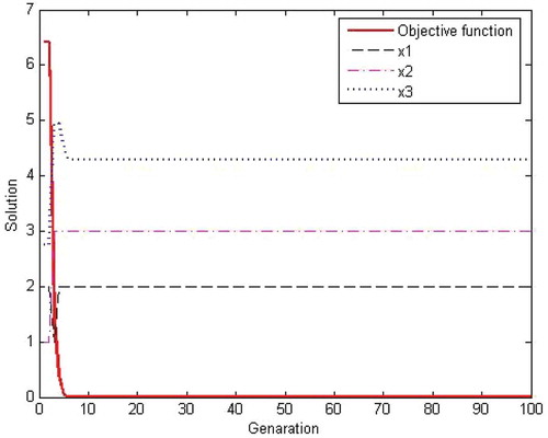
Finally, the values of calculated variables, respectively, are It is shown in Figure 4.

Figure 4. The value of calculated variables.

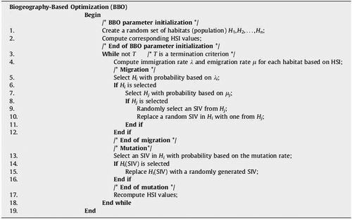
Figure 5 shows a pseudo code for BBO.

Figure 5. Pseudo code for biogeography-based optimization. Here, indicates habitat, HSI is fitness, SIV (suitability index variable) is a solution feature, denotes immigration rate and denotes emigration rate.

The GENCO’s maintenance model

The maintenance schedule determines periods when generating units in a GENCO are to be taken off line for planned preventive maintenance over the course of 1 year horizon (Marwali and Shahidehpour, 2000b). So that the loss of revenue is minimized while system energy, reliability as well as a number of other constraints are satisfied.

Objective function

Since the maintenance scheduling problem in a restructured power system becomes a multi-goal optimization problem, new model has to be sought to solve the maintenance schedule problem in restructured systems (Wang and Handschin 1999). The main purpose of a GENCO is making money as much as possible. As a matter of fact, the objective function is profit or the difference between total costs, which is the sum of different types of costs (such as maintenance cost of local transmission lines, maintenance cost and operation cost of generating units) and the income deriving from selling energy, as well. While we consider the income and also the costs in a 3-week period instead of the whole year, obviously the difference (on the other hand the profit) will be negative during this period of time, logically we use the term “loss of revenue” instead of profit, so minimizing the loss of revenue is the goal.

Constraints

Constraints may be categorized as coupling and decoupling constraints in time domain. The first set of coupling, or maintenance constraints, require that the units be overhauled regularly. This is necessary to keep their efficiency at a reasonable level, reduce force outage rates and prolong the life of the units. This procedure is incorporated periodicity by specifying min/max times that a generating unit may run without maintenance. The required time for overhauling a unit is generally given; hence, the number of weeks that a unit will be “down” is predetermined. It is assumed here that there is very little flexibility in the manpower usage and a limited number of units may be serviced at a given time. The available maintenance crew may categorize by location and responsibility. The availability of the crew in each category will be specified in the formulation (Marwali and Shahidehpour, 2000b). Network constraints in each time period are considered as decoupling constraints. The transportation model is adopted to represent system operation limits, peak load balance equation, generating and line capacity limits.

Mathematical description

The GENCO’s maintenance scheduling problem can be formulated as follows:

(9)

Subject to

Coupling constraints:

(10)

(11)

Decoupling constraints:

(12)

(13)

(14)

(15)

where

transmission maintenance cost/line in line at time .

generation maintenance cost for unit at time .

generation cost for unit at time .

number of circuits available in line at time , in the vector form is .

unit maintenance status, 0 if unit is offline for maintenance.

maximum number of circuits in line .

time period in which maintenance of generating unit starts.

forecast of market price at time .

earliest period for maintenance of generating unit to begin.

latest period for maintenance of generating unit to begin.

duration of maintenance for generating unit .

time period in which maintenance of line starts.

earliest period for maintenance of line to begin.

latest period for maintenance of line to begin.

duration of maintenance for line .

vector of dummy generators, which corresponds to energy not served at time period .

maximum generation capacity in vector form.

active power flow in vector form.

maximum generation capacity in vector form.

vector of, , power generating for each unit at time .

power generation of unit at time .

vector of demand in every bus at time .

node–branch incidence matrix.

maximum power generation of unit .

minimum power generation of unit .

The unknown variables and in the all abovementioned equations are restricted to integer values; on the other hand, and have continuous values. The objective of Equation (9) is to minimize the loss of revenue over the operational planning period. The first term of the objective function Equation (9) is the maintenance cost of generators, the second is transmission line maintenance cost, the third is the energy production cost and the fourth is the income from selling produced energy over the planning period.

Constraints Equation (10) represent the maintenance window stated in terms of the start of maintenance variables . The unit and the line must be available both before their earliest period of maintenance and their latest period of maintenance, e.g., . Set of constraints Equation (11) consists of crew and resource availability, seasonal limitation and desirable schedule. The seasonal limitation can be incorporated into and values of constraint Equation (10). If we consider for example that lines 1, 2 and 3 are to be maintained simultaneously, the set of constraints can be formed as follows:

If the GENCOs have limited crew and resources available for maintenance, it assumed that in each time interval (e.g., 1 week) we can put only one generating unit and one local transmission line off-line simultaneously for yearly maintenance program. Constraints Equations (12)–(15) represent peak load balance and other operational constraints such as generation and transmission capacity limits (Marwali and Shahidehpour, 1998a, 1999; Mohammadi Tabari, Pirmoradian, and Hassanpour 2008b; Shahidehpour and Marwali 2000c).

Case study

This paper introduces a GENCO with three generating units and three double circuit transmission lines. For convenience, in this study, all lines are assumed to be perfectly reliable. The specifications of GENCO’s generators, transmission lines and load are given in Tables 1–3. The problem is defined as follows: the GENCO wants to perform maintenance on one generator and one transmission line in each step of the study period due to limited number of crew and resources and also the low market price of electricity on that specific 3-week study period, which consists of three 1 week time interval. The main factor for scheduling in a competitive environment is the amount of electricity that a GENCO sell. The market price forecast, for the whole 3-week planning period, is shown in Table 4 (Mohammadi Tabari, Pirmoradian, and Hassanpour 2008b).

Table 1. GENCO’s generators specification.

Unit No.	Min. capacity, (p.u.)	Max. capacity, (p.u.)	Operation cost ($)	Maintenance cost ($/p.u.)
1	0.5	2.5		300
2	0.6	2.5		200
3	0.6	2.5		100

Table 2. GENCO’s transmission lines specification.

Line No.	Buses of line	No. of circuits	Maintenance cost ($/line)	Max. capacity/circuit (p.u.)
1	1–2	2	100	0.5
2	2–3	2	200	1
3	1–3	2	300	0.5

Table 3. Load specification.

Bus No.	Load (p.u.)	Generator
1	1
2	3
3	1

Table 4. The market price forecast.

Week No.	Average market price forecast ($)
1	55
2	50
3	45

Putting the above data in the formulation of previous section, we will come to the following mathematical model:

Objective function:

Subject to

Numerical results

In order to verify BBO can supply an optimal unit maintenance schedule, a GENCO that must be maintained during a 3-week period was adopted as the test system. Programming commands used in this simulation are taken from MATLAB. In Equation (2), and are 10,000. The obtained results are shown in Table 5. This table shows that in the first week, the third generator and the second line should be maintained. In the second week, the first generator and the first line is put off line. Finally, the second unit and the third line must be serviced during the third week.

Table 5. The value of maintenance variables.

Maintenance variables
	1		2		2.5		0
	0		0		0		1
	1		2		2.0846		0
	1		0		2.4343		0.5799
	1		2		2.5		0
	0		2		0		2
	0		2		0		1
	1		2		2.5		0
	1		0		3		0

Also, the minimum value of loss of revenue is $1200. Figure 6 shows the convergence of BBO.

Figure 6. The convergence of BBO for the GENCO model.

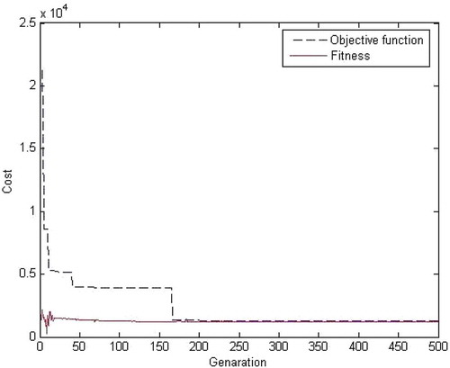
Compared with branch-and-bound optimization method that calculates Z in 1200 value (Mohammadi Tabari, Pirmoradian, and Hassanpour 2008b), BBO is more accurate and also has the greater velocity.

Conclusion

This paper introduces BBO to optimize the unit maintenance scheduling of GENCOs in restructured power systems. A GENCO’s maintenance scheduling problem (as a mixed integer programming problem) has been solved. BBO gives optimal maintenance schedule. All the constraints are satisfied. The obtained result using BBO in Table 5 has been compared with branch-and-bound optimization method. The result reveals that BBO outperforms this classic method in terms of reaching an effective solution and fast convergence. Also, the proposed method has a high degree of flexibility. Therefore, it is easier to implement. Finally, this paper demonstrates with clarity successful application of BBO to GENCOs’ maintenance scheduling.

References

- Arun, N., and V. Ravi. 2009. ACONM: A hybrid of ant colony optimization and nelder-mead simplex search. India: Institute for Development and Research in Banking Technology (IDRBT).
- Barke, E. K., and A. J. Smith. 2000. Hybrid evolutionary techniques for the maintenance scheduling problem. IEEE Transactions on Power Systems 15:122–28.
- Bhattacharya, A., and P. Chattopadhyay. 2010. Solving complex economic load dispatch problems using biogeography-based optimization. Expert Systems with Applications 37:3605–15.
- Bhattacharya, A., and P. Chattopadhyay. 2011. Hybrid differential evolution with biogeography-based optimization algorithm for solution of economic emission load dispatch problems. Expert Systems with Applications 38:14001–10.
- Bosman, P. A. N., and D. Thierens. 2002. Continuous iterated density estimation evolutionary algorithms within the IDEA framework. In Proceedings of OBUPM workshop at GECCO-2000, eds. M. Pelikan, H. Mü Hlenbein, and A. O. Rodriguez, 197–200. San Francisco, CA: Morgan-Kaufmann Publishers.
- Chattopadhyay, D. A. 1998. Practical maintenance scheduling program: Mathematical model and case study. IEEE Transactions on Power Systems 13:1475–80.
- Da ilva, E. L., Schilling, M. T., and Rafael, M. C. 2000. Generation maintenance scheduling considering transmission constraints. IEEE Transactions on Power Systems 15:838–43.
- Daha, K. P., G. M. Burt, J. R. McDonald, and S. J. Galloway (2000). Ga/sa based hybrid techniques for the scheduling of generator maintenance in power systems. In Proceedings of Congress on Evolutionary Computation, La Jolla, CA, USA, July 16–19, pp. 547–567.
- Dahal, K. P., and N. Chakpitak. 2007. Generator maintenance scheduling in power systems using meta heuristic-based hybrid approaches. Electric Power Systems Research Journal 77:771–79.
- El-Amin, I., S. Duffuaa, and M. Abbas. 2000. A Tabu search algorithm for maintenance scheduling of generating units. Electric Power Systems Research 54:91–99.
- El-Sharkh, M. Y., and A. A. El-Keib. 2003. An evolutionary programming-based solution methodology for power generation and transmission maintenance scheduling. Electric Power Systems Research Journal 65:35–40.
- El-Sharkh, M. Y., A. A. El-Keib, and H. Chen. 2003. A fuzzy evolutionary programming-based solution methodology for security-constrained generation maintenance scheduling. Electric Power Systems Research 67:67–72.
- Fetanat, A., and G. Shafipour. 2011a. Generation maintenance scheduling in power systems using ant colony optimization for continuous domains based 0-1 integer programming. Expert Systems with Applications 38:9729–35.
- Fetanat, A., and G. Shafipour. 2011b. Harmony search algorithm based 0-1 integer programming for generation maintenance scheduling in power systems. Journal of Theoretical and Applied Information Technology 24:1–10.
- Fetanat, A., G. Shafipour, M. Yavandhasani, and F. Ghanatir. 2011. Optimizing maintenance scheduling of generating units in electric power systems using quantum-inspired evolutionary algorithm based 0-1 integer programming. European Journal of Scientific Research 55:220–31.
- Foong, W. K. 2007. Ant colony optimization for power plant maintenance scheduling. PhD thesis, The University of Adelaide.
- Geetha, T., and K. Shanti Swarup. 2009. Coordinated preventive maintenance scheduling of GENCO and TRANSCO in restructured power systems. International Journal of Electrical Power & Energy Systems 31:626–38.
- Huang, C. J., C. E. Lin, and C. L. Huang. 1992. Fuzzy approach for generator maintenance scheduling. Electric Power Systems Research 24:31–38.
- Huang, S. 1997. Generator maintenance scheduling: A fuzzy system approach with genetic enhancement. Electric Power Systems Research Journal 41:233–39.
- Huang, S. 1998. Genetic-evolved fuzzy system for maintenance scheduling of generating units. Electrical Power and Energy Systems 20:191–95.
- Kim, H., S. Moon, J. Choi, S. Lee, D. Do, and M. M. Gupta (1999). Generation maintenance scheduling considering air pollution based on the fuzzy theory. In Proceedings of IEEE International Fuzzy System, Seoul, Korea, August 22–25, pp. III-1759–III-64.
- Leou, R. C. 2001. A flexible unit maintenance scheduling considering uncertainties. IEEE Transactions on Power Systems 16:552–59.
- Leou, R. C., and S. A. Yih (2000). A flexible unit maintenance scheduling using fuzzy 0–1 integer programming. In Proceedings of IEEE Power Engineering Society Summer Meeting, Seattle, WA, USA, July 16–20, pp. 2551–2555.
- Lin, C. E., C. J. Huang, C. L. Huang, C. C. Liang, and S. Y. Lee. 1992. An expert system for generator maintenance scheduling using operation index. IEEE Transactions on Power Systems 7:1141–48.
- Ma, H., and D. Simon. 2011. Analysis of migration models of biogeography-based optimization using Markov theory. Engineering Applications of Artificial Intelligence 24:1052–60.
- Marwali, M. K. C., and S. M. Shahidehpour. 1998a. Integrated generation and transmission maintenance scheduling with network constraints. IEEE Transactions on Power Systems 13:1063–68.
- Marwali, M. K. C., and S. M. Shahidehpour. 1998b. A deterministic approach to generation and transmission maintenance scheduling with network constraints. Electric Power Systems Research Journal 47:101–13.
- Marwali, M. K. C., and S. M. Shahidehpour. 1999. Long-term transmission and generation maintenance scheduling with network, fuel, and emission constraints. IEEE Transactions on Power Systems 14:1160–65.
- Marwali, M. K. C., and S. M. Shahidehpour. 2000a. Short-term transmission line maintenance scheduling in a deregulated system. IEEE Transactions on Power Systems 15:1117–24.
- Marwali, M. K. C., and S. M. Shahidehpour. 2000b. Coordination between long-term and short-term generation scheduling with network constraints. IEEE Transactions on Power Systems 15:1161–67.
- Mohammadi Tabari, N., M. Pirmoradian, and S. B. Hassanpour (2008a). Implicit enumeration based 0–1 integer programming for generation maintenance scheduling. In Proceedings of the International Conference on Computational Technologies in Electrical and Electronics Engineering (IEEE REGION 8 SIBIRCON 2008), Novosibirsk, Russia, July 21–25, pp. 151–154.
- Mohammadi Tabari, N., M. Pirmoradian, and S. B. Hassanpour (2008b). Revenue based maintenance scheduling of a GENCO in restructured power systems. In Proceedings of 5th International Conference on Electrical Engineering/Electronics, Computer, Telecommunications and Information Technology, Krabi, Thailand, May 14–17, pp. 873–876.
- Moro, L. M., and A. Ramos. 1994. Goal programming approach to maintenance scheduling of generating units in large scale power systems. IEEE Transactions on Power Systems 14:1021–28.
- Rarick, R., D. Simon, F. E. Villaseca, and B. Vyakaranam (2009). Biogeography-based optimization and the solution of the power flow problem. In Proceedings of the IEEE Conference on Systems, Man, and Cybernetics, San Antonio, Texas, October 11–14, pp. 1029–1034.
- Roy, P., S. Ghoshal, and S. Thakur. 2010. Biogeography based optimization for multi-constraint optimal power flow with emission and non-smooth cost function. Expert Systems with Applications 37:8221–28.
- Shahidehpour, S. M., and M. K. C. Marwali. 2000c. Maintenance scheduling in restructured power systems, 1st ed. ed. Norwell, MA: Kluwer.
- Siahkali, H., and M. Vakilian. 2009. Electricity generation scheduling with large-scale wind farms using particle swarm optimization. Electric Power Systems Research Journal 79:826–36.
- Simon, D. 2008. Biogeography-based optimization. IEEE Transactions on Evolutionary Computation 12:702–13.
- Simon, D. 2011a. a. in print: A dynamic system model of biogeography-based optimization. Applied Soft Computing.
- Simon, D. 2011b. b. A probabilistic analysis of a simplified biogeography-based optimization algorithm. Evolutionary Computation 19:167–88.
- Wang, Y., and E. Handschin (1999). Unit maintenance scheduling in open systems using genetic algorithm. In Proceedings of IEEE Transmission and Distribution Conference, New Orleans, LA, USA, April 11–16, pp 334–39.
- Wang, Y., and E. Handschin. 2000. A new genetic algorithm for preventive unit maintenance scheduling of power systems. Electrical Power and Energy Systems 22:343–48.