A Comparative Study of Classical Clustering Method and Cuckoo Search Approach for Satellite Image Clustering: Application to Water Body Extraction

ABSTRACT

Image clustering is a critical and essential component of image analysis to several fields and could be considered as an optimization problem. Cuckoo Search (CS) algorithm is an optimization algorithm that simulates the aggressive reproduction strategy of some cuckoo species.

In this paper, a combination of CS and classical algorithms (KM, FCM, and KHM) is proposed for unsupervised satellite image classification. Comparisons with classical algorithms and also with CS are performed using three cluster validity indices namely DB, XB, and WB on synthetic and real data sets. Experimental results confirm the effectiveness of the proposed approach.

Introduction

Nowadays, remote-sensing images are acquired more frequently, quickly and contained much additional information than last years. Also, these images are used in different areas, such as mapping land-use and land-cover, agriculture, forestry, urban planning, military observation, change detection, vegetation health, and water resource investigations (Campbell 2002). For all these applications it is very important and crucial to extract pertinent information automatically by applying different steps: data preprocessing, feature reduction, image analysis. This latter includes classification step which is considered as a very important task in remote sensing, and aims to partition pixels in the images into homogeneous regions, each pixel corresponds to some particular landcover type (Bandyopadhyay, Maulik, and Mukhopadhyay 2007). In classification image, a distinction is often made between supervised and unsupervised methods. Labeled training samples are required by supervised algorithms to perform the classification: it is frequently the analyst who gives these data. By contrast, the unsupervised classification needs fewer data from the analyst; the most necessary one is the image regions’ number (Ming-Der 2007). Classification image can be viewed as a clustering problem in the space intensity (Maulik and Bandyopadhyay 2003), and thus several clustering algorithms have been used to resolve it (Tong et al. 2009).

The aim of clustering is to find the optimal partition of a specified n data points into c subgroups, such that the inter-class distance is as far as possible whereas the intra-class distance is as close as possible (Swagatam and Amit 2009). The assignment of a data to a group could be done in two different manners: The first one allows one piece of data to belong to two or more clusters with some probabilities, while the second one assumes that each data belongs to only one cluster. These approaches are known in literature as Fuzzy (Soft) and Hard (Crisp) clustering, respectively. Also, conventional (classical) clustering algorithms can be divided into two categories: hierarchical clustering and partitional clustering (Zhao 2012). A hierarchy of clusters could be constructed in a divisive way (a large cluster is split into smaller ones) or agglomerative way (smaller clusters are merged to obtain larger ones) by hierarchical algorithms (Gan, Ma, and Wu 2007, Zhao 2012). Partitional algorithms relocate iteratively data points between clusters in order to minimize certain criteria and have an optimal partition. For remote-sensing image, hierarchical methods are not very adopted because of the large used data sets which caused a big memory space and CPU time. However, partitional methods are very used, but have two principal drawbacks: initial number of clusters and its convergence to local optimal. Isodata, Fuzzy C-means (FCM), KMeans (KM), and its variant K-Harmonic Means (KHM) are considered as the most popular partitional methods in remote-sensing images. On another hand, and in order to avoid disadvantages of classical algorithms, scientists used new methods based on bio-inspired algorithms (BIAs). These latter are inspired from the behavior observed in biological systems which learn naturally how to adjust to changes automatically; they are robust, flexible, and evolving (Khalid et al. 2011). In remote sensing, BIAs algorithms are generally used as clustering-based methods (Tong, Man, and Xiang 2009).

Furthermore, different validity criteria have been developed to evaluate and compare clustering algorithms results. They can be used, in addition, to determine the optimal clusters number in a data set. Usually, three groups are distinguished in cluster validity techniques: internal, external, and relative. For the two first approaches, expensive computational statistical tests are needed. For the third approach, the choice of the best clustering result out of a set of defined schemes is attributed to a predefined criterion. There are some authors in the literature who classify cluster validity techniques into only two groups: internal and external. Working with cluster validation techniques deal to implement numerical measures known as cluster validity indices (CVI). There are fuzzy and crisp indices, Xie-Benie (XB) index (Xie and Beni 1991) as well as Bezdek’s PE and PC indices (Bezdek 1974) (Bezdek 1975) which are some examples of the first category. Concerning Davies-Bouldin (DB) index (Davies and Bouldin 1979), Dunn’s index (Dunn 1974), Calinski-Harabasz index (Calinski and Harabasz 1973), and recently Sum-of-squares-based validity index called WB index (Zhao and Fränti 2014) are some of the most popular indices used in the second category. Pakhira, Bandyopadhyay, and Maulik 2005, Arbelaitz et al. 2013 and Halkidi, Batistakis, and Vazirgiannis 2002 give a very important review of different CVIs present in the literature.

There is an intensive research using BIAs algorithms, as Genetic Algorithms (GA), Particle Swarm Optimization (PSO), Artificial Immune System (AIS), Artificial Bee Colony (ABC), and Neural Networks (NN) (Khalid et al. 2011, Costa and De Souza 2011). We also find efficient hybrid optimization algorithms and multi-objective algorithms (Bong and Rajeswari 2011). Cuckoo Search Algorithm (CSA) (Yang 2010) is one of the recent BIAs which prove their efficiency and have been applied in several optimization and computational intelligence. Many other works attempted to improve CSA, like Walton et al. (2011), Valion et al. (2011), and Tuba, Subotic, and Stanarevic (2012). The reader interested in recent CSA advances and applications can refer to Yang and Deb (2014) and Azizah, Azlan, and Nor (2014). CS has been employed as a clustering algorithm in different works such as Saida, Nadjet, and Omar (2014), Senthilnath et al. (2013), Manikandan and Selvarajan (2014), Goel, Sharma, and Bedi (2011), and Zhao et al. (2014).

In BIAs, CVI can be used as a fitness function to optimize or as a measure to evaluate the quality of the result. In remote-sensing clustering problems, a lot of CVIs have been developed and tested (Pakhira, Bandyopadhyay, and Maulik 2005), and this makes the choice of the most suitable index for a bio-inspired method difficult. In this study, the CS algorithm is employed for unsupervised satellite image classification. A new approach based on the combination of Cuckoo Search (CS) and classical algorithms (KM, FCM, and KHM) is proposed for unsupervised satellite image classification. This combination, named CSC, uses as initial population a combination between random solutions and the best solutions provided by the classical algorithms. The motivation is to guide the search of CS toward good solutions, with the aim to assure a fast convergence and to avoid local optimal. This approach is compared with classical algorithms and also with CS using a random initial population. In addition, in both bio-inspired approaches, CS and CSC, three CVIs namely XB, DB, and WB are used as fitness functions, in order to study the performance of methods for different indices and choose the best one to use in conjunction with them. Further, water body extraction is used in this work as an application of clustering problem. In fact, a great deal of research over the last years has been conducted to extract water body from various multi-resolution remote-sensing images issue from different satellites (Spot, LandSat, etc.). Water body extraction is important for the prediction, monitoring of flood disasters, and water planning with accurate effectiveness (Li et al. 2011, Haibo et al. 2011).

This paper is organized as follows. A brief introduction about clustering algorithms used in this work is given in Section “Clustering algorithms”. The methodology of CS and its adaptation for clustering problem is described in Section “Methodology”. Experimental results on both synthetic and real data sets are given in Section “Experimental results”. Conclusions and future work are drawn in Section “Conclusion”.

Clustering algorithms

This section presents a brief description of the classical clustering algorithm KHM employed in this paper for comparison. For a more detailed description about classical clustering algorithms used in this work namely K-Means, FCM, interested readers are referred to MacQueen (1967), Bezdeck (1984), and Zexuan et al. (2012).

In the next sections, the following notation will be adopted:

N: number of items to be clustered in the data set X, K: number of clusters, c_j: jth cluster center, x_i: ith data set item.

KHM algorithm

The main drawback of K-Means algorithm is the dependence of its performance on the initialization of centers. To improve the algorithm, Zhang (2000) proposes to use the harmonic mean instead of standard mean in the objective function and has named the new algorithm KHM.

(1)

New centers clusters are calculated as following (Zhang et al. 2013, Thangavel and Karthikeyani Visalakshi 2009):

(2)

Methodology

This section presents the concepts of CSA and explains how its integration and application for solving clustering problem is carried out.

Cuckoo behavior

CSA is a nature-inspired technique for solving nonlinear optimization problems. It has been developed by Yang and Deb in 2009, and the preliminary studies show that it is very promising and could outperform existing algorithms, such as GA and PSO (Yang 2010). This algorithm is based on the aggressive reproduction strategy of some cuckoo species in combination with Lèvy flight behavior of some birds and fruit flies (Yang and Deb 2009, Reynolds and Frye 2007).

In reality, a lot of species of cuckoo exist; some of them use communal nests to lay their eggs. However, cuckoos may remove other birds’ eggs in order to increase the hatching probability of their eggs. Some other cuckoo species use the nests of other host birds (often other species) to lay their eggs. When a host bird discovers that the eggs are not its own, it will either abandon its nest and build another new one elsewhere or throw these alien eggs away. Also, there are some other cuckoo species which have female parasitic cuckoos very specialized in mimicking a few chosen host species in color and pattern of host eggs. In this way, the cuckoos diminish the possibilities of abandoning their eggs and therefore improve their reproductivity (Payne, Sorenson, and Klitz 2005).

The random process which takes a series of consecutive random steps is called a random walk. In nature, the search of food by animals is operated in a random or quasi-random manner and can be considered as a random walk. In fact, the next move in an animal foraging path is based on the current location/state and the transition probability to the next location. The chosen direction implicitly depends on a probability, which can be modeled mathematically (Yang 2010). A Lèvy flight is a random walk in which step lengths are drawn according to a heavy-tailed probability distribution (Gandomi, Yang, and Alavi 2013). Yang and Deb (2009) have employed this behavior in CSA to assure local search and exploration phase.

Cuckoo Search Algorithm

Yang and Deb (2009) have used the following three rules which aim at applying CSA, an optimization tool, and simplifying this tool description:

• One egg is, at a time, laid by each cuckoo and dumped (its egg) in a nest randomly selected.

• The best solutions will carry on over to the next generations by using the elitist selection.

• The number of host nests is predetermined, and a host bird can discover an egg laid by a cuckoo with a probability P_a.

In this case, the host bird can either throw the alien egg away or desert the nest so as to make a new nest in another location. For simplicity, this last assumption can be verified by a fraction P_a of the n nests being replaced by new random solutions at new locations.

Yang and Deb (2009) assume that each egg in a nest represents a solution, and a cuckoo’s egg represents a new solution. The aim is to replace bad solutions (cuckoos) in the nests by new and potentially better solutions.

Algorithm 1 summarizes the pseudo code of the basic steps of CS based on the above rules.

Algorithm 1 Original Cuckoo Search (Yang 2010)

1: Generate initial population of n host nests x_i;

2: Loop

3:     Get a cuckoo randomly by Lévy flight and evaluate its quality/fitness F_i;

4:    Choose a nest among n (say, j) randomly;

3:    If (F_i > F_j), replace j by the new solution;

4:      A fraction (P_a) of worse nests are abandoned and new ones are built;

5:     Keep the best solutions (or nests with quality solutions);

6:     Rank the solutions and find the current best;

7:  If a criterion is met (usually a sufficiently good fitness or a maximum number of iterations), exit loop

8: End loop

9: Post process results and visualization.

For generating new solutions x_i(t + 1), a local random walk (Equation 3) and global random walk by using Lèvy flights (Equation 4) are performed. Mathematically speaking, the random walk is given by the following equation:

(3)

where x is the current solution at t, and w_t is a step or a random variable with a known distribution (Yang 2010). In the real world, the probability of discovering cuckoos’ eggs depends on its similarity with the hosts’ eggs. It means that the former which is different from the latter has a big probability to be discovered. To modelize this situation, Yang (2010) choose a random walk in biased way with some random step sizes in order to relate the difference in solutions with fitness. For generating new solutions x_i(t + 1), a Lévy flight is performed as follows: (Yang 2010):

(4)

where α > 0 is the step size which should be related to the scales of the problem under consideration. The product Å means entry-wise multiplications. The Lèvy flights essentially provide a random walk, while their random steps are drawn from a Lévy distribution for large steps which has an infinite variance and mean.

Here, the successive jumps of a cuckoo form a random walk process which obeys a power-law step-length distribution with a heavy tail.

(5)

Current approach

CSA has been used in this work to determine the centers of clusters for unsupervised satellite image classification. The proposed approach is described in detail within the following sections, including solutions codification and fitness function.

Coding

In a clustering problem, the data set is composed of N objects, each one of them is defined by l attributes. In order to resolve clustering problem, the CS algorithm is adopted to find K cluster centers from the data set by optimizing a fitness function.

In CS mechanism, the nests represent the solutions. Hence, each nest in this work is a set of K centers and can be represented by a matrix K × l, where l represents the number of attributes of each center.

Fitness function

In this paper, three popular clustering validity indices –DB, XB, and WB – are used as an objective function (Fitness) which needs to be optimized. Next, the equations of CVI are given.

The DB index

It is a very popular and used crisp index in clustering algorithms. It is defined by Davies and Bouldin (DB) (Davies and Bouldin 1979) and requires only two parameters to be defined by the user – p (distance measure) and q (dispersion measure). The DB index is defined as follows:

(6)

with

(7)

(8)

where c_ki : kth component of the n-dimensional vector c_i, c_i : the center of cluster i, M_ij : the Minkowski metric, and T_i : the number of vectors in cluster i.

Xie-Beni (XB) index

The XB index (called also function S) is defined as a function of the ratio of the total variation to the minimum Separation of clusters (Xie and Beni 1991):

(9)

Sum-of-squares based validity index (WB)

WB index (WB) (Zhao. et al. 2014) is defined as a ration of the measure of compactness of the cluster to its measure of separation. It is given by

(10)

where

c_Pi: the center of the cluster P_i to which belongs the element x_i, /N is the mean value of the whole data set and is the number of elements in each cluster.

Algorithm

The clustering CS algorithm adopted in this work follows the above steps.

Algorithm 2 Clustering Cuckoo Search

1. Generate initial population of nb_nest host nests;

2. Evaluate the fitness of each solution Fit_old and select the best solution: best_nest;

Loop

3. Generate nb_nest-1 new solutions by the cuckoo search lèvy flight except for the best_nest (Exploration phase);

4. Evaluate the fitness of the new solutions Fit_new;

5. For each solution, if Fit_new < Fit_old, replace the old nest by the new one;

6. Generate a fraction (P_a) of new solutions to replace the worse nests (Exploitation phase);

7. Compare these solutions with the old solutions. If Fit_new < Fit_old, replace the old nest by the new one;

8. Find the best solution best_nest;

9: If a criterion is met (usually a sufficiently good fitness or a maximum number of iterations), exit loop

10. End loop

11. Post process results and visualization.

Experimental results

In this section, the used data sets, experimental results, and discussions about findings performance will be given. Three subsections are supplied; the first will present different data sets used in this work. The second subsection will explain experimental results on synthetic data sets. Results with real data sets are given in the third subsection. Three classical methods are used to compare with CS namely: FCM, KM, and KHMeans. All results concerning CS and CSC are done with two values of the step size α (0.01 and 0.1). In the rest of the paper, the CS with α = 0.01 is noted CS1 (respectively CSC1) and CS2 (respectively CSC2) for CS with α = 0.1.

All computations have been done using MATLAB programming language on an Intel Pentium Dual-Core with 2.13 GHZ CPU and 4 GB of RAM. Experiments were conducted to demonstrate the efficiency of the methodology using synthetic and real data sets.

Data sets

Synthetic data sets used in this work namely S1 and S2 (Figure 1(a), (b)) have been generated using Gaussian distribution and can be found in the SIPU web page http://cs.uef.fi/sipu/datasets.

Figure 1. Synthetic data S1 (a) and S2 (b) (from left to right).

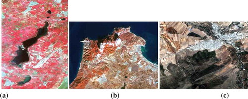
The second set of experimentations is performed on three multispectral remotely sensed data which present more complexity than the first set of experimentations used earlier. The first real data set consists of three multispectral Spot 5 bands with spatial resolution of 10 m and window size of 800 × 1500 pixels representing the region of Oran (West of Algeria) as illustrated in Figure 2(a). Landsat 8 image sub-scene of Arzew, with three spectral data channels, size of 800 × 600, and a spatial resolution of 30 m is used as second data set and shown in Figure 2(b). The last remote sensed data is obtained from Alsat-2A image of a part of the city of Tlemcen 500 × 500 (West of Algeria) and shown in Figure 2(c). The characteristics of each image are given in Table 1.

Table 1. The characteristics of images.

Satellite	Bands	Wavelength	Acquisition date
Spot 5	Band1: Green Band2: Red Band3: Near-infrared (NIR)	0.50–0.59 µm 0.61–0.68 µm 0.78–0.89 µm	March 3, 2012
Landsat-8 Enhanced Thematic Mapper Plus (ETM+)	Band2: Green Band4: Red Band5: Near-infrared (NIR)	0.525–0.605 µm 0.63–0.69 µm 0.75–0.90 µm	May 4, 2014
Alsat-2A	Band2: Green Band3: Red Band4:Near-infrared (NIR)	0.53–0.59 µm 0.62–0.69 µm 0.76–0.89 µm	May 4, 2011

Figure 2. Real images used for experimentations.

Synthetic data results

In order to analyze the performance of all methods used in this work (FCM, KMeans, KHMeans, CS and CSC) based one, experiments varying the number of clusters from K = 10 to K = 20 have been carried out. The values of validity indices on DB index, XB index, and WB index with all the methods for S1 data set are plotted as shown in Figures 3, 4, and 5, respectively.

Figure 3. Variation of the DB index with respect to the number of clusters for the S1 data set with all methods.

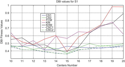
Figure 4. Variation of the XB index with respect to the number of clusters for the S1 data set with all methods.

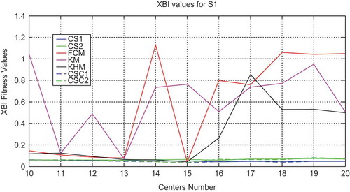
Figure 5. Variation of the DB index with respect to the number of clusters for the S1 data set with all methods.

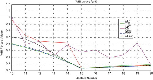
As shown in Figure 3 and Figure 4, values of indices have higher variance with the classical algorithms (FCM, KM, and KHM) than CS and CSC algorithms for DB and XB indices. Concerning WB index, all the algorithms present less variance from K = 15 to K = 20 except for KM algorithm as illustrated in Figure 5. Also, CS and CSC algorithms are in general more stable with lower values of indices than classical algorithms. Furthermore, CSC1 and CSC2 give slightly lower values in comparison with CS1 and CS2 algorithms.

For the first synthetic data set S1, clusters are well separated (Figure 1) and the Optimal Cluster Number (OCN) is 15. Table 2 shows the OCN obtained using the different methods and different indices namely DB, XB, and WB, for the case of S1 data set.

Table 2. Comparison of the optimal number of clusters obtained by the different algorithms in conjunction with the DB index, the XB index, and WB index – case of the S1 data set.

	DB		XB		WB
	K	Value	K	Value	K	Value
KM	13	0.4211	13	0.0704	20	0.2823
KHM	15	0.3963	15	0.0419	15	0.2372
FCM	15	0.3918	15	0.0417	15	0.2351
CS1	13	0.4138	16	0.0433	15	0.2336
CS2	15	0.3668	16	0.0581	15	0.2398
CSC1	15	0.3578	15	0.0341	15	0.2322
CSC2	15	0.3586	15	0.0360	15	0.2329

As can be observed in Table 2, all the indices give the right OCN when FCM and KHM methods are applied. However, the KM method fails to give the correct value of the OCN, 13 with DB and XB, and 20 with WB. CS performs well with WB index; all experiments give 15 as OCN unlike XB and DB indices which give 16 as OCN (CS 0.1 and CS 0.01) and 13 (CS 0.01) consecutively. Also, CSC1 and CSC2 have 15 as OCN for all the indices with lower values (marked in bold in Table 2) of these indices compared with the other algorithms.

We notice that there is no significant difference in the results for S1 data set. For separated data case, there is generally no problem to detect automatically the OCN. KHM and FCM give the OCN, as well as CSC1 and CSC2. But, CSC1 and CSC2 are the more stable algorithms with all the indices and with the lower values of these indices.

Figures 6, 7, and 8 show, respectively, the plot of the performance of validity indices on DB index, XB index, and WB index with all the methods for S2 data set when the number of clusters is varied.

Figure 6. Variation of the DB index with respect to the number of clusters for the S2 data set with all methods.

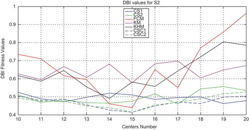
Figure 7. Variation of the XB index with respect to the number of clusters for the S2 data set with all methods.

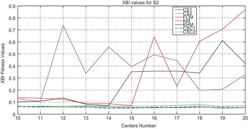
Figure 8. Variation of the WB index with respect to the number of clusters for the S2 data set with all methods.

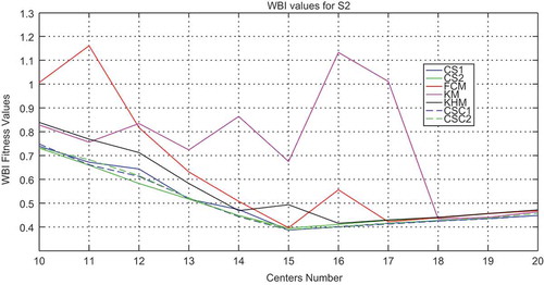
In the case of S2 data set, classical methods and CS algorithm have higher variance concerning DB and XB indices compared with CSC1 and CSC2 as can be observed in Figure 6 and Figure 7. For WB index, CS and CSC are stable; just classical methods present a high variance. Moreover, CSC1 and CSC2 have given the smallest values of all indices compared with the other algorithms.

In the case of the S2 data set, data are overlapped and OCN is also equal to 15.Table 3 shows the OCN obtained using the different indices by all the algorithms employed in this paper for the case of S2 data set.

Table 3. Comparison of the number of clusters obtained by the different algorithms in conjunction with the DB index, the XB index, and WB index – case of the S2 data set.

	DB		XB		WB
	K	Value	K	Value	K	Value
KM	15	0.5777	11	0.1061	18	0.4337
KHM	14	0.4903	14	0.0690	16	0.4148
FCM	15	0.4402	15	0.0702	15	0.3955
CS1	19	0.4623	19	0.0494	15	0.3876
CS2	17	0.4599	19	0.0643	15	0.3945
CSC1	15	0.4146	15	0.0474	15	0.3871
CSC2	15	0.4147	15	0.0498	15	0.3883

In Table 3 it is observed that all the indices give the right OCN for FCM method. With KHM method, the results are near to OCN (14 for XB and DB indices and 16 for WB index). The KM method finds the OCN with DB index and fails to obtain it with XB (11) and WB (18) indices. CS performs well with WB index and found 15 as OCN in all the experiments. CS fails to find the OCN with XB (19 for CS1 and CS2) and DB (19 for CS1and 17 for CS2) indices. Concerning CSC1 and CSC2, all the indices give the right number of OCN. Also, indices values are the smallest (marked in bold in Table 3) compared with those found with the other methods. We notice that by the use of overlapping data (case of S2), FCM, CSC1, and CSC2 obtain the OCN and, also in the case, the less value of indices is obtained with CSC1.

Real data results

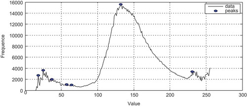
Remote-sensing data are very complex and overlapped in nature (Bandyopadhyay, Maulik, and Mukhopadhyay 2007); each pixel from the numeric image belongs to a landcover type considered as clusters. Some important classes are present in these images and can be identified easily. In the case of the first image (Figure 2(a)), we notice three sub clusters namely water, urban, bar soil, vegetation, fallows, and forest. Other method to have an idea about maximum clusters number consists to extract the number of peaks present in image histogram (Figure 9). Finally, the OCN of the first sub-scene used belongs to the interval. Regarding the second image (Figure 2(b)), we observe sea water, clouds, urban, water, forest, fallows, shadow, and bar soil. Knowing that the reflectance of the shadow is the same that the water in the used channels, we can consider that the subclusters sea water, water, and shadow are composing one class. According to these findings, we choose the interval. For the last image acquired by Alsat-2A (Figure 2(c)), we distinguish three kinds of fallows, urban, black rocks, and bar soil. Hence, the final number of clusters is included in the interval. The use of an interval by experts is explained by the difficulty of the study areas, particularly in the case of the last image due to its high spatial resolution.

Figure 9. The histogram of the first image data set.

Table 4, Table 5 and Table 6 summarize indices minimum values and their corresponding OCN obtained by all the methods for the case of Oran satellite image, Arzew satellite image and Tlemcen satellite image respectively. The lower values of indices are marked in bold for tables 4, 5 and 6.

Table 4. Comparison of the number of clusters obtained by the different algorithms in conjunction with the DB index, the XB index, and WB index – case of the first real image.

	DB		XB		WB
	K	Value	K	Value	K	Value
KM	3	0.4971	3	0.1164	6	0.9133
KHM	3	0.5792	3	0.1429	6	0.9931
FCM	3	0.5128	3	0.1167	6	0.9117
CS1	3	0.3562	5	0.0486	5	0,8441
CS2	3	0.3562	5	0.0465	5	0.8485
CSC1	3	0.3562	5	0.0486	6	0.8321
CSC2	3	0.3562	5	0.0459	6	0.8393

Table 5. Comparison of the number of clusters obtained by the different algorithms in conjunction with the DB index, the XB index, and WB index – case of the second real image.

	DB		XB		WB
	K	Value	K	Value	K	Value
KM	3	0.3922	3	0.0704	6	0.3536
KHM	3	0.4140	3	0.0810	5	0.3640
FCM	3	0.3874	3	0.0686	5	0.3504
CS1	3	0.3198	5	0.0377	5	0.3376
CS2	3	0.3199	5	0.0373	5	0.3375
CSC1	3	0.3198	4	0.0392	5	0.3342
CSC2	3	0.3198	6	0.0381	5	0.3336

Table 6. Comparison of the number of clusters obtained by the different algorithms in conjunction with the DB index, the XB index, and WB index – case of the third real image.

	DB		XB		WB
	K	Value	K	Value	K	Value
KM	3	0.3913	3	0.0980	8	0.2966
KHM	3	0.3976	3	0.1006	8	0.3039
FCM	3	0.3818	3	0.0937	8	0.2961
CS1	4	0.3489	7	0.0470	5	0.3406
CS2	3	0.3508	3	0.0485	5	0.3400
CSC1	4	0.3488	3	0.0484	8	0.2960
CSC2	4	0.3508	3	0.0488	8	0.2972

As shown in Table 4, all the methods as for the first image fail to obtain OCN with DB index and find K = 3 at DB minimum value. The smallest DB value is reached by CS1, CS2, CSC1, and CSC2. Concerning XB index, classical methods give K = 3 at XB minimum value and hence fail to have OCN. CS1, CS2, CSC1, and CSC2 results are close to OCN and give K = 5 with the smallest value of XB obtained by CSC2. For WB index, only CS1 and CS2 give K = 5 which is close to OCN. The other methods succeed to reach OCN with K = 6 and the smallest value of WB is given by CSC1.

From Table 5, it can be observed that OCN is not reached by all the methods using DB index and K = 3 for all the algorithms. CS1, CSC1, and CSC2 obtain the smallest DB value. OCN is reached by CS1, CS2, and CSC2 in the case of XB index. The other methods fail to have OCN and give K = 3 for classical methods and K = 4 for CSC1. Also, CS2 and CSC2 obtain the smallest XB values. Using WB index, all the methods find OCN with the smallest WB value obtained by CSC2.

As observed in Table 6, classical methods and CS2 fail to obtain OCN with DB index. However, CS1, CSC1, and CSC2 approximate OCN by giving K = 4 with the smallest DB value obtained by CSC1. For XB index, only CS1 give OCN with K = 7. Concerning WB index, CS1 and CS2 give OCN with K = 5. The other methods provide an approximate of OCN value with K = 8. It is noticed that in this case the WB smallest value is found by CSC1 although OCN is not reached by this method. This can be explained by the high spatial resolution of the image resulting in a big number of spectral classes present in the image. This number does not necessarily correspond to the number of thematic classes represented by OCN.

Figure 10 presents the classified images resulted from the clustering using different indices and all the methods concerning the first real image. Although there are numerical difference for different methods and validity indices, as it was shown in the previous paragraph, visually slight distinction is detected in classified images, especially for the second and the third images.

Figure 10. Clustered images of Oran with DB index (a i), XB index, (b i), and WB index (c i) using (i = 1) KM, (i = 2) KHM, (i = 3) FCM, (i = 4) CS1, (i = 5) CS2, (i = 6) CSC1, and (i = 7) CSC2.

Figure 10. Continued.

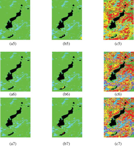
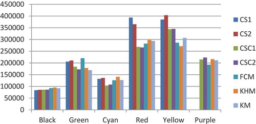
Concerning the first image, and as it can be observed in Figure 10, there is a minor visual variation between clustered images, notably for water region represented in black color for all the images case of the CSC2 algorithm. However, the histograms related to these images show that the different clusters have not the same number of pixels. As example we give the histogram concerning all the methods using WB index on the first image illustrated by Figure 11.

Figure 11. The number of pixels in each cluster obtained by all the methods using WB index.

From the experimental results, it can be concluded that among the three indices; WB index is the best in OCN choice for classical algorithms, and in using as fitness function for CS1, CS2, CSC1, and CSC2 algorithms. For the two other indices, DB index fails in all experiments to detect OCN with all the methods and detects fewer clusters than the other algorithms. Also, it can be observed that for XB index the number of clusters K is bigger than apparent clusters number calculated from clustered images. This can be explained by some clusters which contain few data and hence clusters will not be visible to naked eye. Figure 10 (b4, b5, b6, and b7) can be cited as examples.

Concerning the performance of the methods used in this paper, classical algorithms present more variance compared with CS and CSC algorithms which are more stable. Also, it can be observed that, in general, CSC1 and CSC2 perform better than CS1 and CS2. This can be explained by the fact that CSC operates as CS algorithm and exploits at the same time the best solutions of classical algorithms. Regarding the choice of the parameter α, CSC1 (α = 0.01) performed slightly better than CSC 2 (α = 0.1). This comes from the fact that a minor value of α allows a better exploration of neighbors of the solutions.

Finally, Figure 12(a), (b), and (c) shows the best results obtained for water body extraction, the application used in this work, by FCM from classical algorithms, and CSC1 and CSC2 from BIAs. In order to compare the different obtained water body extraction results, the ground truth is obtained by an expert in using supervised algorithm SVM and five regions of interest as illustrated in Figure 12(d). It is observed that the results of CSC2 are the most similar to ground truth.

Figure 12. Water body extraction results of the first image with WB index using (a) FCM, (b) CSC1, (c) CSC2, and (d) ground truth.

Conclusion

In this paper, a comparative study of classical clustering methods (KM, FCM, and KHM), CS algorithm, and Combined Cuckoo Search (CSC) method is carried out. Three validity indices are used each time in conjunction with CSC, namely DB index, XB index, and WB index. To evaluate the performance of all the employed methods and indices, synthetic and real data sets have been used.

In summary, CSC and CS are more stable compared with the other tested classical algorithms. Also, CSC in conjunction with WB index performs better than the other tested indices although they give in general the same OCN. In fact, the accuracy of clustering with WB index increases with BIAs (for example, the average accuracy increase with 0.1 for the first image with mean = 0.939 for classical methods and mean = 0.8357 for CSC). As an application of clustering problem, water body extraction is applied in this work; CSC2 performed better than the other algorithms concerning water identification.

Real images used in this paper have not showed big visual differences between classified images by the different algorithms despite the existence of numerical results diversity. The test of other remote-sensing images will be interesting for future works. Also, the use of multi-objective approach of CSC combining different indices is considered as a perspective of this research.

References

- Arbelaitz, O., I. Gurrutxaga, J. Muguerza, J. M. Pérez, and I. Perona. 2013. An extensive comparative study of cluster validity indices. Pattern Recognition 46 (1, January):243–56. doi:10.1016/j.patcog.2012.07.021.
- Azizah, B. M., M. Z. Azlan, and E. N. B. Nor. 2014. Cuckoo Search algorithm for optimization problems—a literature review and its applications. Applied Artificial Intelligence: An International Journal 28 (5):419–48.
- Bandyopadhyay, S., U. Maulik, and A. Mukhopadhyay. 2007. Multiobjective genetic clustering for pixel classification in remote sensing imagery. Geoscience and Remote Sensing 45 (5):1506–11.
- Bezdeck, J. C. 1984. FCM: Fuzzy C-Means algorithm. Computers and Geoscience 10:191–203.
- Bezdek, J. C. 1974. Cluster validity with fuzzy sets. Journal Cybernet 3:58–73.
- Bezdek, J. C. 1975. Mathematical models for systematics and taxonomy. in: Eighth International Conference on Numerical Taxonomy, San Francisco, CA. 143–65.
- Bong, C., and M. Rajeswari. 2011. Multi-objective nature-inspired clustering and classification techniques for image segmentation. Applied Soft Computing 11 (4):3271–82.
- Calinski, R. B., and J. Harabasz. 1974. Adendrite method for cluster analysis. Communicable Statist 3:1–27.
- Campbell, J. B. 2002. Introduction to Remote Sensing, Third ed. New York: CRC Press.
- Costa, J. A. F., and J. G. De Souza. 2011. Image segmentation through clustering based on natural computing techniques. In Inteck: Image segmentation, 57–82. Austria: InTech.
- Davies, D. L., and D. W. Bouldin. 1979. A cluster separation measure. IEEE Trans. Pattern Analysis and Machine Intelligence 1 (2):224–27.
- Dunn, J. C. 1973. A fuzzy relative of the isodata process and its use in detecting compact well separated clusters. Journal Cybernet 3:32–57.
- Gan, G., C. Ma, and J. Wu 2007. Data clustering: Theory, algorithms, and applications. ASA-SIAM Serieson Statistics and Applied Probability, SIAM, Philadelphia, ASA, Alexandria, VA.
- Gandomi, A. H., X.-S. Yang, and A. H. Alavi. 2013. Cuckoo search algorithm: A metaheuristic approach to solve structural optimization problems. Engineering with Computers 29 (1):17–35.
- Goel, S., A. Sharma, and P. Bedi. 2011. Cuckoo Search clustering algorithm: A novel strategy of biomimicry. World Congress on Information and Communication Technologies 916–21.
- Haibo, Y., W. Zongmin,Z. Hongling, and G. Yu. 2011. Water Body Extraction Methods Study Based on RS and GIS. Procedia Environmental Sciences 10:2619–2624.
- Halkidi, M., Y. Batistakis, and M. Vazirgiannis. 2002. Clustering validity checking methods: Part II. SIGMOD Record. Acm 31 (3):19–27.
- Khalid, N. E. A., N. M. Ariff, S. Yahya, and N. M. Noor 2011. A review of bio-inspired algorithms as image processing techniques. systems - second International Conference, ICSECS, In proceeding of. Software Engineering and Computer systems, 179: 660–73.
- Li, M., L. Xu, and M. Tang. 2011. An Extraction method for Water Body of Remote Sensing Image Based on Oscillatory Network. Journal of Multimedia 6 (3):252–260.
- MacQueen, J. 1967. Some methods for classification and analysis of multivariate observations. In Proc.5th berkeley symp mathematics, statistics and probability, 281–96. University of California Press, Berkeley, CA, USA.
- Manikandan, P., and S. Selvarajan. 2014. Data clustering using Cuckoo Search Algorithm (CSA). In Proceedings of the second international conference on soft computing for problem solving (SocProS 2012), ed B. V. Babu, A. Nagar, K. Deep, M. Pant, J. C. Bansal, K. Ray, and U. Gupta, Vol. 236, 1275–83. Heidelberg: AISC, Springer.
- Maulik, U., and S. Bandyopadhyay. 2003. Fuzzy partitioning using a realcoded variable-length genetic algorithm for pixel classification. IEEE Transactions Geoscience and Remote Sensing 41 (5):1075–81.
- Ming-Der, Y. 2007. A genetic algorithm (GA) based automated classifier for remote sensing imagery. Journal Canadien De Télédétection 33 (3):203–13.
- Pakhira, M. K., S. Bandyopadhyay, and U. Maulik. 2005. A study of some fuzzy cluster validity indices, genetic clustering and application to pixel classification. Fuzzy Sets and Systems 155:191–214.
- Payne, R. B., M. D. Sorenson, and K. Klitz. 2005. The Cuckoos. New York: Oxford University Press.
- Reynolds, A., and M. A. Frye. 2007. Free-flight odor tracking in Drosophila is consistent with a mathematically optimal intermittent scale-free search. PLoS ONE 2 (4):354.
- Saida, I. B., K. Nadjet, and B. Omar. 2014. A new algorithm for data clustering based on Cuckoo Search optimization. Genetic and Evolutionary Computing 238:55–64.
- Senthilnath, J., V. Das, S. N. Omkar, and V. Mani. 2013. Clustering using lévy flight Cuckoo Search. In Proceedings of seventh international conference on bio-inspired computing: Theories and Applications,(BIC-TA 2012), ed J. C. Bansal, P. Singh, K. Deep, M. Pant, and A. Nagar, Vol. 202, 65–75. Heidelberg: AISC, Springer.
- Swagatam, D., and K. Amit. 2009. Automatic image pixel clustering with an improved differential evolution. Applied Soft Computing 9 (1):226–36.
- Thangavel, K., and K. Karthikeyani Visalakshi. 2009. Ensemble based distributed K- harmonic means clustering. International Journal of Recent Trends in Engineering 2 (1):125–29.
- Tong, H., Z. Man, and L. Xiang. 2009. Applications of computational intelligence in remote sensing image analysis. In Computational intelligence and intelligent systems, communications in computer and information science, Vol. 51, 171. ISBN. 978-3-642-04961-3. Berlin Heidelberg: Springer-Verlag.
- Tuba, M., M. Subotic, and N. Stanarevic. 2012. Performance of a modified Cuckoo Search algorithm for unconstrained optimization problems. WSEAS TRANSACTIONS on SYSTEMS 11 (2):62–74.
- Valian, E., S. Mohanna, and S. Tavakoli. 2011. Improved cuckoo search algorithm for feedforward neural network training. International Journal Artificial Intelligent Applications 2 (3):36–43.
- Walton, S., O. Hassan, K. Morgan, and M. R. Brown. 2011. Modified cuckoo search: A new gradient free optimization algorithm. Chaos Solitons Fractals 44 (9):710–18.
- Xie, X. L., and G. Beni. 1991. A validity measure for fuzzy clustering. IEEE Transactions on Pattern Analysis and Machine Intelligence 13 (8):841–47.
- Yang, X.-S. 2010. Nature-inspired Metaheuristic Algorithms. Second Edition, United Kingdom: Luniver Press.
- Yang, X.-S., and S. Deb. 2009. Cuckoo search via Lévy flights. World Congress on Nature & Biologically Inspired Computing 210–14.
- Yang, X.-S., and S. Deb. 2014. Cuckoo search: Recent advances and applications. Neural Comput and Application 24 (1):69–174.
- Zexuan, J., X. Yong, C. Qiang, S. Quansen, X. Deshen, and D. F. David. 2012. Fuzzy c-means clustering with weighted image patch for image segmentation. Applied Soft Computing 12:1659–67.
- Zhang, B. 2000. Generalized K-harmonic means boosting in unsupervised learning. Technical Reports, Hewllet Laborotories, Palo Alto.
- Zhang, L., L. Mao, H. Gong, and H. Yang 2013. A K-harmonic means clustering algorithm based on enhanced differential evolution. 2014 Sixth International Conference on Measuring Technology and Mechatronics Automation: 13–16.
- Zhao, Q. 2012. Cluster validity in clustering methods. Ph.D. dissertation, University of Eastern Finland.
- Zhao, Q., and P. Fränti. 2014. WB-index: A sum-of-squares based index for cluster validity. Knowledge and Data Engineering 92:77–89.
- Zhao., J., X. Lei., Z. Wu., and Y. Tan. 2014. Clustering using improved cuckoo search algorithm. The Fifth International Conferencce on Swarm Intelligence (ICSI 2014), Hefei, China, October 17-20. Springer, LNCS 8794: 479–88.