A Modular Real-time Tidal Prediction Model based on Grey-GMDH Neural Network

ABSTRACT

Real-time prediction of tidal level is of great significance for activities of human beings in the fields of marine and coastal engineering. However, the disturbance factors of tidal level are very intricate, which deteriorate the tidal prediction accuracy. To improve the accuracy of real-time tidal-level prediction, a modular real-time tidal-level prediction approach is proposed based on the grey group method of data handling (Grey-GMDH) neural network. The modular model is composed of astronomical tide parts caused by celestial bodies’ movement and the nonastronomical tide parts caused by various meteorological and other environmental factors. The GMDH is a polynomial network that is commonly used in prediction and pattern recognition. However, GMDH is sensitive to nondeterministic time series, which would result in low accuracy of prediction. In this study, the grey prediction theory is introduced into the GMDH prediction model to alleviate the unfavorable effects of uncertainty caused by various environmental factors and the adverse effects caused thereby on the prediction accuracy. In this study of tidal prediction, the Grey-GMDH model is used to predict the nonastronomical tide parts, whereas the conventional harmonic analysis model is used to predict the astronomical tide parts. The final prediction result is achieved by combining the estimation outputs of the harmonious analysis model and the Grey-GMDH model. Measured tidal-level data of San Diego tidal station is selected as the testing database. Simulation and experimental results confirm that the proposed approach can achieve real-time predictions for tidal level with high accuracy, satisfactory convergence and stability.

Introduction

Tidal-level prediction is an indispensable activity for the design of coastal constructions such as wharves and harbors. Real-time tidal prediction also has a great influence on the decision-making procedures of vessels or drilling platforms in offshore areas. Accurate real-time tidal prediction is particularly crucial in operation scheduling, such as making navigating plan of ships through shallow water or bridge. Under these conditions, decision, taking into account the under-keel clearance or the water depth under bridge, can be adopted based on the hourly tidal-level forecast. Furthermore, tidal information is a significant influential factor for navigation scheduling of a platform’s operation planning. Consequently, the accurate real-time forecasting of tidal level in the fields of coastal and ocean engineering is an issue of concern.

In recent years, the most popular technique in tidal research is the harmonic analysis method, in which the components of tides can be expressed as the superposition of several sinusoidal constituents determined by the harmonic analysis method. In addition, the harmonic analysis method remains the basis for long-term tidal-level prediction (Lee 2006; Lee and Jeng 2002). Nevertheless, there are some drawbacks in practical applications of the harmonic analysis method. First of all, the necessary components of harmonic analysis need to be determined by a considerably long period of tidal-level records. However, long-term tidal-level records may not be obtained owing to the high cost of the in situ monitoring data. Second, the only consideration of this prediction model is the effects of celestial bodies and coastal topography like the framework of the coastline and the profile of the seabed. Consequently, it cannot express the complicated time-varying meteorological impacts on tide, which are produced by meteorological elements like sea wind, atmospheric temperature and pressure, sea ice, sea rainfall, etc. In addition, there are some other time-varying factors such as river discharge and fluctuation, which will also have an impact on tidal level at the estuary region. Consequently, the prediction accuracy of the harmonic analysis model is quite low under some circumstances.

Nowadays, with the rapid development of artificial intelligence technology such as neural network and fuzzy logic, the artificial intelligence technology has been widely used in the fields of engineering computation and simulation (Yin and Wang 2013; Yin et al. 2014) due to its strong nonlinear mapping and self-learning ability. Artificial neural networks (ANNs) have proved to be of versatile utility in engineering optimization and computation fields (Haykin 1999), owing to their excellent abilities of nonlinear mapping, generalization and self-learning. The neural network based on error back propagation (BP) is the most popular and practical neural network, and it is widely used in tide forecasting (Lee 2004, 2008). Variable-structure radial basis function neural network constructed by sequential learning is proposed for tidal prediction (Yin, Zou, and Xu 2013). One-day-ahead tide prediction of the west coast of India New Mangalore tide station was carried out using neural networks (Jain and Deo 2007); the estimation of monthly mean significant wave heights using ANN and regression methods (Günaydın 2008) and the development of a regional neural network were proposed for coastal water-level predictions (Huang et al. 2003).

The group method of data handling (GMDH) neural network (Farlow 1981, 1984) is also referred to as polynomial neural network. GMDH network is a kind of learning model based on heuristic self-organizing theory, which was proposed by AG Ivakhnenko in 1967. It is a kind of local feedforward network commonly used in prediction (Kordnaeij et al. 2015; Najafzadeh, Barani, and Azamathulla 2014, 2013). Unlike the fixed structure of traditional error BP neural network, the GMDH network structure is variable, which is constantly changing in the process of simulation training. The structure of the GMDH prediction model is determined according to the input and output information. The relationship between the dependent variable and the independent variable is obtained based on the regression method. The main mechanism of GMDH is to build an analytical function in a feedforward network based on a quadratic node transfer function, whose coefficients are obtained using the regression method combined with emulation of the self-organizing approach (Farlow 1984). Actually, the model parameters of the GMDH network are estimated utilizing the least square algorithm. Hwang (2006) used a fuzzy GMDH-type neural network model for the prediction of mobile communication, and it was proved that the proposed method was suitable for the prediction of complex systems. Srinivasan (2008) used the GMDH network for energy demand prediction, and it was significantly more precise and less labor-intensive than conventional time-series and regression-based models. The GMDH model is the optimal simplified model that possesses higher accuracy and simpler structure than conventional neural network models (Ketabchi et al. 2010). However, the conventional GMDH network is sensitive to the nondeterministic time series, which deteriorate its prediction accuracy.

To overcome these drawbacks and facilitate its practical applications, a modular Grey-GMDH prediction model is proposed to improve the performance of the conventional GMDH network. Modularization is the process of dividing the system into several modules with different attributes when analyzing and solving a specific problem (Knoernschild 2012). The tidal component is divided into astronomical tide parts and nonastronomical tide parts. The harmonic analysis method (Vladimir 2004) is used to predict the astronomical tidal parts, whereas the Grey-GMDH forecasting method is used to predict the nonastronomical tidal parts with strong nonlinearity. The proposed method combines the advantages of the two methods: the harmonic analysis model can achieve long-term, stable astronomical tide forecast and the Grey-GMDH model can complete the nonlinear fitting and prediction of tides with high accuracy. In this study, the grey predicting model is introduced in the GMDH tidal prediction model, which will weaken the impacts of various uncertain environmental factors. In addition, the correlation analysis is utilized to analyze the time series of the tidal-level data for determining the input dimensions of the Grey-GMDH prediction model; the final prediction result is achieved by combining the estimation outputs of the harmonious analysis model and the Grey-GMDH model. The observed tidal-level data of San Diego tidal station is selected as the testing database. The results of the simulation have confirmed that the proposed novel method can provide predictions for real-time tidal level with high accuracy, excellent convergence and satisfactory stability.

The rest of the paper is organized as follows. A brief description about harmonic analysis is given in section 2; the basic principle and structure of the Grey-GMDH model is represented in section 3; the modular prediction model is provided in section 4; simulation results and detailed discussions are displayed in section 5; and conclusions are provided in the last section.

Harmonic analysis

Theoretically explaining, tides are periodic vertical movements of the sea level. The origin of tide is the tide-generating force of celestial bodies in space, which is a combination of the centrifugal and gravitational forces between the earth and the celestial bodies.

The most commonly and widely utilized approach is the harmonic analysis method in practice. The harmonic analysis approach decomposes the complicated tides into a couple of periodic constituents, each of which is generated by a hypothetical celestial body. At moment t, for a definite tide station with the height of tide h(t), it can be expressed as

(1)

where H₀ is the mean sea level, f_k is the node factor, σ_k is the angular velocity of tidal components, (v₀ + u)_k is the initial phase of the tidal components, H_k is the amplitude of tidal components, g_k is the time interval from the moments the celestial body passes the upper transit meridian to the moments when high water occurs and H_k and g_k are the harmonic analysis constants.

In practical theory, the quantity of tidal components may be quite huge; fortunately, most of the tidal components can be ignored because of their smaller amplitude (H_k) and longer period (g_k). In actual calculation, Eq. (1) can be rewritten as

(2)

where H₀ is the mean sea level, n is the number of components, h_k is the amplitudes of tidal components, ω_k is the angular velocity of tidal components and ϕ_k is the initial phase of the tidal components.

The harmonic analysis method is widely used in tide prediction because of its stable prediction performance and simple calculation process. Although the harmonic analysis method is extensively used for tidal-level prediction, the drawback of the conventional harmonic analysis method is quite apparent: the harmonic constant of this approach requires a large number of measured tidal data, which is a laborious and time-consuming process.

GMDH model

GMDH neural network

GMDH is a technology based on evolutionary computation, and it is based on the dimension of the input variables, the structure of the network model and the network parameters to carry out a series of evolution, heredity, and variation and selection operations (Ivakhnenko 1971, Ivakhnenko and Ivakhnenko 2000). The typical training GMDH model is shown in Figure 1.

Figure 1. Structure of the GMDH neural network.

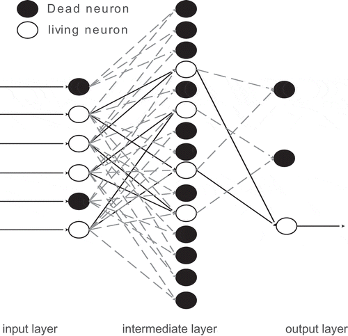
When establishing the GMDH network model, the sample data is divided into two parts: training data set and checking data set. For the establishment of the predictive control model, the sample data is divided into training sets, checking sets and predicting sets. One of the remarkable features of the GMDH model is the utilization of external information. The training data set is used for modeling (parameter estimation and structure synthesis), whereas the information of the checking data set is used only when selecting the optimal complexity model. The basic theory of the GMDH model is that the sample data that influences the system are used to generate a number of candidate models, and an optimal complexity model is selected from the candidate model sets based on the external criterion. The multilayer algorithm of the GMDH algorithm is introduced in this study, and the main implementation step of the multilayer algorithm includes two important links: the utilization of internal criteria for establishing a competitive model (intermediate candidate model) and the utilization of the external criteria (selection criterion) for selecting the optimal complexity model. The external criterion of the GMDH algorithm is a quite significant section; taking into account the particularity of the prediction and control (Mozaffari et al. 2016; Najafzadeh, Barani, and Hessami-Kermani 2015) of the tidal level, the root mean square error (RMSE) is chosen as the standard of the external criterion.

According to the theory of GMDH network, a GMDH model is represented as a large number of neurons in which different pairs of neurons in each layer are joined by a quadratic polynomial and thus generates new neurons in the new layer. For the sake of generating output value y^’ for a certain input vector X = (x₁, x₂, x_{3 …} x_n) as close as possible to its real output value y, the basic definition of the identification problem of the model is to figure out a function f^’’ that can be substituted for the realistic function f approximately. Consequently, for a given set of measured data in a multi-input and single-output model:

(3)

The GMDH network can be trained to predict output value y^’ for any certain input vector X = (x_j1, x_j2, x_j3… x_jn), that is,

(4)

The simulation purpose of the whole network model is to ensure that the predictive value y^’ can be more close to the measured value y; the square of the differences between the measured data and the predicted data is utilized to determine the GMDH neural network, that is,

(5)

Generally, the relationship between the input and output variables of the GMDH network can be represented by a complex discrete form of the Volterra functional series (Ivakhnenko 1971):

(6)

where (6) is the Kolmogorov–Gabor polynomial (Ivakhnenko 1971). X = (x₁, x₂, x₃ … x_M) represents the input vector, y represents the output variable and the number of input variable m is set to 4, which is based on the correlation analysis of the tidal-level data in this study. The transfer functions of the network, which connects neurons in different layers, can be represented in the form of

(7)

The coefficients a_i, which are initialized to random number at the beginning of the program in (7), are calculated by the least squares regression means (Amanifard et al. 2008). In the fundamental formation of the GMDH algorithm, the linear regression polynomial that optimal fits the measurements (y_i) in the form of (6) is established by utilizing all the possibilities of two input variables in the total of n input variables. Several optimal neurons that meet the chosen criterion (external criterion) between the outputs of the first layer are selected as the input into the second layer with all combinations of different pairs of them. The new generation (layer) of the network is obtained by the combination of the lower-order polynomials at each generation (layer) by employing the GMDH algorithm. The basic steps of the self-organizing algorithm are briefly summarized as follows: establishing the input and associated output sample data for the GMDH prediction model and dividing them into learning and checking data sets, determining the dimension of input data and computing coefficients of the regression polynomial for each pair of input variables (x_i, x_j) together with the corresponding output variables in the learning data sets by using the least square method. Calculating the m(m − 1)/2 high-order variables of the initial input vector X = (x₁, x₂, x₃ … x_M) to evaluate the output y, m is the dimension of the input variables. The learning algorithm produced a large number of new variables (neurons): , , …, (m_l = m_l−1(m_l−1 − 1)/2) in the previous generation (layer), where m_l denotes the dimension of input variables for the l generation (layer). Each of these new generated variables is evaluated by judging which variable is the optimal estimation of the dependent variable. The columns of the new generated variable are sorted. A random critical value R is determined by model analysis. Each column of with RMSE_j > R is eliminated, where j is the number of the network layer. The remaining variables are selected as the input variables for the next new generation (layer). This procedure is repeated until the introduction of new neurons cannot induce an obvious enhancement in the approximation capabilities of the model or the stop criterion is set in advance (Chao, Ferreira, and Liu 1988; Widrow and Lehr 1990).

Grey-GMDH neural network

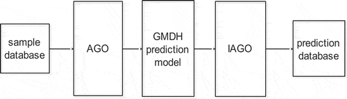
The theory of the grey system was proposed by professor Deng (Deng 1986). The grey system model is based on the principle of “Grey Box” with small samples and incomplete information, which implies that the available information is not sufficient. The grey model can reveal the inherent regularity of a raw data sequence by using the data-mining and analysis methods. Practical results have proved the effectiveness of the Grey prediction model (GPM) in processing poor information with limited amount of data (Ma and Liu 2015; Tien 2009). Generally speaking, GPM consists of three essential processes: (1) accumulated generation operation (AGO) by accumulating the raw time-series data; (2) grey prediction based on the accumulated newfound time-series data in GPM, where the GPM is replaced by the GMDH model in this study, respectively; and (3) inverse accumulated generation operation (IAGO), where the time series in GPM, which is substituted for the Grey-GMDH model, is converted back to its original form to realize the predicted result. The GPM (1, 1), with a single variable, is normally the most commonly used forecasting model. The brief description of the prototype of GPM (1, 1) is as follows:

(7)

where x⁽⁰⁾(i) represents the time-series database in primary time series x⁽⁰⁾ at time step of i, and the bracketed number in the superscript stands for the order of the GPM.

A newfound time series x⁽¹⁾ is generated by the AGO process:

(8)

where x⁽¹⁾(k) =⁽⁰⁾(i).

By means of the AGO procedure, the preceding asymmetric and disordered database could become exponentially preformed so that the system performance can be characterized by the implementation of the differential equation. The time-response solution for forecast is subsequently completed by solving the differential equation:

(9)

(10)

Eq. (10) is the solution of Eq. (9).

Finally, the prediction result is achieved by the IAGO process:

(11)

where a and b are completed by means of the linear least squares (LLS) method. ⁽¹⁾(k + 1) and ⁽¹⁾(k) are the prediction results of ⁽¹⁾(k + 1) and ⁽¹⁾(k); and ⁽⁰⁾(k + 1) is the prediction result of ⁽⁰⁾(k + 1).

The schematic of the GMDH model based on the grey prediction system is shown in Figure 2.

Figure 2. Schematic of Grey-GMDH prediction systems.

Modular tide prediction model

Depending on the origin of the tide, tidal-level prediction can be divided into two parts: astronomical tide parts caused by celestial bodies’ movement and nonastronomical tide parts caused by various meteorological factors such as sea wind and sea wave. Astronomical tide, which is mainly caused by the tidal force of celestial bodies, has a notable time-varying characteristic, whereas nonastronomical tide shows strong nonlinearity. In this study, the conventional harmonic analysis method is implemented to predict the astronomical tide section, and the residual tide section is predicted by the Grey-GMDH prediction model. The residual section is a complicated association caused by the topography as well as hydrological and meteorological factors such as sea wind, sea wave and seawater temperature. The Grey-GMDH prediction model could fit the residual tide section, which shows obvious nonlinear performances accurately. The final prediction model is composed of the harmonic prediction model and the Grey-GMDH prediction model. The composition and the training process of the final modular prediction model are shown in Figure 3.

Figure 3. Flow chart of the modular tidal prediction model.

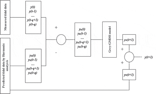
In the modular prediction model, the observed tidal data y(t), y(t–1),… y(t–q) is set as the input of the model. Here y_H, y_H(t–1), …, y_H(t–q) is the tidal prediction value obtained by the harmonic prediction method and y_R, y_R(t-1), …, y_R(t-q) is the difference between y and y_H. Finally, the ultimate modular prediction model is the combination of the harmonic prediction model and the Grey-GMDH prediction model. Eventually, the predictive tidal level y(t + 1) is the association of y_H(t + 1) and y_R(t + 1).

Simulation of the tidal-level prediction

Tidal data analysis

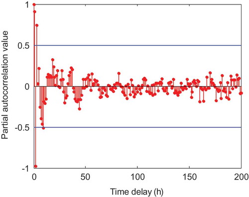
The concept of correlation analysis (Young and Shellswell 1972) originates from signal processing and analysis; correlation analysis reflects how the correlation between any two values in a time series is changed over time. In addition, autocorrelation analysis depicts the correlation between neighboring variables of the time series. Autocorrelation function and partial autocorrelation function are an effective way of analyzing and dealing with complex time series (Nezli and Li 2003; Zhao et al. 2014): the autocorrelation function describes the relationship between the adjacent variables of time series, whereas the partial correlation function eliminates the influence of other intermediate variables in time series. In tidal data analysis, the time series of the tidal level is affected by many variable factors that are difficult to be measured by nautical equipment, thereby making it difficult to calculate the contribution to tidal level. Consequently, the correlation analysis method is utilized to analyze the correlation between the time series of tidal level and then to determine the input dimension of the Grey-GMDH prediction model. In this study, a correlation value of 0.5 is selected as a reference standard to determine the input dimension, and the analysis results are shown in Figures 4 and 5. Figure 4 shows that the autocorrelation coefficient of the tidal-level time-series data is tailing. Meanwhile, the autocorrelation coefficient reaches gradually closer to zero and tends to be stable. Furthermore, Figure 5 shows that the partial autocorrelation coefficient is four-order truncation. To summarize, the correlation analysis demonstrates that the time-series value from t-1 to t-4 moment has a significant relevance with the time-series value of moment t, which can be selected as the input of the modular prediction model.

Figure 4. Autocorrelation analysis of tidal data.

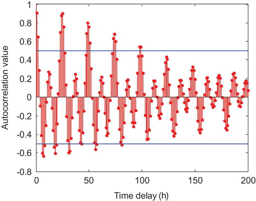
Figure 5. Partial autocorrelation analysis of tidal data.

Experimental measurements of San Diego tidal station over the duration from 1 January 00:00 GMT, 2015, to 7 September 23:00 GMT, 2015, with a time resolution of 1 h, with a total of 6000 pairs of observed tidal-level data, are chosen as the testing and training database. The modular model accomplishes initialization training stage by employing the advanced 4200 samples of measured tidal data, which includes 70% of the training data and 30% of the checking data, and the residual sections are supplied to the modular prediction model for a one-step-ahead prediction. The linear least square algorithm is chosen as the internal criterion of the prediction model, which is the generation principle of the intermediate candidate model. Moreover, the RMSE is chosen as the standard of the external criterion. All the measured tidal-level data applied in this study can be obtained from the website http://co-ops.nos.noaa.gov/.

In this study, the structure of the prediction model, which includes one input layer of four-input-nodes, four hidden layers and one output layer of one-output-nodes, is set to total six layers; the maximum number of neurons in each intermediate layer is limited to 25 in order to prevent the GMDH from tending to produce an exceedingly complicated network when it comes to highly nonlinear models owning to its limited general structure (quadratic two-variable polynomial) (Park et al. 2004).

For a further comprehensive comparison of the simulation result, the RMSE, the mean square error (MSE), the mean absolute error (MAE), the standard deviation (SD) and the mean error (ME) are introduced as an evaluation indicator to evaluate the performance of the proposed prediction model. The concepts of RMSE, MSE, MAE, SD and ME are described in Eqs. (12)–(16):

(12)

(13)

(14)

(15)

(16)

where n is the number of sample data, μ represents the arithmetic mean value of the observed data, y_k represents the value of the observation and _k denotes the value of prediction.

Tidal-level prediction using the harmonic analysis model

The tidal-level prediction of San Diego tidal station using the harmonic analysis prediction method is illustrated in Figure 7 together with the observed ones, which are exhibited on the website of NOAA, with a time resolution of 1 hour.

Figure 6. Location map of the tidal-level station on the California coast of the United States.

(Source: http://co-ops.nos.noaa.gov/)

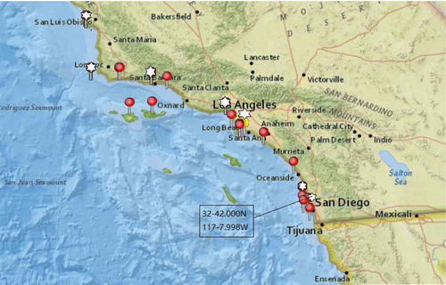
Figure 7. Simulation results using the harmonic analysis method.

(one-step-ahead prediction of San Diego tidal station)

It can be clearly seen from Figure 7 that the predicted value of the tidal level falls below the observation value from the beginning to the end, which explains that the tidal level could be affected by unexpected factors of environmental changes, such as the rough sea or heavy sea-surface wind. In addition, there exists a comparatively large sustained deviation with the correlation coefficient (CC) of 0.9973, which is illustrated in Figure 8. The sustained offset between the predicted and observed tidal levels reaches up to 1 foot, and the prediction error of the harmonic analysis model is in the range of [–0.1,1], which can be seen from the error diagram in Figure 7. In addition, the distribution center of the prediction error of the prediction model is centered on about 0.4 feet, instead of tending to zero, and the harmonic prediction model also has a larger prediction error, which can be seen from the error histogram analysis in Figure 7.

Figure 8. Scatter diagram of the measured and predicted results using the harmonic method.

Figure 8 is the scatter diagram of the measured and predicted results by using the harmonic analysis method. The red line in Figure 8 denotes the measured value of the tidal level and the green mark in Figure 8 represents the predicted value of the tidal level using the harmonic analysis method.

Tidal-level prediction using the GMDH model

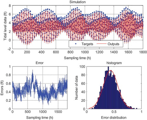
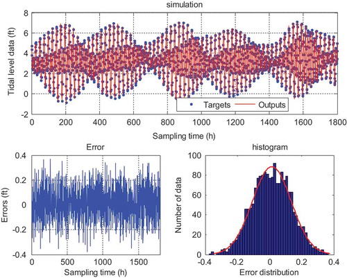
Figure 9 is the simulation diagram of the GMDH model. It can be analyzed from Figure 9 that the fitting consistency between the GMDH prediction value and the measured value is obviously better than the harmonic analysis model; the prediction error of the GMDH model is in the range of [–0.4,0.4], which can be seen from the error diagram in Figure 9. Furthermore, the distribution center of the prediction error of the GMDH model is basically concentrated in about 0. Nevertheless, the error distribution of the GMDH model is not uniform, and the error fluctuation range is relatively larger, which can be seen from the error histogram analysis in Figure 9.

Figure 9. Simulation results using the GMDH model.

(one-step-ahead prediction of San Diego tidal station)

Tidal-level prediction using the modular GMDH model

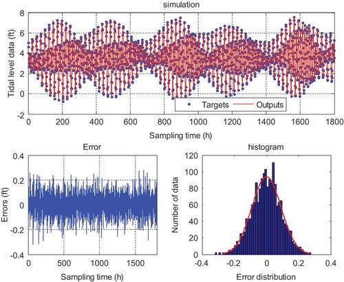
It can be apparently recognized from Figure 10 that the prediction values produced by the modular GMDH prediction method coincide well with the observed tidal data than the harmonic method or the GMDH method. The modular prediction model consists of two sections: the harmonic analysis prediction model, which takes into consideration the celestial bodies’ movement, and the GMDH prediction model, which considers the residual sections. Consequently, the prediction results of the tidal level are more accurate than merely utilizing the harmonic analysis method or the GMDH method. Furthermore, the prediction error of the modular GMDH prediction model is in the range of [–0.3, 0.3], which can be seen from the error diagram in Figure 10. It illustrates that the prediction accuracy is significantly improved compared with the direct prediction model of GMDH and the harmonic prediction model. Moreover, the distribution of the error of the modular model gradually tends to be uniform and smooth, the error distribution center is almost 0 and the error distribution is symmetrical with respect to the distribution center.

Figure 10. Simulation results using the modular GMDH model.

(one-step-ahead prediction of San Diego tidal station)

Tidal-level prediction using the Modular Grey-GMDH model

The 1-h-head tidal-level forecasting results using the Modular Grey-GMDH method are represented in Figure 11, together with the real observations. It can be noticed from the error diagram in Figure 11 that there is no large continuous offset between the forecasted values and the measured ones. In addition, the forecasted results locate around the actual ones conformably, which can also be obtained from Figure 12. The closeness between the observed tidal values and the forecasted ones can be further validated by the corresponding higher CC of 0.9993, as indicated in Figure 12. In addition, the prediction error of the Modular Grey-GMDH model is in the range of [–0.2, 0.2], which can be seen from the error diagram in Figure 11. Moreover, the error distribution center almost completely tends to 0, the error distribution is more uniform, the center is almost completely symmetrical with respect to the error distribution center and the error fluctuation range is significantly reduced compared to the previous three models, which is illustrated from the error histogram analysis in Figure 11. In conclusion, this proposed model significantly improves the prediction accuracy of tidal level.

Figure 11. Simulation results using the modular Grey-GMDH model.

(one-step-ahead prediction of San Diego tidal station)

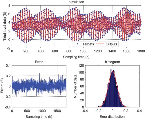
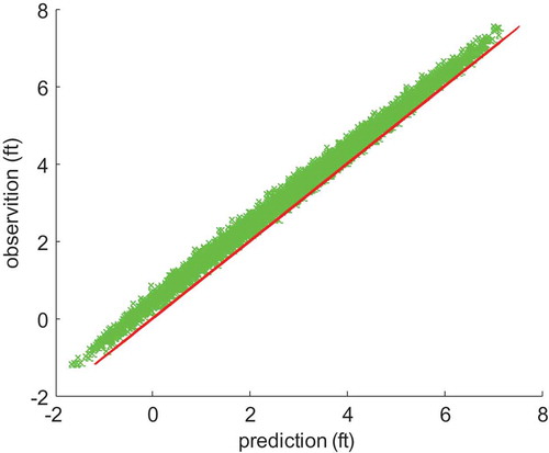
Figure 12. Scatter diagram of the measured and predicted results by the modular Grey-GMDH model.

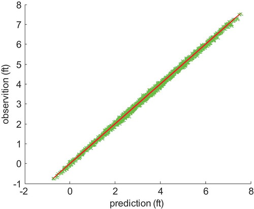
Figure 12 is the scatter diagram of the measured and predicted results by using the modular Grey-GMDH method, in which the red line denotes the measured value of tidal level and the green mark represents the predicted value of tidal level by using the modular Grey-GMDH method.

To further quantitatively validate the predictive performance of the modular Grey-GMDH prediction model proposed in this study, comparative simulations are conducted by using methods of harmonic analysis, GMDH and modular GMDH. Detailed simulation results based on the same simulation environment, the same simulation parameters and the same measured tidal data of San Diego tidal station are shown in Table 1.

Table 1. Tidal-level simulation results of San Diego tidal station.

Model	RMSE(ft)	MSE(ft)	Mean error(ft)	Standard deviation(ft)
Harmonic analysis	0.4583	0.2100	0.4388	0.1322
GMDH	0.1216	0.0147	0.0143	0.1208
Modular GMDH	0.0906	0.0082	0.0006	0.0908
Modular Grey-GMDH	0.0638	0.0040	0.0050	0.0636

It is clearly seen from Table 1 that the corresponding error value of the modular Grey-GMDH prediction model is the smallest one of the four prediction models. As a consequence, the experimental results demonstrate that the proposed modular GMDH model has a higher forecasting accuracy for tidal-level prediction.

Different time spans of time-series prediction will affect the magnitude of prediction error. To further compare the accuracy of the conventional GMDH model and the modular Grey-GMDH model in the prediction of tidal level, simulation experiments of different time spans are carried out based on the same observed tidal-level data. Simulation results are represented in Tables 2 and 3.

Table 2. Tidal prediction results for San Diego using the conventional GMDH model.

Prediction time span	RMSE (ft)	MAE (ft)	MSE (ft)	Mean error (ft)	Standard deviation(ft)	CC	Steps	Times (s)
1-h-ahead	0.2793	0.2195	0.0780	0.0543	0.2741	0.9868	1800	1.6443
2-h-ahead	0.4508	0.3570	0.2033	0.1432	0.4276	0.9678	1800	2.0528
3-h-ahead	0.7199	0.5626	0.5182	0.3428	0.6332	0.9292	1800	1.9866
6-h-ahead	1.0116	0.8145	1.0233	0.5754	0.8323	0.8720	1800	1.9870
12-h-ahead	1.0370	0.8357	1.0753	0.5798	0.8600	0.8617	1800	1.9778
24-h-ahead	0.3175	0.2504	0.1008	0.0173	0.3171	0.9822	1800	2.2911
48-h-ahead	0.5917	0.4723	0.3501	0.0493	0.5898	0.9377	1800	2.0225

Table 3. Tidal prediction results for San Diego using the modular prediction model.

Prediction time span	RMSE (ft)	MAE (ft)	MSE (ft)	Mean error (ft)	Standard deviation(ft)	CC	Steps	Times (s)
1-h-ahead	0.0926	0.0086	0.0085	0.0121	0.0918	0.9985	1800	1.6859
2-h-ahead	0.1019	0.0812	0.0104	0.0161	0.1006	0.9984	1800	2.1701
3-h-ahead	0.1076	0.0862	0.0116	0.0197	0.1058	0.9984	1800	2.0221
6-h-ahead	0.1134	0.0906	0.0129	0.0228	0.1111	0.9985	1800	2.0910
12-h-ahead	0.1053	0.0838	0.0111	0.0247	0.1024	0.9982	1800	2.0963
24-h-ahead	0.0912	0.0716	0.0083	0.0211	0.0887	0.9986	1800	2.0955
48-h-ahead	0.1209	0.0930	0.0146	0.0356	0.1156	0.9977	1800	2.0187

It can be noticed from Table 2 that the RMSEs of tidal-level prediction using the conventional GMDH method are 0.2793 and 0.4508 for 1-hour-ahead and 2-hours-ahead forecasting, respectively. In addition, the values of RMSE are in the range of 0.2793 and 1.0370 for 3 or more hours-ahead predictions. Furthermore, the RMSE values of tidal-level prediction by using the modular Grey-GMDH method for 1-hour-ahead and 2-hours-ahead predictions are 0.0926 and 0.1019, respectively, which can be obtained from Table 3, and the values of RMSE are in the range of 0.0926 and 0.1209 for 3 or more hours-ahead forecasting, which illustrates that the proposed novel modular prediction method is able to provide stable and reliable prediction results for tidal-level forecast with satisfactory prediction accuracy. In addition, with the increase of the forecasting time interval, the proposed novel method also exhibits higher forecasting accuracy compared with the conventional GMDH method, which can also be obtained from the corresponding error value illustrated in Table 2 and Table 3. Moreover, the time consumption of the whole simulation process has no obvious increase, which validates the high efficiency of the proposed approach.

Performance of tidal-level prediction

To validate the prediction accuracy, universality and generalization ability for longer time scope tidal-level prediction, simulation experiments were carried out based on the observed tidal-level data of six different tidal stations located on the west coast of California in America. Simulation results of multistep tidal prediction based on the same simulation environment and the same simulation parameters are shown in Table 4. The time duration of the observed tidal-level data of the six tidal stations is the same as that of the San Diego tidal station. It is revealed in Table 4 that the proposed approach can achieve stable and accurate tidal predictions for the observed tidal data of the six different tidal stations, which are shown in Figure 6. Furthermore, the simulation results also illustrate that the proposed modular prediction method is able to provide stable and reliable prediction results for tidal-level forecast with satisfactory prediction accuracy. It is also noticed that the number of network layers of the GMDH optimal complex model is set in advance and the same network parameters are used for tidal prediction of different tidal stations in this study. As a consequence, an optimal method for self-selection of the network layers and further adjustment of the network parameters should enhance the performance of the proposed approach.

Table 4. Tidal prediction results using the modular prediction model based on the Grey-GMDH model.

Tidal station	Prediction span(h)	RMSE (ft)	MAE (ft)	MSE (ft)	Mean error (ft)	Standard deviation (ft)	CC	Steps	Times (s)
Port San Luis	1	0.0925	0.0739	0.0086	6.4733e-04	0.0925	0.9980	6000	6.6730
	12	0.1160	0.0931	0.0135	6.4282e-04	0.1160	0.9972	6000	6.5464
	24	0.1145	0.0909	0.0131	–0.0023	0.1145	0.9977	6000	6.5078
	48	0.1360	0.1072	0.0185	0.0011	0.1360	0.9964	6000	6.5019
Oil Platform Harvest	1	0.0713	0.0564	0.0051	0.0037	0.0712	0.9991	6000	5.0594
	12	0.1214	0.0968	0.0147	0.0098	0.1210	0.9974	6000	6.4995
	24	0.0950	0.0737	0.0090	0.0082	0.0947	0.9988	6000	6.5068
	48	0.1218	0.0960	0.0148	0.0121	0.1212	0.9978	6000	6.5432
LA jolly	1	0.0601	0.0477	0.0036	–0.0026	0.0601	0.9993	6000	6.6511
	12	0.0927	0.0746	0.0086	–0.0078	0.0924	0.9985	6000	6.5352
	24	0.0840	0.0670	0.0071	–0.0045	0.0839	0.9988	6000	6.6129
	48	0.1135	0.0904	0.0129	–0.0105	0.1130	0.9974	6000	6.5923
Los Angeles	1	0.0722	0.0572	0.0052	0.0038	0.0721	0.9989	6000	6.5510
	12	0.0572	0.0445	0.0033	0.0018	0.0571	0.9992	6000	5.1688
	24	0.0964	0.0760	0.0093	0.0076	0.0961	0.9983	6000	6.5643
	48	0.1184	0.0920	0.0140	0.0173	0.1171	0.9971	6000	5.0855
Santa Barbara	1	0.1008	0.0788	0.0102	–0.0013	0.1008	0.9979	6000	6.5954
	12	0.1210	0.0953	0.0146	–0.0017	0.1210	0.9971	6000	6.6003
	24	0.1186	0.0934	0.0141	–0.0018	0.1186	0.9972	6000	6.5698
	48	0.1315	0.1038	0.0173	–0.0014	0.1315	0.9970	6000	5.1939
Santa Monica	1	0.0769	0.0609	0.0059	0.0028	0.0768	0.9987	6000	6.5839
	12	0.1026	0.0817	0.0105	0.0075	0.1023	0.9981	6000	6.5542
	24	0.0970	0.0771	0.0094	0.0045	0.0969	0.9983	6000	6.5200
	48	0.1155	0.0916	0.0133	0.0125	0.1148	0.9975	6000	5.1360

Conclusion

A modular tidal-level prediction model is proposed based on the combination of the harmonic analysis method and the Grey-GMDH method, which takes advantages of both of them. The harmonic analysis model and the Grey-GMDH model denote the effects of celestial bodies and meteorological elements, respectively. The effectiveness and feasibility of the proposed model are demonstrated by the experimental results of real-time tidal-level prediction. Furthermore, the experimental results also confirm that the proposed model can produce accurate predictions with high operating speed. In this study, simulation and experiment results indicate that the proposed modular Grey-GMDH model could be a suitable tool that can be utilized for real-time tidal-level prediction.

Additional information

Funding

This research was funded by the National Natural Science Foundation of P. R. China [Grant No. 51379002], the Fundamental Research Funds for the Central Universities of P. R. China [Grant Nos. 3132016116 and 3132016314] and Applied Basic Research Project Fund of the Chinese Ministry of Transport [Grant No. 2014329225010].

References

- Amanifard, N., N. Nariman-Zadeh, M. H. Farahani, and A. Khalkhali. 2008. Modeling of multiple short-length-scale stall cells in an axial compressor using evolved GMDH neural networks. Energy Conversion and Management 49 (10):2588–94. doi:10.1016/j.enconman.2008.05.025.
- Chao, P. Y., P. M. Ferreira, and C. R. Liu. 1988. Applications of GMDH-type modeling in manufacturing. Manufacturing Systems 7 (3):241–53. doi:10.1016/0278-6125(88)90008-8.
- Deng, J. L. 1986. Grey forecasting and decision making. Wuhan, China: Central China University of science and Technology Press.
- Farlow, S. J. 1981. The GMDH algorithm of Ivakhnenko. American Statistician 35 (4):210–15.
- Farlow, S. J. 1984. Self-organizing methods in modeling: GMDH type algorithms. New York, USA: Statistics Textbooks & Monographs.
- Günaydın, K. 2008. The estimation of monthly mean significant wave heights by using artificial neural network and regression methods. Ocean Engineering 35 (14–15):1406–15. doi:10.1016/j.oceaneng.2008.07.008.
- Haykin, S. 1999. Neural networks: A comprehensive foundation. New Jersey, USA: Prentice Hall.
- Huang, W., C. Murray, N. Kraus, and J. Rosati. 2003. Development of a regional neural network for coastal water level predictions. Ocean Engineering 30 (17):2275–95. doi:10.1016/S0029-8018(03)00083-0.
- Hwang, H. S. 2006. Fuzzy GMDH-type neural network model and its application to forecasting of mobile communication. Computers & Industrial Engineering 50 (4):450–57. doi:10.1016/j.cie.2005.08.005.
- Ivakhnenko, A. G. 1971. Polynomial theory of complex systems. IEEE Transactions on Systems Man & Cybernetics 1 (4):364–78. doi:10.1109/TSMC.1971.4308320.
- Ivakhnenko, A. G., and G. A. Ivakhnenko. 2000. Problems of further development of the group method of data handling algorithms. Part I. Pattern Recognition & Image Analysis 10 (2):187–94.
- Jain, P., and M. C. Deo. 2007. Real-time wave forecasts off the western Indian coast. Applied Ocean Research 29 (1–2):72–79. doi:10.1016/j.apor.2007.05.003.
- Ketabchi, S., H. Ghanadzadeh, A. Ghanadzadeh, S. Fallahi, and M. Ganji. 2010. Estimation of VLE of binary systems (tert-butanol+2-ethyl-1-hexanol) and (n-butanol+2ethyl-1-hexanol) using GMDH-type neural network. Chemical Thermodynamics 42 (11):1352–55. doi:10.1016/j.jct.2010.05.018.
- Knoernschild, K. 2012. Java application architecture: Modularity patterns with examples using OSGi. New Jersey, Upper Saddle River, USA: Prentice Hall Press.
- Kordnaeij, A., F. Kalantary, B. Kordtabar, and H. Mola-Abasi. 2015. Prediction of recompression index using GMDH-type neural network based on geotechnical soil properties. Soils and Foundations 55 (6):1335–45. doi:10.1016/j.sandf.2015.10.001.
- Lee, T. L. 2004. Back-propagation neural network for long-term tidal predictions. Ocean Engineering 31 (2):225–38. doi:10.1016/S0029-8018(03)00115-X.
- Lee, T. L. 2006. Neural network prediction of a storm surge. Ocean Engineering 33 (3):483–94. doi:10.1016/j.oceaneng.2005.04.012.
- Lee, T. L. 2008. Back-propagation neural network for the prediction of the short-term storm surge in Taichung harbor, Taiwan. Engineering Application of Artificial Intelligence 21 (1):63–72. doi:10.1016/j.engappai.2007.03.002.
- Lee, T. L., and D. S. Jeng. 2002. Application of artificial neural networks in tide-forecasting. Ocean Engineering 29 (9):1003–22. doi:10.1016/S0029-8018(01)00068-3.
- Ma, X., and Z. B. Liu. 2015. Research on the novel recursive discrete multivariate grey prediction model and its applications. Applied Mathematical Modelling 40 (7–8):4876–90. doi:10.1016/j.apm.2015.12.021.
- Mozaffari, A., N. L. Azad, J. K. Hedrick, and A. Taghavipour. 2016. A hybrid switching predictive controller with proportional integral derivative gains and GMDH neural representation of automotive engines for coldstart emission reductions. Engineering Applications of Artificial Intelligence 48 (3):72–94. doi:10.1016/j.engappai.2015.10.013.
- Najafzadeh, M., G. A. Barani, and H. M. Azamathulla. 2013. GMDH to predict scour depth around a pier in cohesive soils. Applied Ocean Research 40 (2):35–41. doi:10.1016/j.apor.2012.12.004.
- Najafzadeh, M., G. A. Barani, and H. M. Azamathulla. 2014. Prediction of pipeline scour depth in clear-water and live-bed conditions using group method of data handling. Neural Computing & Applications 24 (3):629–35. doi:10.1007/s00521-012-1258-x.
- Najafzadeh, M., G. A. Barani, and M. R. Hessami-Kermani. 2015. Evaluation of GMDH networks for prediction of local scour depth at bridge abutments in coarse sediments with thinly armored beds. Ocean Engineering 104:387–96. doi:10.1016/j.oceaneng.2015.05.016.
- Nezli, N. P., and B. L. Li. 2003. Time-series analysis of remote-sensed chlorophyll and environmental factors in the santa monica–san pedro basin off Southern California. Marine Systems 39 (39):185–202. doi:10.1016/S0924-7963(03)00030-7.
- Park, H. S., B. J. Park, H. K. Kim, and S. K. Oh. 2004. Self-organizing polynomial neural networks based on genetically optimized multi-layer perceptron architecture. Control Automation & Systems 2 (4):423–34.
- Srinivasan, D. 2008. Energy demand prediction using GMDH networks. Neurocomputing 72 (1–3):625–29. doi:10.1016/j.neucom.2008.08.006.
- Tien, T. L. 2009. A new grey prediction model FGM(1, 1). Mathematical & Computer Modelling 49 (7–8):1416–26. doi:10.1016/j.mcm.2008.11.015.
- Vladimir, C. 2004. Harmonic Analysis. In the proceedings of the IEEE International Conference on Electro/Information Technology 53–58. Milwaukee, USA: IEEE Press.
- Widrow, B., and M. A. Lehr. 1990. 30 years of adaptive neural networks: Perceptron, madaline, and backpropagation. Proceedings of the IEEE 78 (9):1415–42. doi:10.1109/5.58323.
- Yin, J. C., and N. N. Wang. 2013. Online grey prediction of ship roll motion using variable RBFN. Applied Artificial Intelligence 27 (27):941–60. doi:10.1080/08839514.2013.848753.
- Yin, J. C., Z. J. Zou, and F. Xu. 2013. Sequential learning radial basis function network for real-time tidal level predictions. Ocean Engineering 57 (2):49–55. doi:10.1016/j.oceaneng.2012.08.012.
- Yin, J. C., Z. J. Zou, F. Xu, and N. N. Wang. 2014. Online ship roll motion prediction based on grey sequential extreme learning machine. Neurocomputing 129 (4):168–74. doi:10.1016/j.neucom.2013.09.043.
- Young, P., and S. Shellswell. 1972. Time series analysis forecasting and control. IEEE Transactions on Automatic Control 17 (2):281–83. doi:10.1109/TAC.1972.1099963.
- Zhao, Y. J., M. C. Li, G. L. Li, and Y. Y. Cao. 2014. Time series correlation analysis of pollution in marine environment waters. Applied Mechanics and Materials 522-524:52–55. doi:10.4028/www.scientific.net/AMM.522-524.