A recursive patterns matching model for the dynamic pattern recognition problem

ABSTRACT

This paper defines a new recursive pattern matching model based on the theory of the systemic functioning of the human brain, called pattern recognition theory of mind, in the context of the dynamic pattern recognition problem. Dynamic patterns are characterized by having properties that change in intervals of time, such as a pedestrian walking or a car running (the negation of a dynamic pattern is a static pattern). Novel contributions of this paper include: (1) Formally develop the concepts of dynamic and static pattern, (2) design a recursive pattern matching model, which exploits the idea of recursivity and time series in the recognition process, and the unbundling/integration of pattern to recognize, and (3) develop strategies of pattern matching from two major orientations: recognition of dynamic patterns oriented by characteristic, or oriented by perception. The model is instantiated in several cases, to analyze its performance.

Introduction

The science of the brain has as a general aim, know and understand how the brain processes determine the cognitive functions (perception, memory, intelligence, learning, reasoning, consciousness, etc.) (Kaku 2014), (Xu et al. 2015) (Moser and Moser 2014). The brain (more specifically, the neocortex) is continually trying to make sense of the input presented. If a level of the neocortex is unable to fully recognize a pattern, it is sent to the next lower level. If none of the level can recognize a pattern, it is deemed to be a new pattern.

There are several projects dedicated to study the human neocortex. For example, BRAIN (National Institutes of Health 2016) is a project that tries to create a wide-ranging picture of the brain activities, while HBP (Markram 2012) attempts to create a computational simulation of the human brain, among other projects. “On Intelligence” (Hawkins and Blakeslee 2007) and “How to Make a Mind” (Kurzweil 2012) are complementary theories about how the brain works, proposing a systematic description of the neocortex (the brain region responsible for the cognitive functions of high level) for the pattern matching. These two theories describe a systematic model of the operation of the neocortex, on the basis that the process of pattern matching is carried out through modules of pattern matching.

On the other hand, pattern matching is a field of research which aims to describe and classify data, objects, or general patterns within a category or class (Liu et al. 2016), (Pavlidis 2013), (Watanabe 2014), (Aguilar and Colmenares 1997), (Aguilar 2004). Several models for pattern matching exist at the computational level: Rules Based Models (Bobrow 2014), Classic Machine Learning (Alpaydin 2014), and Representational Learning (LeCun et al. 2015).

In general, the pattern matching problem has been studied in the literature from different points of views. Some similar approaches to our proposal are: wavelet theory, which applies a set of filters, tuned to extract features of specific spatial frequencies and sizes in the original image (Taubman and Marcellin 2012). The difference of our proposal and the wavelet theory applied to recognize, is that it is based on the extraction of features intrinsic of the pattern (edges recognition, texture classification, etc.), while our model considers features more generals, which are broken down recursively.

Today, Deep Learning is a new area of machine learning research. Deep Learning allows the computer to build complex concepts out of simpler concepts. Currently are been built pattern matching approaches based on Deep Learning, such as Convolutional Neural Network (CNN) (LeCun, Bengio, and Hinton 2015), Deep Boltzmann Machine (DBM) (Srivastava et al. 2013), Deep Belief Networks (DBN) (Lopes and Ribeiro 2015), among others. The main difference between Deep Learning and our model is that it is a feedforward hierarchy model and our model is a hierarchical-recursive model.

In this paper, we propose a formal model of pattern matching based on these novel ideas about the operation of the brain, for the dynamic pattern matching. The approach is called, the recursive pattern matching model (AR2P, by its initials in Spanish). Our model differs from previous models in that it can recognize dynamic patterns, which has not been extensively studied. To recognize the dynamic patterns, we defined two theorems. The first theorem focuses on recognition oriented by characteristics, and the second theorem on recognition oriented by perception. Our formalism works based on thresholds and time series, and is embedded in a recursive hierarchical process dynamically. The rest of the paper is organized as follows. The following section describes the recursive pattern matching model (AR2P). Then, the next section describes the formulation of the problem of dynamic pattern matching. Finally, in the last section are presented case studies.

Recursive pattern matching model (AR2P)

The model exploits the idea of recursivity in the recognition process, or unbundling/integration of pattern to recognize. Each layer in the hierarchy is an interpretation space (ovals) identified as X_i, from i = 1 to m. X₁ is the level of recognition of atomic patterns, and X_m is the level of recognition of complex patterns (a complex pattern is characterized by being composed of patterns of lower levels). Each level is composed of Γ_ji recognition modules, (for j = 1, 2, 3… # of modules at level i).

ρ_ji is the recognized pattern by the module j at level i. The function of each recognition module is to recognize its corresponding pattern (i.e., a copy between multiple copies of the patterns in the real world). s() represents the presence of a pattern to be recognized. This input is specific to each recognition module. For the top-down case, the output signal of the higher-levels is the input signal at the lower-levels.

There is a ν relationship of structural composition among the Γ_ji of different X_i, such that Γ_rt → Γ_lk, where t < k, and the relationship “→” indicates that Γ_rt of X_t is contained or forms part of Γ_lk, which belongs to layer X_k of higher level. In other words, a Γ of X_k is composed of different Γ of X_t of lower level. There may be different versions of the same pattern (redundancy/robustness) represented by different Γ_rt, from r = 1,2,3… until possible variations of the object in the real world. Each level i produce an output signal (recognition or learning) based on the responses of its modules. The output of each Γji consists of a specific signal of recognition of its pattern ρji, which is transmitted through the dendrites to its higher levels. This signal contains information about the characteristics of the pattern that represents. This process is valid for both, top-down and bottom-up processes. Such recognition is diffused through all the dendrites of which the recognition module is connected. When it is not recognized, it sends a signal that maybe involves learning.

The model considers two events, which can produce a learning process: New Learning occurs when the input pattern is not recognized (there is not a module that recognizes it), and Reinforcement Learning occurs when the input pattern is recognized. The first case occurs when the atomic patterns are recognized, but there are not modules that recognize them as a whole. The result of this process is a new recognition module for an unknown pattern. The new module is located in the hierarchy, at a level above of the atomic patterns recognized. This learning process uses as source of learning, the recognized active signals. Its aim is to update the information in the modules (Puerto Cuadros and Aguilar Castro 2016a).

Descriptive formulation of the problem of dynamic patterns matching

This section describes the extension of the problem of static pattern matching (described in (Puerto and Aguilar 2016b)) toward the dynamic pattern matching. In (Felzenszwalb, McAllester, and Ramanan 2008) the analysis of dynamic patterns is made from three aspects: exploration/exploitation of the representation, use of the principle of “divide to recognize”, and use of intrinsic contextual information. Other studies have attempted to exploit more information about the pattern, for example, the deformable parts of the patterns (Kelso 2014), or the dynamic changes of the patterns.

In general, a dynamic pattern is a pattern that changes in characteristics or perception, in a time interval, where: (a) it is an abstraction of a spatial or temporal object; (b) it is a collection (possibly orderly and structured) of descriptors that represent it; (c) each descriptor is a characteristic derived from the pattern, which is useful for recognition, and is represented by a variable bounded in a finite domain of values; (d) the descriptors represent the set of semantic information of interest; (e) the change is the variability in the time of the descriptors (domain of possible values).

A dynamic pattern is recognized; when in the evaluation of the descriptors (both characteristics and perception) in a time interval [t_k, t_j], changes are detected in the domain of possible values. In general, the recognition of dynamic patterns can be classified into two types:

• Dynamic patterns oriented to characteristics (henceforth DpoC): A pattern is DpoC when has characteristics that change over time, for example, the expression of the emotions.

• Dynamic patterns oriented to perceptions (henceforth DpoP): A pattern is DpoP when the perception of the pattern is going to change (seen as a whole: form, appearance‬), according to what we go viewing. For example: Moving vehicle.

Mathematical formulation of a dynamic pattern

A dynamic pattern is formally defined as a three-tuple.

(1)

(2)

denotes the characteristic descriptors and denotes the perception descriptors. The perception corresponds with our senses: visual, auditory, etc. (or combination thereof). Each descriptor has a domain that is the universe of possible values. For example, numeric values, labels, continuous, etc.

(3)

(4)

is the domain vector of (x characteristics) and has a ranging of values from to , with x = 1,2,3…to an arbitrary value, depending on the domain. is the domain vector of (y perceptions) and has a range of values from to , with y = 1,2,3…to an arbitrary value, depending of the domain. k is the value of the descriptor at the time t. If the change is continuous, are the change functions to each descriptor. These functions are collected in f_Δ; f_Δ is a vector of functions. The cardinality of | f_Δ| = |D_n|.

(5)

Δτ = Δτd_i | Δτd^j is a vector of “change event” of each descriptor , in . It is a time series for each descriptor, ordered chronologically (could be continuous). Each descriptor can have a different time rate of change. For example:

(6)

In the ordered pair ; the first element represents the change time, and the second element the value obtained. If a descriptor remains constant, its exchange rate is equal to zero (0), Δτd_i | Δτd^j = 0.

Description of the module for a dynamic pattern matching

A module for the dynamic pattern matching contains the information needed to recognize a dynamic pattern (descriptors, descriptor states, dynamics, and weight). Γρ_d notation is used to represent this module. A Γρ_d is formally defined as a three-tuple:

(7)

where E_d: is an array composed of two-tuple E_d = < S_d, C_d> (see Table 1).

Table 1. Matrix E_d = < S_d, C_d >.

	Ed
Sd		Cd
Signal	State	Pointer (P)^a	Weight (W)
1	False	Pointer1	[0,1]
…	…	…	[0,1]
N	False	Pointeri	[0,1]
1	False	Pointer^1
…	…	…	…
M	False	Pointer^j	[0,1]
Ud: < ΔU1, ΔU2 >

^aAn time series pointer in which we store the data.

S_d: S_d = < Signal, State> is an array that represents the set of dynamic signals that conform to the pattern recognized by Γρ_d and their respective states. C_d: C_d = < P, W>, P are pointers to each time series Δτd_i | Δτd^j. The weight column is a field that contains the value of the descriptor importance to facilitate the recognition. U_d is the thresholds vector used by the module (Γρ_d) to recognize its respective dynamic pattern. S_o (output signal): Each module produces a recognition signal (S_o), or petition signal toward lower levels.

Theorems of pattern matching for dynamic patterns

Now, we describe the theorems used in Γρ_d to recognize a dynamic pattern. To recognize a dynamic pattern, its descriptors are evaluated in a time interval [t_i, t_j]. The general method of recognition involves verifying if the information of the input pattern is the same as the information stored in the time series. If the time series is consistent, it is reported as known (True). Otherwise, it is reported as unknown (False). The model works on thresholds based on time series

Theorem 1. Pattern matching strategy per key dynamic signals

This recognition uses the descriptors with greater weight of importance and the ΔU1 threshold for the recognition.

Definition 1. A S_i = (d_i or d^j) dynamic signal is key if its importance weight has a value greater or equal to the average of all the signals in Γρ_d. This strategy uses the ΔU1 threshold for the recognition.

(8)

(9)

Definition 2. A dynamic pattern is recognized by key dynamic signals of characteristics if:

(10)

If the weights reach the ΔU1 threshold of recognition, then an output of pattern recognition is generated that changes its state to “True” in those higher-level patterns that contains them.

Definition 3. A dynamic pattern is recognized by key dynamic signals of perception if:

(11)

Theorem 2. Pattern matching strategy per partial mapping

In the case of pattern matching for partial mapping, this strategy consists of validating that a signals number present in Γρ_d is superior to the ΔU2 threshold.

Definition 4. A dynamic pattern is recognized by partial mapping of characteristic if:

(12)

If the weights reach the ΔU2 threshold of recognition, then an output of pattern recognition is generated that changes its status to True in those higher-level patterns that contains them.

Definition 5. A dynamic pattern is recognized by partial mapping of perception if:

(13)

The algorithm of the model for recognition of patterns inspired in the brain, has seen presented in Puerto and Aguilar (2016b). AR2P exploits the idea of recursivity in the recognition process, and unbundling/integration of the pattern to recognize. Two analytical processes characterize the algorithm: a first process, called Top-Down, for recognition of the input pattern by decomposition: The top-level module invokes the modules of recognition of lower-level constituent, and these recursively do the same. A second process, called Bottom-Up, is for the recognition of atomic patterns: the output signal of the recognized pattern goes to the modules, of which it is part of top-level. Those top levels will be activated or not, if they pass the recognition threshold described.

Case studies

Recognition of “galloping horse” by dynamic patterns oriented to perception (DpoP)

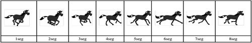
The task is to recognize the pattern shown in Figure 1. It is assumed that the pattern consists of a sequence of discrete images recorded in 8 sec, one per second.

Figure 1. Galloping horse.

In this case study, the recognition by perception is analyzed. At the level of perception, we have the following DpoP: the tail, the legs, the body, and the head. The dynamic of this pattern (horse) is guided by changes in function of the horse’s dynamic stance defined by the descriptors mentioned. Suppose the Eq. (1), ρ_d=horse = < D_n, f_Δ, Δτ>.

Using Eq. (2), the vector D_n with the collection of all the n descriptors DpoP of ρ_d=horse is:

Now, the Eq. (4) is . Remember is the domain vector of (y is the perception descriptor) and has a range of values from to , with y = 1,2,3… to an arbitrary value, depending on the domain. Each value represents a dynamic value. For example, for the descriptor of the tail, when will mean tail up, means tail straight, and means tail below. That is similar for the other descriptors.

The eight values in the leg in the descriptors represent the eight possible positions of the legs, which can be described in different ways, for example, by internal angles, its distance to the body, its shape; for example, leg stretched, =2 = leg collected, etc.

Additionally, the change functions are defined. These functions model the transition (possible change) of the values of each descriptor (according to theirs domains). We define a change function for each descriptor.

Finally, each one of the descriptors may have a different time rate of change.

Remember, we want to recognize the galloping horse of the Figure 1. The recognition should be given in any of the eight times, which would result in “I’m seeing a horse gallop”.

To continue, we analyze the last two top levels of the hierarchy (see Figure 2): at the level X_a we have Γ_ja modules for the pattern recognition of parts of an animal (LegRightD,LegLftD, LegRightT, LegLeftT, Tail, Body, Head), and level X_u, modules for the pattern recognition of an animal (such as horse, cow).

Figure 2. Three levels of the hierarchy of patterns, to recognize the pattern “horse”.

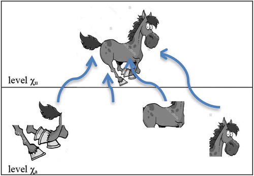
Now, we execute our general recognition algorithm (see AR2P algorithm in Puerto and Aguilar (2016b)). The process receives as input y = s() = “the image of the horse in the first second”. A decomposition of the image is then performed in its subpatterns < LegRightD,LegLftD, LegRightT, LegLeftT, Tail, Body, Head>. Then, it is determined the X_i level of the hierarchy where the process begins the recognition of (y), in this case X_i=2 (level of the animals).

At this level (X_i = X_u), their modules are instantiated for each instant of time. For example, the Table 2 shows an instance of the data structure of the image “horse” corresponding to the first image (first second). Then, L requests of petition for recognition of y are created, <y1 = legRightD, y2 = LegLeftD, y3 = LeftRightT, y4 = LeftLeftT, y5 = body, y6 = tail, y7 = Head>, in the next level.

Table 2. Matrix E_d = < Galloping horse>.

Ed
Sd		Cd
Signal	State	Pointer (P)^a	Weight (W)
1 =	T	Pointer^1	0.9
2 =	T	Pointer^2	0.6
3 =	T	Pointer^3	0.6
4 =	T	Pointer^4	0.6
5 =	T	Pointer^5	0.6
6 =	T	Pointer^6	0.8
7 =	T	Pointer^7	0.9
Ud: < 0.85, 0.65 >

Assuming the patterns (tail, legleftD, lefRightD, …) were recognized at the level X_a, they change the states of the superior levels of the hierarchy (level X_u). This level receives these recognized signals, and calculates the recognition using the theorems proposed:

Let ΔU1 = 0.85, and that all signals were recognized (their status are “True”, see Table 2). Then, we can recognize by perception (DpoP) according to the Eqs. (11)-(13). According to Eq. (11), the key signals of this pattern are: signals 1, 6, and 7. Now, we use Eq. (13) to determine if the pattern can be recognized with these recognized signals. These signals are sufficient to overcome the threshold (0.86 > 0.85). Pattern recognition is successful, and because is the last level of the hierarchy X_u (the level where began the process of recognition), it produces the output signal S_o, and generates the system output signal: “S0 = I’m seeing a horse gallop”.

Recognition of the emotions “anger” or “happiness”, by dynamic patterns oriented to characteristics (DpoC)

In this case, we recognize the emotional patterns of a car driver using dynamic patterns oriented to characteristics (DpoC). We define three physiological descriptors with the value of the Table 3 for each emotion, in order to test the emotion recognition in our system: one for when the car driver is happy, and another for when the car driver is with anger.

Table 3. Physiological conditions for the emotional patterns of a car driver.

Physiological pattern of a car driver	Happy	Heart rate	From [0.1 to 0.4]
		Respiratory rate	From [0.1 to 0.4]
		Blood pressure	From [0.1 to 0.4]
	Anger	Heart rate	From [0.5 to 1.0]
		Respiratory rate	From [0.5 to 1.0]
		Blood pressure	From [0.5 to 1.0]

All values are normalized in [0, 1]. It is assumed that the pattern consists of a sequence of values (heart rate, respiratory rate, or blood pressure) of the emotional state of the car driver in a time interval Δt. Suppose the Eq. (1), Γ_{ρd= joy} = < D_n, f_Δ, Δτ>. Using Eq. (2), the vector D with the collection of all the n descriptors DpoC of Γ_ρd=happy is:

D_n(happy) = [d_hearate, d_{respiratorate}, d_{bloodpressure}] In the same way for Γρ_d=angry

Tables 4 and 5 show the structure of the recognition module for each emotion

Table 4. Matrix Γρ_{d = angry.}

Ed
Sd		Cd
Signal	State	Pointer (P)	Weight (W)
1	F	PointerAngry1hearate	1
2	F	PointerAngry2respitarotate	0.8
3	F	PointerAngry3bloodpressure	0.9
Ud: <ΔU1, ΔU2 >

Table 5. Matrix Γρ_{d = happy.}

Ed
Sd		Cd
Signal	State	Pointer (P)	Weight (W)
1	F	PointerHappy1hearate	0.8
2	F	PointerHappy2respitatorate	0.9
3	F	PointerHappy3bloodpressure	0.8
Ud: <ΔU1, ΔU2 >

To recognize a dynamic pattern, its descriptors are evaluated in a time interval [t_i=1, t_j=n]. Suppose the next time series for Anger (see Eq. (6)).

And for happy.

Suppose the next input s() = {hearate[(t1, 0.5),(t2, 0.6),(t3, 0.7), (t4, 0.8)], respiratorate[(t1, 0.5),(t2, 0.5),(t3, 0.6),(t4, 0.8)], bloodpressure[(t1, 0.5),(t2, 0.6),(t3, 0.7),(t4, 0.7)]} from a car driver.

Each element of this set is an atomic input pattern. Each pattern is recognized individually, through a direct mapping to the existing set of time series (via the pointer). Of the three patterns, only hearate is recognized, which match the pattern of heart rate of the anger emotion. This causes a change in the first signal of the recognition module of anger, of false to true (see Table 6).

Table 6. Matrix Γρ_{d = angry.}

Ed
Sd		Cd
Signal	State	Pointer (P)	Weight (W)
1	F	PointerHappy1hearate	1
2	F	PointerHappy2respitatorate	0.9
3	F	PointerHappy3bloodpressure	0.8
Ud: <ΔU1, ΔU2 >

Let ΔU1 = 0.9. Then, we can recognize by characteristic (DpoC) according to the Eqs. (10–12). According to Eq. (10), the key signals of this pattern are the first and third signals. Now, we use Eq. (12) to determine if the pattern can be recognized with the recognized signals (first signal). These signals are sufficient to overcome the threshold (1 > 0.9). Pattern recognition is successful, and how it is the last level of the hierarchy X_u (the level where began the process of recognition), it produces the output signal S_o, that becomes in the system output signal: “S_o = angry”.

Conclusions

This paper presents a formal model for the dynamic and static pattern recognition, based on the theory of mind proposed in (Kurzweil 2012). The proposed model is a computational approach to pattern recognition based on the functional mechanisms of the human brain.

Our pattern recognition model is highly recursive and uniform. The uniformity allows the recursive process to be the same in all the levels. Thus, the model recognizes a pattern of input no matter their level of complexity or the nature of the same (static or dynamic). The model recognizes the input patterns by a process of self-association in a pattern hierarchy.

The model can recognize a dynamic pattern from two major orientations: recognition of dynamic patterns oriented by characteristics, or by perceptions. In addition, the model uses two strategies for recognition; one for key signals and another for total or partial mapping. The first exploits the important signals that facilitate the recognition; the second strategy completely exploits the input signals. In the key signal strategy, it can predict a pattern even with missing information.

Another important feature of the model that makes it different from other recognition systems is its ability to recognize a pattern using the natural dynamic of the pattern. Specifically, it uses time series and automata for that.

At the computational level, the proposed model offers a concise, readable and elegant solution (recursivity), but it defines a tree, which can be very large. One possible optimization is to use parallelism to improve the execution time. Additionally, a main problem is to define the atomic level for each pattern. Future works will be dedicated to extend this model considering both aspects has not been published elsewhere and that it has not been submitted simultaneously for publication elsewhere. Finally, we state that this manuscript has not been published elsewhere and that it has not been submitted simultaneously for publication elsewhere.

Acknowledgments

Dr Aguilar has been partially supported by the Prometeo Project of the Ministry of Higher Education, Science, Technology and Innovation of the Republic of Ecuador.

References

- Aguilar, J. 2004. A color pattern recognition problem based on the multiple classes random neural network model. Neurocomputing 61:71–83.
- Aguilar, J., and A. Colmenares. 1997. Recognition algorithm using evolutionary learning on the random neural networks. In IEEE International Conference on Neural Networks, vol. 2, pp. 1023–28. Houston, USA.
- Alpaydin, E. 2014. Introduction to machine learning. Cambridge, England: MIT press.
- Bobrow, J. 2014. Representation and understanding: Studies in cognitive science. New York, USA: Elsevier.
- Felzenszwalb, P., D. McAllester, and D. Ramanan. 2008, June. A discriminatively trained, multiscale, deformable part model. Computer Vision and Pattern Recognition, 2008. CVPR 2008. IEEE Conference on (pp. 1–8). Anchorage, USA: IEEE.
- Hawkins, J., and S. Blakeslee. 2007. On intelligence. New York, USA: Macmillan.
- Kaku, M. 2014. El futuro de nuestra mente. Barcelona: Debate.
- Kelso, J. S. 2014. The dynamic brain in action: Coordinative structures, criticality and coordination dynamics. In Criticality in Neural Systems, ed. D. Plenz and E. Niebur, 67–104. Berlin, Germany: Wiley.
- Kurzweil, R. 2012. How to create a mind: The secret of human thought revealed. New York, USA: Penguin.
- LeCun, Y., Y. Bengio, and G. Hinton. 2015. Deep learning. Nature 521 (7553):436–44.
- Liu, C., B. Lovell, D. Tao, and M. Tistarelli. 2016. Pattern recognition, part 1. in: IEEE Intelligence Systems. IEEE 31 (2):6–8.
- Lopes, N., and Ribeiro, B. 2015. Machine Learning for Adaptive Many-Core Machines-A Practical Approach. New York, USA: Springer International Publishing.
- Markram, H. 2012. The human brain project. Scientific American 306 (6):50–55.
- Moser, M. B., and E. I. Moser. 2014. Understanding the Cortex through Grid Cells. In The future of the brain: Essays by the world’s leading neuroscientists. ed. G. Marcus, and J. Freeman, 67–77. New Jersy, USA: Princeton University Press.
- National Institutes of Health. The brain initiative, US. Accessed October 8, 2016. hhttp://www.braininitiative.nih.gov/2025/index.htm.
- Pavlidis, T. 2013. Structural pattern recognition, Vol. 1. Berlin, Germany: Springer.
- Puerto Cuadros, E. G., and J. L. Aguilar Castro. 2016a. Learning algorithm for the recursive pattern recognition model. Applied Artificial Intelligence 30 (7):662–78.
- Puerto, E., and J. Aguilar. 2016b. Formal description of a pattern for a recursive process of recognition. Computational Intelligence (LA-CCI), 2016 IEEE Latin American Conference on. pp. 1–2. Cartagena, Colombia.
- Srivastava, N., R. R. Salakhutdinov, and G. E. Hinton. 2013. Modeling documents with deep boltzmann machines, Twenty-Ninth Conference on Uncertainty in Artificial Intelligence, pp. 616–624. Arlington, USA.
- Taubman, D., and M. Marcellin. 2012. JPEG2000 image compression fundamentals, standards and practice. New York, USA: Springer.
- Watanabe, S., Ed. 2014. Methodologies of pattern recognition. New York, USA: Academic Press.
- Xu, T., Z. Yang, L. Jiang, X. X. Xing, and X. N. Zuo. 2015. A connectome computation system for discovery science of brain. Science Bulletin 60 (1):86–95.