Recurrent Neural Network to Forecast Sprint Performance

ABSTRACT

The present paper demonstrates that the performance of an elite track and field sprinter can be predicted by means of the dynamic, nonlinear mathematical method of recurrent neural networks (RNNs). Dataset considers three years of National Collegiate Athletics Association (NCAA) Division I competitions where the student-athlete recorded heart rate variability two days precedent to each competition. Input parameters were selected by transfer entropy via permutation tests. Subsequently, two RNN topologies, Elman and Jordan, were trained with 32 competitions, validated with 7 competitions, and tested against 6 held-out competitions. Resultant RNNs, which possess a sense of time and memory, were able to learn time-dependent sequence of acute adaptation and predict race times with an error of 0.09–0.16 s on held-out test data. Root mean sum of differences of successive R-R intervals (RMSSD), an indicator of parasympathetic tone, and direct current biopotentials, indicator of active wakefulness, were most predictive toward competitive performance for an NCAA Division I male sprinter.

Introduction

Sprinting performance, as with most individual sports, is more closely connected to acute physiological readiness in comparison to the complexity of team sport success. Consistent analysis of objective, internal athlete monitoring can depict an athlete’s undulating physiological readiness in response to external training stimuli (Halson 2014). Although coaches utilize this information to examine retrospective adaptive behavior to augment the training management process, there is potential for predictive methods that have largely gone unnoticed for the preparation of competitions.

A common athlete monitoring tool to provide indication of physiological readiness is heart rate variability (HRV). Beat-to-beat variability of the heart is reflective of autonomic balance, which sport practitioners exploit in an effort to delineate an organism’s adaptive capabilities (Buchheit 2014). For example, increases in sympathetic tone are suggestive of early signs of overreaching, whereas extended periods of overreaching can be expressed by parasympathetic dominance (Lehmann et al. 1998). HRV has traditionally been a tool for monitoring aerobic-dominant sports (Buchheit 2014), but it has recently been a developing area of research for the applicability for intermittent, team-based sports performance, such as basketball (Fronso et al. 2012), Australian football (Cornforth et al. 2015), and badminton (Bisschoff et al. 2018). However, HRV for anaerobic neuromuscular performance remains relatively unexplored (Buchheit 2014).

Another biological proxy that has influenced the sport fraternity is the estimated functional state of the central nervous system (CNS) via direct current biopotentials (DC Potential). Ilyukhina (1982) presented a noninvasive approach to quantify the excitability of underlying cortical tissue via DC potential, termed omegametry. DC potential was able to recognize alterations in CNS states, such as exhaustion or tension, and was suggested that DC potential could detect changes in an athlete’s functional state (Ilyukhina et al. 1982). Unfortunately, empirical evidence substantiating omegametry with athletic performance in competitive environments remains embryonic, leaving coaches to infer from raw data with little guidance. More recently, Morris (2015) evaluated physiological readiness with elite anaerobic athletes via HRV and omegametry. The results illustrated improved adaptations in power expression when HRV and omegametry guided the training versus a control group whose training was not altered. However, this study, albeit invaluable, refrained from evaluating competitive athletic environments and relied on linear methodology for analysis.

Linear methods fall short when modeling human performance from variables that characterize nonlinear biological systems (De’arth and Fabricius 2000) and is obligatory for models to be dynamic in order to appreciate how systems evolve over time (Cook 2016). Such propositions invite researchers to explore the utility of more sophisticated modeling strategies to forecast human performance. Edelmann-Nusser, Hohmann, and Henneberg (2002) is an example of such nonlinear methodology, who successfully predicted an Olympic swimmer’s performance via artificial neural networks. Although their progressive efforts are sincerely applauded, this study used time-lagged external load parameters as inputs to a time-independent (static) network architecture and was therefore not dynamic. The authors highlight that the error of the particular Olympic competition was 0.05 s, but the overall model performance exhibited an error of 1.23 s, which is hypothesized to shrink when appropriately incorporating the element of time to the neural network framework. Recurrent neural network (RNN) architecture, which adds a sense of memory to the network, is the sequential (temporal) counterpart to standard neural networks seen in Edelmann-Nusser, Hohmann, and Henneberg (2002). Therefore, the purpose of the present study is to dynamically forecast elite track and field sprint performance by proper inclusion of time via RNNs. Alternatively, the present study uses HRV and omegametry as input parameters in order to forecast performance based on how the athlete’s biological readiness evolves over time.

Methods

Dataset

Retrospective case study was employed to assemble dataset. One male Division I National Collegiate Athletics Association (NCAA) track and field student-athlete voluntarily monitored HRV (Omegawave Oy, Espoo, Finland) throughout his competitive career as a part of routine health and well-being surveillance. Student-athlete competed in 60 m hurdles (indoor) and 110 m hurdles (outdoor). Final race times and competition dates are undisclosed to protect confidentiality. The present study conforms to the ethical standards of the Helsinki Declaration.

In order for competition to be considered in dataset, three consecutive HRV measurements were completed within two calendar days leading into competitive event (two days prior: t-2, day before: t-1, morning of: t) where he successfully recorded a final race time (t). Conclusive dataset was randomly partitioned into three segments: 32 competitions (71%) for training, 7 competitions (16%) for validation, and 6 competitions (13%) set aside for terminal evaluation.

HRV and omegametry procedures

Omegawave technology allows comprehensive analysis of HRV and direct current biopotentials through a number of linear and nonlinear techniques. Student-athlete was issued an Omegawave heart rate strap which was adjusted according to his respective chest size. Upon moistening with tap water, student-athlete tied the heart rate strap around his torso at the level of his xiphoid process ensuring that the electrocardiogram pads were aligned with his midaxillary line. DC potential was noninvasively recorded by means of small portable DC-amplifiers connected to the frontal eminence of his scalp and thenar eminence of his right hand. To ensure reliable measurements, student-athlete performed assessments antemeridian (between the hours of 06:00 and 08:00) in a rested state while lying supine in a room with minimal light and distraction. Duration of assessments was 4 min in length to obtain time- and frequency-domain HRV indices and allow ample time for omegametry to stabilize. Table 1 provides a glossary of numerical HRV and omegametry parameters provided by Omegawave.

Table 1. Glossary of numeric HRV and omegametry parameters.

Name	Abbreviation	Scale	Units	Interpretation
Adaptation reserve ^†	AR	O	Scale (1–7)	Reflects how long cardiac system can express adaptability.
Aerobic index^†	Aerobic	I	N/A	Reflects state of aerobic metabolic pathways.
Anaerobic index^†	Anaerobic	I	N/A	Reflects state of anaerobic metabolic pathways.
Central nervous system readiness ^†	CNS	O	Scale (1–7)	Comprehensive indicator of central nervous system readiness.
Direct current potential^†	DC^‡	C	mV	Present activation of frontal brain system. Reflects wakefulness.
Fatigue index ^†	Fatigue	O	Scale (1–7)	Reflects temporary state of cardiac system.
Heart rate at anaerobic threshold	HR AN	I	bpm	Overall indicator of endurance level.
High frequency	HF*^‡	C	ms^2	Power in high-frequency range. Reflects parasympathetic activity.
High-frequency normalized units	HF nu	C	N/A	High-frequency power in normalized units.
Low frequency^†	LF*	C	ms^2	Power in low-frequency range. Reflects parasympathetic activity.
Low-frequency normalized units	LF nu	C	N/A	Low-frequency power in normalized units.
Low-frequency/high-frequency ratio	LF/HF*	R	N/A	Reflect sympathetic–parasympathetic balance.
Metabolic grade ^†	Metabolic	O	Scale (1–7)	Comprehensive indicator of metabolic system coordination.
Metabolic reactive index ^†	MRI*	C	N/A	Estimate of overall coordination of metabolic systems.
Parasympathetic activity ^†	PNS	C	s	Indicator of current level of parasympathetic nervous system regulation.
Root mean sum of differences of successive intervals	RMSSD*^‡	C	ms	Square root of sum of difference of sequential cardio intervals. Reflects autonomic activity.
Share of aperiodic influences	AI	C	s	Reflects level of random activity that influences heart rhythm.
Standard deviation of aspirate waves	SDAW*	C	N/A	Reflects level of automatization of heart rhythm regulation.
Standard deviation of normal-to-normal intervals	SDNN*	C	ms	Reflects autonomic regulation from full array of cardio intervals.
Standard deviation of successive differences	SDSD*	C	ms	Standard deviation of differences between adjacent intervals.
Stress index ^†	Stress	O	Scale (1–7)	Level of tension in cardiac system.
Sympathetic activity ^†	SNS	C	%	Indicator of current level of sympathetic nervous system regulation.
Tension index ^†	TI*	C	N/A	Reflects level of centralization of heart rhythm regulation.
Total power	TP*^‡	C	ms^2	Variance of all intervals to reflect level of regulatory system.

C = continuous; I = interval; O = ordinal; R = ratio.

*Log-transformation applied to address positive skewness.

^†Denotes proprietary Omegawave parameter.

^‡Variable selected from ordered lasso regularization.

Preprocessing and feature selection

Germane data preprocessing was performed prior to modeling procedures. Shapiro–Wilk test was applied to all features, which were appropriately transformed when significance was encountered (denoted in Table 1). Subsequently, all features were linearly transformed to normalize distance: Henceforth, race times are kept on normalized scale (0 = fastest, 1 = slowest) and are therefore expressed as normalized units (nu).

With 24 candidate predictors, dimension reduction was performed with the objective of establishing a subset of input variables that parsimoniously affect output variable in a temporal fashion. However, feature selection directly from RNNs has yet to be fully elucidated due to the complex arrangement of weights (Guo, Lin, and Lu 2018), and therefore, a model-agnostic feature selection approach was implemented precedent to RNN development. Thus, with the training dataset, transfer entropy (TE) was calculated between each candidate predictor and race time to identify the strength of interdependence within the multivariate time series. TE, an asymmetric (directional) information-theoretic measure, has popularized in time series feature selection (Mao and Shang 2017) from its effectiveness to detect nonlinear, temporal dependencies via transitive probabilities (Schreiber 2000). As suggested by Gomez-Herrero et al. (2015), statistical significance of TE was assessed via permutation test with surrogate data generated by randomly shuffled trials (5000 permutations each). Features were thus selected for RNN inputs when permutation tests deemed significant (p < 0.05).

Network topologies

RNNs are a division of feedforward neural networks enhanced by nodes that connect back to other nodes, allowing the activation of nodes to flow in a loop (Hochreiter and Schmidhuber 1997). Therefore, unlike standard multi-layer perceptrons, RNN architecture has a sense of time and memory of earlier network states which enables it to learn sequences that vary over time (Cruse 2006). At time step t, nodes receive input activation from current instance x^(t) as well as from hidden node h^(t−1) in network’s former state (Haykin 2009; Lipton, Berkowitz, and Elkan 2015). Output ^(t) is calculated given the hidden state h^(t) at respective time step. Thus, input x^(t−1) at time step t-1 can impact output ^(t) at time step t by means of these recurrent connections (Lipton, Berkowitz, and Elkan 2015).

Calculations for computing each time step in RNN are as follows:

where the sigmoid () represents the respective activation function, symbolizes the matrix of weights between input and hidden layers, and symbolizes the matrix of recurrent weights between hidden layers at adjacent time steps. Vectors and are biases which allow individual nodes to learn an offset (Lipton, Berkowitz, and Elkan 2015).

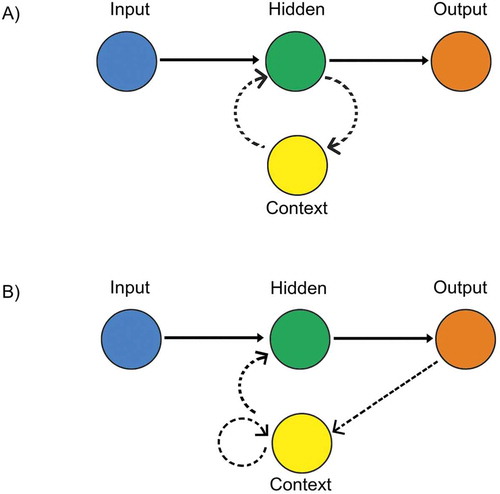
The two RNN topologies explored, Elman and Jordan, represent a general format for RNN development. Elman recurrent neural networks (ERNNs) provide a model with an input layer, a hidden layer, and an output layer connected in a feedforward manner (Elman 1990). However, the hidden layer is also connected to a further layer called the context layer (Figure 1(a)). This recurrent connection of the context layer provides the model with a short-term memory; the hidden nodes are influenced by input nodes while obtaining information of their former state via their context node (Elman 1990). Thereby, the model learns to attribute an output directly from the temporal sequence of several subsequent input vectors. Jordan recurrent neural networks (JRNNs) propose a similar model, but the induction of memory states is from the context nodes being fed from the output layer (Figure 1(b)), rather than the hidden layer (Jordan 1997). That is, a constant input vector is given to the network, which the output layer then performs the temporal sequence of vectors (Jordan 1997).

Figure 1. Sample RNN topologies: (a) Elman and (b) Jordan.

Model construction and evaluation

Features were transposed prior to training to properly invoke temporal sequence preceding competitive event. Initial ERNN learning rate was set at 0.10, and the number of training epochs was set to 100. Model complexity was manipulated by adjusting the number of hidden layers and nodes per hidden layer. Training iterations (by tuning learning rate, epochs, layers, and nodes per layer) were performed on validation set until most optimum error was realized. JRNN began with same tuning parameters; however, JRNN only allows one hidden layer (Jordan 1997). Therefore, model complexity was simply adjusted by incrementally increasing the number of hidden nodes. Once optimal tuning parameters were determined, respective models were placed in production to test against held-out dataset.

To justly compare the time series prediction capability of RNN topologies, a competitive time series regression equipped for dynamic systems (Keele and Kelly 2006) was also calculated from training dataset as a separate analysis. An ordered lasso (Tibshirani and Sou 2016) applied to a two-step time-lagged regression was the chosen statistical model for two reasons: (1) to leverage the feature selection property of ℓ₁-regularized regression (Tibshirani 1996) and (2) to preserve the temporal structure of original data.

To quantitatively evaluate the performance of all three models, two error statistics were calculated: mean bias error (MBE) and root mean square error (RMSE). MBE denotes average direction of estimate deviation from true measured data (Stone 1993). In the present context, positive MBE indicates magnitude of underestimation in predicted race times (due to minimization objective of racing), whereas negative MBE indicates overestimation of sprint performance. On the other hand, RMSE presents information of model performance via an average measurement of variation in predicting the dependent variable (Hyndman and Koehler 2006). Therefore, RMSE exhibits the efficiency of trained model in predicting the future individual races. To determine whether a model’s estimates were statistically significant, the t-statistic was derived from RMSE and MBE (Stone 1993). Performance indices were calculated as:

where is predicted race time, is true race time, and n is number of instances. To be judged statistically significant, respective t-statistics were to be smaller than t critical value (df = 5, α = 0.05; t_crit = 2.02).

To aid the comprehension of resultant RNNs, individual conditional expectation (ICE) plots were computed to approximate the functional relationship between race time and most predictive features (Goldstein et al. 2015). ICE plots, an extension of Friedman’s (2001) partial dependence plots, unveil the estimated distribution of n observations against the response function. Thus, ICE plots elucidate the variants of conditional relationships estimated by statistical learning algorithm (Goldstein et al. 2015). To help discern heterogeneity between curves, ICE plots were centered at the minimum value of predictor variable to account for differing intercepts. Additionally, partial derivatives of the model were plotted to highlight the location and magnitude of hypothesized interaction effects. Hereafter, ICE plots will be labeled c-ICE for centered and d-ICE for partial derivative.

RStudio software (version 1.0.143) was used for all outlined statistical procedures.

Results

Resultant subset of variables with non-zero coefficients from time-lagged ordered lasso (TLOL) constraint is indicated in Table 1. Upon validation iterations, TLOL converged with a lambda of 5.75, resulting in four non-zero coefficients remaining. TLOL training performance concluded with RMSE = 0.21 normalized units (nu).

RNN feature subset from TE reduced the dimensions from 24 to 9 variables, as outlined in Table 2. Final ERNN model parameters from validation set arrived at a learning rate of 0.15, 500 training epochs, and 3 hidden layers with 12, 10, and 7 nodes per layer, respectively, achieving optimal RMSE = 0.06 nu. Final JRNN model parameters from validation set arrived at a learning rate of 0.20, 300 training epochs, with 17 nodes in hidden layer, converged at RMSE = 0.04 nu.

Table 2. Pairwise transfer entropy (TE) against race time with permutation p-values.

Candidate feature	TE (bits)	p
RMSSD*	0.37	<0.001
DC*	0.31	<0.001
SDSD*	0.27	0.004
SDNN*	0.26	0.009
SDAW*	0.26	0.012
HF*	0.22	0.028
TP*	0.19	0.034
SNS*	0.19	0.036
LF*	0.17	0.041
TI	0.09	0.089
AI	0.09	0.116
Aerobic	0.07	0.220
HR AN	0.06	0.394
MRI	0.06	0.406
PNS	0.04	0.434
CNS	0.04	0.456
Stress	0.03	0.482
LF nu	0.03	0.488
HF nu	0.03	0.494
LF/HF	0.02	0.530
Metabolic	0.02	0.592
Anaerobic	0.02	0.622
AR	0.02	0.651
Fatigue	0.01	0.870

*Selected feature from permutation significance.

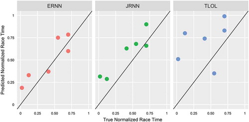
Against terminal, held-out test data, TLOL regression model generated an accuracy of RMSE = 0.38 nu, MBE = 0.28 nu, and t = 2.44 and ERNN model generated an accuracy of RMSE = 0.14 nu, MBE = 0.09 nu, and t = 1.63, whereas JRNN generated an accuracy of RMSE = 0.19 nu, MBE = 0.16 nu, and t = 3.49. Figure 2 illustrates raw prediction performance against true measurement data on normalized scale for each respective model. After race times were back-transformed, TLOL error for the 60 m hurdles corresponds to RMSE = 0.24 s and MBE = 0.17 s, whereas for the 110 m hurdles RMSE = 0.32 s and MBE = 0.23 s. ERNN error for the 60 m hurdles corresponds to RMSE = 0.09 s and MBE = 0.05 s, whereas for the 110 m hurdles RMSE = 0.12 s and MBE = 0.07 s. JRNN error for the 60 m hurdles corresponds to RMSE = 0.12 s and MBE = 0.10 s, whereas for the 110 m hurdles RMSE = 0.16 s and MBE = 0.13 s.

Figure 2. Terminal model accuracies against held-out test data. Solid black line indicates perfect prediction.

Discussion

Results demonstrate that RNN framework was excellent at predicting elite sprint performance on the basis of temporal HRV measurements. The vast error improvement in both training and testing compared to TLOL regression showcases that the mechanics of neural memory were superior to regularized autoregressive ordinary least squares when modeling adaptive behavior. TLOL was able to mildly forecast performance in the correct direction but witnessed large deviations from the true absolute observations (vertical distance from diagonal line), whereas RNN topologies were able to learn the correct direction with relative precision. Therefore, from a synergistic point of view, a successful RNN crafted from biological indices may be representative of self-organizing systemic deviations that influence certain states of stable performance.

Between the two RNNs, it is of interest that JRNN slightly outperformed ERNN amid validation process but fell behind when tested against held-out data. Perhaps, JRNN overfit the validation set with too many hidden nodes, which weakened the applicability to future instances. The multiple hidden layers permitted by ERNN may have composed a proficient topology to learn the underlying concept more advantageously. Though the mechanism for the current ERNN dominance is unclear, ERNN would be the chosen model to place in production for the present scenario, given the statistically significant performance over JRNN.

To extrapolate the hypothesized feature space constructed by the network, Figures 3 and 4 display the ICE plots from conclusive ERNN model, stratified by time, of the two most predictive features found from transfer entropy. Starting with c-ICE plot in Figure 3, the universal effect of the natural log (ln) RMSSD is a positive trend, indicating that, on average, higher ln-RMSSD values were associated with higher (slower) fitted race times. It is apparent that, in general, effects seem to amplify when closer in chronological proximity to event; ln-RMSSD t-2 exhibits moderately noisy effects, whereas the functional relationship of t-1 and t seems to sharpen with more pronounced interactions.

Figure 3. ERNN c-ICE and d-ICE plots of ln-RMSSD stratified by time.

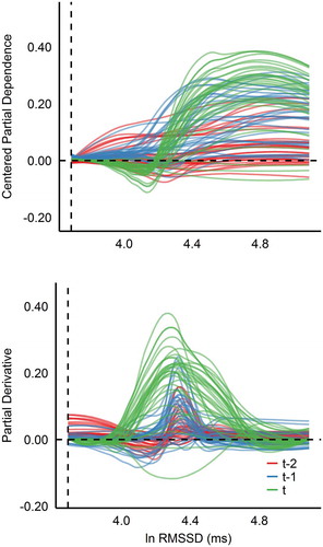
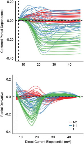
Figure 4. ERNN c-ICE and d-ICE plots of DC stratified by time.

When observing the shape and direction of individual curves from left to right, ln-RMSSD t-1 and t express a stable system in the first third of the range, with perhaps a slight decrease (positive) effect in t. Beyond this point is where the cumulative effect of ln-RMSSD begins to negatively influence race times. This suggests that the sprinter’s athletic performance was generally unaffected until ln-RMSSD values were above roughly 4.4 ms, with the effect of adding nearly 0.4 normalized units to the fitted race time, when considering ln-RMSSD t independently. That is, the athlete experienced performance decrements when his autonomic nervous system expressed parasympathetic dominance. Examining the d-ICE plot in the bottom half of Figure 3 confirms the observations made above, casting light on the region of interaction around 4.4 ms. A secondary, but weaker, inference is that his most desirable ln-RMSSD range was potentially 4.0–4.2 ms. Overall, these phenomena indicate that the predictive power of ln-RMSSD toward sprint performance primarily manifested in a negative fashion. It was essential for ln-RMSSD to reflect more balanced autonomic regulation the morning of competition, perhaps to allow greater acquisition of maximal sympathetic mobilization at race time (Hedlin, Bjerle, and Henriksson-Larsen 2001).

Shifting to DC Potential in Figure 4 seems to share similar properties regarding chronological magnification, but stability conversely arises in second half of DC’s range, which is clearly demonstrated from the partial derivatives. From right to left, fitted race times are generally unaffected until roughly 20 mV where interactions begin. Although heterogeneity exists between curves in t-1, a positive quadratic functional relationship presents itself between 20 and 30 mV. This local minimum indicates most ideal DC range for the sprinter the day prior to a given competition. Whereas on the day of competition (t), race times were only affected (negatively) when below 20 mV, also suggesting optimal performance was more likely when above 20 mV.

Ilyukhina (2013) physiologically substantiates low DC biopotentials (< 20 mV) as the CNS exhibits attenuated levels of active wakefulness, suggesting that this range may indirectly estimate adaptive limitations of central regulatory systems and decreased functional reserves. Ilyukhina and Zabolotskikh (2000) demonstrated that individuals who express resting biopotentials < 23 mV were less resilient to physical exertion compared to individuals with elevated values. Although the participants in Ilyukhina and Zabolotskikh (2000) were not elite sprinters, it is worth emphasizing that the RNN in the present analysis inductively detected a performance threshold parallel to prior DC literature.

Considering the relative variable importance in Table 2, among the numerous HRV candidate variables, it appears that raw time domain indices were generally more predictive compared to other meta-variables for the particular athlete. This coincides with recommendations given by Buchheit (2014), in that practitioners in the field should perhaps select parameters that are more likely to directly reflect parasympathetic activity.

In practice, models trained per individual not only could predict approaching competitions but may also serve as a simulation tool for estimating prospective athletic performances when under differing physiological states. Thus, a trained RNN may help coaches optimize athlete training by enabling them to forecast physical aptitude prior to a given training session. If perhaps a large discrepancy arises between an athlete’s estimated physical capacity and a coach’s planned expectation, appropriate modifications could be made in order to dovetail the training plan with the athlete’s readiness, if desired.

Limitations

An apparent limitation of the present analysis is due to the sole incorporation of internal parameters for model prediction. External training loads, which inherently influences autonomic balance (Buchheit 2014; Halson 2014), were not recorded and thus were unable to be included. Integrating more diverse features (external training loads, environmental conditions, etc.) could perhaps ameliorate predictive accuracy in future models.

It is also worth noting the innate limitation of the study design. While case studies yield rich investigations, their granularity is offset by unsatisfactory generalizability. Therefore, the precise order of relative importance of HRV parameters, and the functional relationships portrayed in ICE plots, may not hold true for different athletes. Thus, readers are encouraged to abstract the utility of aforementioned modeling procedures for athletic performance prediction rather than gleaning individual physiological constructs.

Conclusion

RNN infrastructure was used as a computational device to recognize adaptive states that lead to athletic performance. ERNN model outperformed JRNN against held-out test data, resulting in an error of 0.09–0.12 s and 0.12–16 s, respectively. RMSSD, an indicator of parasympathetic tone, and direct current biopotentials, indicator of active wakefulness, were most predictive toward competitive performance for an NCAA Division I male sprinter. Future investigations could explore modeling how internal readiness is influenced by external training patterns and lifestyle habits leading up to competition, as well as incorporating subjective readiness parameters.

Conflict of Interest

No conflict of interest present. The author declares zero affiliation with Omegawave Oy.

Acknowledgments

The author would like to express sincere gratitude to the University of Iowa Athletic Department for their support. A special thanks is also sent to the student-athlete for his relentless dedication. The author would also like to thank the anonymous reviewers for taking time to improve this manuscript.

References

- Bischoff, C. A., B. Coetzee, and M. R. Esco. 2018. Heart rate variability and recovery as predictors of elite, African, male badminton players’ performance levels. International Journal of Performance Analysis in Sport 18 (1):1–16. doi:10.1080/24748668.2018.1437868.
- Buchheit, M. 2014. Monitoring training status with HR measures: Do all roads lead to Rome? Frontiers in Physiology 5:1–19. doi:10.3389/fphys.2014.00001.
- Cook, C. 2016. Predicting future physical injury in sports: It’s a complicated dynamic system. British Journal of Sports Medicine 50:1356–57. doi:10.1136/bjsports-2016-096445.
- Cornforth, D., P. Campbell, K. Nesbitt, D. Robinson, and H. F. Jelinek. 2015. Prediction of game performance in Australian football using heart rate variability measures. International Journal of Signal and Imaging Systems Engineering 8 (1–2):80–88. doi:10.1504/IJSISE.2015.067072.
- Cruse, H. 2006. Neural networks as cybernetic systems. Bielefeld. Germany: Brains, Minds, and Media.
- De’arth, G., and K. E. Fabricius. 2000. Classification and regression trees: A powerful yet simple technique for ecological data analysis. Ecology 81:3178–92. doi:10.1890/0012-9658(2000)081[3178:CARTAP]2.0.CO;2.
- Edelmann-Nusser, J., H. Hohmann, and B. Henneberg. 2002. Modeling and prediction of competitive performance in swimming upon neural networks. European Journal of Sport Science 2 (2):1–10. doi:10.1080/17461390200072201.
- Elman, J. L. 1990. Finding structure in time. Cognitive Science 14:179–211. doi:10.1207/s15516709cog1402_1.
- Friedman, J. H. 2001. Greedy function approximation: A gradient boosting machine. The Annals of Statistics 29 (5):1189–232. doi:10.1214/aos/1013203451.
- Fronso, S., G. Delia, C. Robazza, L. Bortoli, and M. Bertollo. 2012. Relationship between performance and heart rate variability in amateur basketball players during playoffs. Sport Science & Health 8:45.
- Goldstein, A., A. Kapelner, J. Bleich, and E. Pitkin. 2015. Peeking inside the black box: Visualizing statistical learning with plots of individual conditional expectation. Journal of Computational and Graphical Statistics 24 (1):44–65. doi:10.1080/10618600.2014.907095.
- Gomez-Herrerro, G., W. Wu, K. Rutanen, M. C. Soriano, G. Pipa, and R. Vicente. 2015. Assessing coupling dynamics from an ensemble of time series. Entropy 17:1958–70. doi:10.3390/e17041958.
- Guo, T., T. Lin, and Y. Lu 2018. An interpretable LSTM neural network for autoregressive exogenous model, arXiv preprint arXiv:1804.05251.
- Halson, S. L. 2014. Monitoring training load to understand fatigue in athletes. Sports Medicine 44 (2):139–47. doi:10.1007/s40279-014-0253-z.
- Haykin, S. 2009. Neural networks and learning machines. 3rd ed. Upper Saddle River, NL: Pearson.
- Hedlin, R., P. Bjerle, and K. Henriksson-Larsen. 2001. Heart rate variability in athletes: Relationship with central and peripheral performance. Medicine and Science in Sports and Exercise 33:1394–98.
- Hochreiter, S., and J. Schmidhuber. 1997. Long short-term memory. Neural Computation 9 (8):1735–80.
- Hyndman, R. J., and A. B. Koehler. 2006. Another look at measures of forecast accuracy. International Journal of Forecasting 22 (4):679–88. doi:10.1016/j.ijforecast.2006.03.001.
- Ilyukhina, V. A. 1982. The omega potential: A quantitative parameter of the state of brain structures and organism. I. Physiological significance of the omega potential when recorded from deep structures and from the scalp. Human Physiology 8 (3):221–26.
- Ilyukhina, V. A. 2013. Ultraslow information control systems in the integration of life activity processes in the brain and body. Human Physiology 39 (3):323–33. doi:10.1134/S0362119713030092.
- Ilyukhina, V. A., A. Sychev, N. Shcherbakova, G. Baryshev, and V. Denisova. 1982. The omega-potential: A quantitative parameter of the state of brain structures and of the individual: II. Possibilities and limitations of the use of the omega-potential for rapid assessment of the state of the individual. Human Physiology 8 (5):328–39.
- Ilyukhina, V. A., and I. B. Zabolotskikh. 2000. Physiological basis of differences in the body tolerance to submaximal physical load capacity in healthy young individuals. Human Physiology 26 (3):330–36. doi:10.1007/BF02760195.
- Jordan, M. 1997. Serial order: A parallel distributed processing approach. Advances in Psychology 121:471–95.
- Keel, L., and N. J. Kelly. 2006. Dynamic models for dynamic theory: The ins and outs of lagged dependent variables. Political Analysis 14:186–205. doi:10.1093/pan/mpj006.
- Lehmann, M., C. Foster, H. H. Dickhuth, and U. Gastmann. 1998. Autonomic imbalance hypothesis and overtraining syndrome. Medicine and Science in Sports and Exercise 30 (7):1140–45.
- Lipton, Z. C., C. Berkowitz, and C. Elkan 2015. A critical review of recurrent neural networks for sequence learning, arXiv preprint arXiv:1506.00019.
- Mao, X., and P. Shang. 2017. Transfer entropy between multivariate time series. Communications in Nonlinear Science and Numerical Simulation 47:338–47. doi:10.1016/j.cnsns.2016.12.008.
- Morris, C. W. 2015. The effect of fluid periodization on athletic performance outcomes in American football players. PhD. diss., University of Kentucky.
- Schreiber, T. 2000. Measuring information transfer. Physical Review Letters 85:461–64. doi:10.1103/PhysRevLett.85.461.
- Stone, R. J. 1993. Improved statistical procedure for the evaluation of solar radiation estimation models. Solar Energy 51 (4):289–91. doi:10.1016/0038-092X(93)90124-7.
- Tibshirani, R. 1996. Regression shrinkage and selection via the lasso. Journal of the Royal Statistical Society, Series B 58:267–88.
- Tibshirani, R., and X. Sou. 2016. An ordered lasso and sparse time-lagged regression. Technometrics 54 (4):415–23. doi:10.1080/00401706.2015.1079245.