A Neuro-Genetic Technique for Pruning and Optimization of ANN Weights

ABSTRACT

A novel technique for optimization of artificial neural network (ANN) weights which combines pruning and Genetic Algorithm (GA) has been proposed. The technique first defines “relevance” of initialized weights in a statistical sense by introducing a coefficient of dominance for each weight and subsequently employing the concept of complexity penalty. Based upon complexity penalty for each weight, candidate solutions are initialized to participate in the Genetic optimization. The GA stage employs mean square error as the fitness function which is evaluated once for all candidate solutions by running the forward pass of backpropagation. Subsequent reproduction cycles generate fitter individuals and the GA is terminated after a small number of cycles. It has been observed that ANNs trained with GA optimized weights exhibit higher convergence, lower execution time, and higher success rate in the test phase. Furthermore, the proposed technique yields substantial reduction in computational resources.

Introduction

Artificial Neural Networks (ANNs) and genetic algorithms (GA) are popular paradigms for learning and optimization, each with their own strengths and weaknesses. ANNs trained with backpropagation (BP) algorithm are highly popular due to their low complexity and ease of implementation. However, they are prone to getting stuck in local minima thereby yielding suboptimal solutions. GA, on the other hand, is good at global search and exhibits a robust performance. Applications of GA have been reported for defense in biological and chemical warfare (Haupt and Haupt 2011), design of combinational logic (Louis 2005), and wireless ad-hoc networks (Karthikeyan, Baskar, and Alphones 2012). Recent advancements in GA is based on a three-dimensional cellular GAs proposed by Asmaa, Erdogan, and Arslan (2013) that provides better performance in terms of efficiency, and efficacy, for most of the problems. However, unguided mutation and variations in a host of parameters leads to extremely slow convergence of GA. With an aim to obtain complementary advantages from both GA and ANN, many researchers have reported a variety of neuro genetic techniques with varying success rates (Christiansen et al. 2012; Karlra and Prakash 2003; Srivastava, Shukla, and Srivastava 1998).

Design of ANN using GA has been under consideration for quite some time (Hunter and Chiu 2000). Kwon and Moon (2007) have reported a neuro-genetic stock forecasting system where a recurrent neural network is trained for predicting the performance of a particular stock using a large pool of previous data. Similarly, Ramasubramanian and Kannan (2006) have described a database intrusion prediction system based upon a hybrid neuro-genetic network. This hybrid approach to weight optimization is particularly useful when the ANN is trained with BP algorithm. In design of a hybrid neuro-genetic system, there is a scope to rope-in both improved GA and improved ANN training methodologies. Some authors have described a model which takes into account interdependence between individuals taking part in the reproduction process, thus building a more rational strategy for selection and fitness evaluation (Bull 2001). Hu et al. (2015) have proposed a GA-optimized ANN to be used in ultrasonic flow meters. The GA is utilized to determine ANN architecture based on its efficient parallel advantage in global search. Using this approach, the initial weights and biases are also optimized, which makes the network capable to avoid getting stuck in local minima. A novel approach to improve the classification performance of a polynomial neural network has been proposed by Lin, Prasad, and Saxena (2015). Libelli, Marsili, and Alba (2000) described an adaptive mutation technique to enhance the mutation probability of less fit individuals. A novel “wavelet mutation operator” has been proposed by Ling and Leung (2007a; and 2007b). Kumar, Gospodaric, and Bauer (2007) report an improved GA based on biological evolution. The efficacy of GA as a pre-processing tool has been demonstrated on feature subset selection in Tan et al. (2008). An ANN has been trained for bearing fault detection using input features selected by GA (Samanta, Al-Balushi, and Al-Araimi 2006). However, the task of optimizing weights of an ANN is a challenging one since the GA and ANN can no longer be treated as separate stages of a system. In this work, we report a neuro-genetic classifier trained with BP algorithm, in which an optimum set of weights is chosen using a novel GA-based technique.

BP works well on simple training problems but its performance falls off rapidly as the dimension or complexity (high correlation in the input samples) of input data increases. The problem of training a network using BP has two aspects. First is the task of finding the optimal number of hidden layer neurons. Second, the determination of weights and biases of the ANN. Specifying the weights of a neural net is mostly viewed as an optimization process, where an error goal needs to be achieved. However, optimization using BP imposes a great risk of getting stuck to a local minimum, since the error surface is high dimensional. GAs do not encounter such kind of performance issue as they keep the current best solution as the part of their population while they search for further better solutions. It is also clear that all the weights do not contribute equally to pattern classification. Thus, there are some set of weights which have less or no impact on the pattern separability. These types of weights are redundant and are referred to as excess weights (Haykin 2007). Therefore, the first issue addressed in this paper is elimination of redundant weights. This aspect has been addressed by many researchers in a plentitude of ways. A pruning strategy for Extreme Learning Machine has been proposed using the Successive Projections Algorithm (SPA) as an approach to automatically find the number of hidden nodes (Mesquita et al. 2015). Another pruning strategy has been proposed to find a compact structure of feedforward neural networks with high generalization ability in classification problems (Tong and Tanaka 2015). One of the novel aspects of this work is to amalgamate weight pruning and GA. This aspect has been discussed in the implementation section. A brief overview of the relevant prior work on GA-based weight pruning is now being presented in the next section.

Related Work

In the early stages of development of ANN training paradigms, Reed (1993) presented a comprehensive review of network pruning algorithms. One of the earliest reported uses of GA for weight pruning can be traced in (Aleksander and Taylor 1992) which employed pruning of a trained network prior to presenting the test samples for improved generalization. This genetically pruned network was used for face recognition and sonar signal classification. Recently, Sabo and Yu (2008) have proposed a simple pruning algorithm based upon cross validation and sensitivity analysis in order to get an optimal neural network topology which will result into a significantly lower computational complexity. Augasta and Kathirvalavakumar (2015) have conducted a survey of existing pruning techniques that optimize the architecture of neural networks. They have also evaluated the effectiveness of various pruning techniques based on sensitivity analysis, mutual information, and significance on four real data sets. Apart from network and weight pruning approaches, researchers are also opting for statistical methods to prune the input features for simpler network architecture since the number of input layer neurons is equal to the input data dimension. Kingston, Maier, and Lambert (2004) have employed statistical input pruning for environmental modeling. Christiansen et al. (2012) have applied optimal brain surgeon (OBS) algorithm for automatically generating a topologically optimized ANN based upon the statistical properties of the input data set. GA-based search has been employed by Mantzaris, Anastassopoulos, and Adamopoulos (2011) to eliminate excess weights from an ANN used to estimate Urinary Tract Infection from medical examination data. Workers have also reported novel evolutionary algorithms for pruning ANNs constructed for prediction applications (Yang and Chen 2012). However, an in-depth study of the prior work reveals the fact that researchers have by and large ignored the role of mutation operator in the GA flow in selecting the fittest weights for an ANN. Furthermore, the authors felt a need to incorporate some information about the statistical properties of individual weights converging on a particular neuron in the GA flow. The novel aspect of this work is the introduction of a mutation operator which performs thresholding of individual weights based upon their contribution to overall weight variance. Though the problem of weight optimization using GA has been attempted with varying degrees of success by previous researchers, it is for the first time to the best of our knowledge that the concept of weight pruning has been incorporated into the conventional GA, so that the weights having smaller effect on the network as compared to other weights be declared as excess weights and eventually be removed. It has also been proposed that weight pruning strategy will govern the population initialization operation of GA which will be described in section “Problem Formulation”.

Need of Improvement

Recently, Medeiros and Barreto (2013) have proposed a novel weight pruning methodology for (Multilayer Perceptron) MLP classifiers. The proposed method is based on the observation that relevant synaptic weights tend to generate higher correlations between error signals associated with the neurons of a given layer and the error signals propagated back to the previous layer, whereas non-relevant (i.e. prunable) weights tend to generate smaller correlations. This observation has been termed as MAXCORE principle by the authors and has been introduced as the guiding principle behind the Cross Correlation Analysis of Back Propagated Errors (CAPE) methodology. CAPE has emerged as one of the most significant weight pruning strategy reported recently. In terms of computational complexity, CAPE has outperformed OBS and its variants.

However, this paper contests the claim of generality of the MAXCORE principle (Medeiros and Barreto 2013). Let us analyze a hypothetical ANN trained with BP algorithm whose backward pass is depicted in Figure 1.

Figure 1. Backward pass of backpropagation.

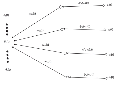
Let the errors generated by $M$ output neurons of the network presented with $N$ training examples be represented in the form of an $N\times M$ matrix.

(1) $E_o=\left[\begin{array}{ccccccc}{e}_1^o\left(1\right)& e_2^o\left(1\right)& e_3^o\left(1\right)& .& .& .& e_M^o\left(1\right)\\ e_1^o\left(2\right)& e_2^o\left(2\right)& e_3^o\left(2\right)& .& .& .& e_M^o\left(2\right)\\ e_1^o\left(3\right)& e_2^o\left(3\right)& e_3^o\left(3\right)& .& .& .& e_M^o\left(3\right)\\ .& .& .& .& .& .& .\\ .& .& .& .& .& .& .\\ .& .& .& .& .& .& .\\ e_1^o\left(N\right)& e_2^o\left(N\right)& e_3^o(N)& .& .& .& e_M^o\left(N\right)\end{array}\right]$(1)

where each row of $E_o$ corresponds to the error generated by the output neurons for a given training pattern.

Similarly, backpropagated errors associated with $Q+1$ hidden neurons of the same network can be represented in the form of an $N\times \left(Q+1\right)$ matrix.

(2) $E_h=\left[\begin{array}{c}{e}_0^h\left(1\right)\\ e_0^h\left(2\right)\\ e_0^h\left(3\right)\\ .\\ .\\ .\\ e_0^h\left(N\right)\end{array}\begin{array}{c}{e}_1^h\left(1\right)\\ e_1^h\left(2\right)\\ e_1^h\left(3\right)\\ .\\ .\\ .\\ e_1^h\left(N\right)\end{array}\begin{array}{c}{e}_2^h\left(1\right)\\ e_2^h\left(2\right)\\ e_2^h\left(3\right)\\ .\\ .\\ .\\ e_2^h\left(N\right)\end{array}\begin{array}{c}.\\ .\\ .\\ .\\ .\\ .\\ .\end{array}\begin{array}{c}.\\ .\\ .\\ .\\ .\\ .\\ .\end{array}\begin{array}{c}.\\ .\\ .\\ .\\ .\\ .\\ .\end{array}\begin{array}{c}{e}_M^h\left(1\right)\\ e_M^h\left(2\right)\\ e_M^h\left(3\right)\\ .\\ .\\ .\\ e_M^h\left(N\right)\end{array}\right]$(2)

The correlation matrix can be evaluated as:

(3) $C_{oh}\left[k,i\right]=\sum _{t=1}^N{e}_k^o\left(t\right)e_i^h\left(t\right)$(3)

where $C_{oh}\left[k,i\right]$ is the entry in the correlation matrix corresponding to the scalar product of the kth column of $E_o$ with the ith column of $E_h$.

Let us examine $C_{oh}\left[3,2\right]$ and $C_{oh}\left[2,2\right]$for the network shown in Figure 1.

Let us assume $C_{oh}\left[3,2\right]>C_{oh}\left[2,1\right]$. According to the MAXCORE principle, $w_{32}$ is more relevant than $w_{21}$ if $\sum _{t=1}^N{e}_3^o\left(t\right)e_2^h\left(t\right)>\sum _{t=1}^N{e}_2^o\left(t\right)e_1^h\left(t\right)$,

where

(4) $e_2^h\left(t\right)=\sum _{k=1}^4{\delta }_k\left(t\right)w_{k2}\left(t\right)$(4)

and

(5) $e_1^h\left(t\right)=\sum _{k=1}^4{\delta }_k\left(t\right)w_{k1}\left(t\right)$(5)

As evident from above equations, higher or lower values of $e_i^h\left(t\right)$ depend not only upon $w_{k1}$ but also upon local gradients ${\delta }_k$of the output neurons connected to the hidden layer neuron i. Since, local gradient of the output neuron k is given by:

(6) ${\delta }_k\left(t\right)=e_k^o\left(t\right){\phi }^{\prime }\left(v_k\left(t\right)\right)$(6)

where $v_k\left(t\right)$ is the induced local field and ${\phi }^{\prime }$ is the differential of the activation function. Most of the time, a sigmoidal activation function is chosen which maps the synaptic weights $w_{ki}\left(t\right)$ nonlinearly in the form of induced local field passed through ${\phi }^{\prime }\left(.\right)$. Since, the contribution of $e_i^h\left(t\right)$ in the magnitude of correlation coefficient $C_{oh}\left[k,i\right]$ depends upon ${\delta }_k\left(t\right)$, which in turn are nonlinear functions of synaptic weights, $w_{ki}\left(t\right)$, a high value of $C_{oh}\left[k,i\right]$ neither guarantees a high magnitude nor a high degree of relevance for $w_{ki}\left(t\right).$ Furthermore, it is always better to define “relevance” of a synaptic weight either in a statistical sense or with respect to a performance metric. The standard practice of complexity regularization defines a risk function as:

(7) $R\left(w\right)={\xi }_s\left(w\right)+\lambda {\xi }_c\left(w\right)$(7)

where ${\xi }_s\left(w\right)$is the standard performance measure (e.g. MSE), and ${\xi }_c\left(w\right)$ is the complexity penalty term which depends upon the network model alone. As regularization parameter, $\lambda$ represents the relative importance of the complexity penalty term with respect to the MSE. Assuming $\lambda$ to have a moderate value somewhere between zero and infinity, the relative importance of complexity penalty term with respect to MSE is also moderate. Therefore, we can define “relevance” of individual synaptic weights both in terms of MSE and in terms of complexity penalty. However, to compute the relevance of weights in terms of ${\xi }_s\left(w\right)$, we need to run BP algorithm first (at least forward pass). For the networks which have not yet undergone training, it would be better to first compute ${\xi }_c\left(w\right)$ in terms of complexity penalty. In the light of the above discussion, novel contributions of this work can be enlisted as follows:

• This work seeks to define relevance of the weights in a statistical sense.

• A coefficient of dominance has been proposed to identify nodes carrying higher information content and to determine complexity penalty for each weight.

• Use of GA to optimize fittest weights in terms of MSE.

• New schemes for initialization of population and mutation have been proposed.

Problem Formulation

The Proposed Methodology

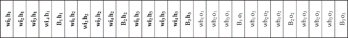
The proposed methodology has been implemented in a sequence of several steps as illustrated in Figure 2. As an illustration of the first stage of the methodology, let us consider an ANN with single hidden layer and three target classes subjected to IRIS data as input. The number of hidden layer neurons has been chosen to be three. As shown in Figure 3, there are a total of 27 connections including 20 weights and 7 biases. All the connections have been initialized randomly. The connections would be evaluated as a part of weight pruning/modification scheme which is described in detail with analytical justifications in the next section. All the 27 connections have been encoded in the form of a chromosome string shown in Figure 4. Many such chromosomes have been generated to initialize the mating pool. Each weight has been encoded using 10 bits. With this step, GA optimization of ANN weights commences. Subsequent steps follow the standard GA flow with crossover, mutation, and ranking of individuals which ultimately yields the “fittest” set of weights. The details of all individual stages of the methodology are described in the implementation section.

Figure 2. The proposed methodology.

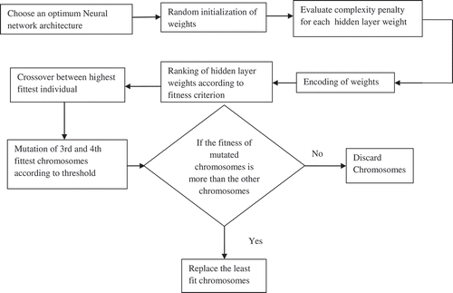
Figure 3. ANN architecture for IRIS data.

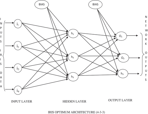
Figure 4. Weights and biases of Figure 2 represented as a chromosome.

Data Description

The simulations have been carried out on several benchmark data sets obtained from UCI machine learning repository. All the data sets chosen for this study represent pattern classification problems with varying number of samples, input dimensions, and target classes details of which is shown in Table 1. During the course of simulation, the number of training and test samples was kept equal in most of the cases except in the case of letter recognition where the results varied significantly when the number of test samples was changed.

Table 1. Data description.

Data set	No. of input dimension	No. of training samples	No. of test samples	No. of classes
IRIS	04	75	75	03
Breast cancer	09	350	349	02
Solar flare	09	500	500	03
Letter rec.1	16	10000	10000	20
Letter rec.2	16	14000	6000	20

Implementation

The Weight Pruning Scheme

The objective of pruning is to downsize the model to the level of least complexity that still provides the best generalization. In general, the capability of feedforward neural networks for data fitting increases as the number of connection weights increase, because an increase in the number of free parameters enables the network to finely capture subtle features. However, a model with too many parameters can pick up nonessential information in the sample data and cause the problem of overfitting. This leads to poor generalization. Therefore, application of appropriate pruning techniques can contribute to improvement in the generalization ability. Furthermore, a reduction in the network components is advantageous for hardware implementation of large-sized ANNs. The proposed idea seeks to incorporate weight pruning scheme into the conventional GA flow. The weights which are insensitive to the error changes can be discarded after each step of training. The pruned network is of smaller size and is likely to give higher accuracy than before its trimming. ANN use network pruning strategies which can be classified into two categories viz. weight decay and weight elimination. In both the strategies, a complexity penalty term is defined which appropriately quantifies the degree of redundancy in a weight. In weight decay procedure, if the initial weight vector is w, the complexity penalty term is defined as the squared norm of the weight vector w (i.e. all the free parameters) in the network and is expressed as:

(8) ${\xi }_c\left(w\right)=w^2={\sum }_{i\in {\zeta }_{total}}{w_i}^2$(8)

where the set ${\zeta }_{total}$ refers to all the synaptic weights in the network. However, in this scheme, some weights in the network have relatively larger values than others. This results in making smaller weights redundant since they have little influence on the training outcome. To overcome this limitation, the complexity penalty term is now redefined as follows:

(9) ${\xi }_c\left(w\right)={\sum }_{i\in {\zeta }_{total}}\left(\frac{{\left(\frac{w_i}{w_o}\right)}^2}{1+{\left(\frac{w_i}{w_o}\right)}^2}\right)$(9)

where w_o is the preassigned weight change parameter defined according to the problem and w_i refers to the ith weight in the network. It is proposed here that the optimality of a weight vector would be defined in the statistical sense. Higher the complexity penalty for a particular weight, more important is the weight for the learning process. If the weights converging on a particular hidden neuron have variance more than the variance of total weights in the network, then that hidden node will contribute more to the network. The real challenge in this case lies in selection of an appropriate $w_o$. As can be inferred from Figure 5, the choice of parameter $w_o$ is crucial aspect of network pruning.

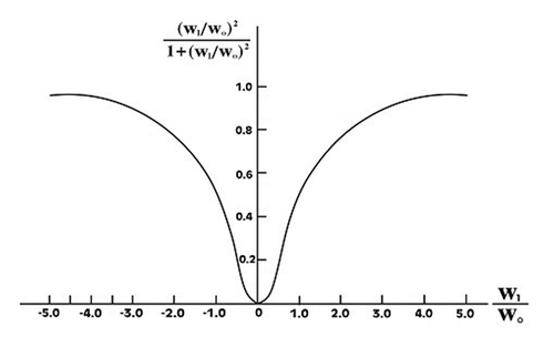
Figure 5. Variation of complexity penalty term with respect to $w_i/w_o$ (Haykin 2007).

In this study, a new pruning method has been proposed based on the weight variation information during the backpropagation training. Every node in the hidden layer is evaluated to determine the effective variance of weights. In order to compute the complexity penalty term as defined in Equation (9) for each weight, a coefficient of dominance called D_si is calculated for each neuron and is expressed as:

(10) $D_{si}=\frac{\overline{V_{total}}}{V_{si}}$(10)

where D_si corresponds to w_o of Equations. (9) and (10), $V_{S_i}$is the variance of the weights of ith hidden node, and ${\bar{V}}_{total}$ is the effective variance of all the weights in the hidden layer.

In the similar way, all the remaining hidden layer neurons are evaluated to find the coefficient of dominance and a set $D$ is defined as:

(11) $D=\left\{D_{S_1},D_{S_2},D_{S_3}\dots \dots \dots D_{S_i}\right\}$(11)

The complexity penalty for each weight in the network is defined as:

(12) ${\xi }_{wi}=\frac{{\left(w_i/D_{S_i}\right)}^2}{1+{\left(w_i/D_{S_i}\right)}^2}$(12)

The variance dependent weight pruning technique described above helps to increase the information content of the weight set convergent on a less dominant neuron. This can be explained in terms of a metric called Fisher information which is defined as a way of measuring the amount of information that an observable random variable X carries about an unknown parameter θ of a distribution that models X and can be stated as:

(13) $\mathrm{\Gamma }\left(\theta \right)=E[{\left(\frac{\mathrm{\partial }ln\left(f\left(X;\theta \right)\right)}{\mathrm{\partial }\theta }\right)}^2|\theta ]$(13)

where log is the natural logarithm of the probability function.

The input to the hidden node is given by:

(14) $y_j=w_{j1}{x}_1+w_{j2}{x}_2+\dots w_{ji}{x}_{\hspace{0.17em}}+b_i$(14)

where $x_i$is the ith input and $w_{ji}$ is the weight from ith input to jth hidden node. Also, the weights leading to a hidden node are regarded as zero mean random variables. Therefore, the mean of the input to the hidden node is given by:

(15) $E\left\{y_j\right\}=E\left\{\sum _{i=0}^n{w}_{ji}{x}_i\right\}=0$(15)

Since, the weights are randomly chosen, they can be considered independent of the input feature. Thus, Equation (9) can be written as:

(16) $E\left\{y_j\right\}=\sum _{i=0}^{n}E\left\{w_{ji}\right\}E\left\{x_i\right\}=0$(16)

The variance of y is given by:

(17) ${\sigma }_y^2=E\left\{{\left(y_j\right)}^2\right\}-E^2\left\{\left(y_j\right)\right\}$(17)

Using Equation (15) in (17), we get,

(18) ${\sigma }_y^2=E\left\{{\left(\sum _{i=0}^n{w}_{ji}{x}_i\right)}^2\right\}$(18)

Since the different weights and input feature to a hidden node are independent, Equation (18) becomes

(19) ${\sigma }_y^2=\sum _{i=0}^{n}E\left\{{\left(w_{ji}\right)}^2\right\}E\left\{{(x_i)}^2\right\}\mathrm{\forall }j$(19)

If the training samples are normalized to be in the interval [0:1], then

(20) $E\left\{{\left(x_i\right)}^2\right\}=E^2\left\{\left(x_i\right)\right\}+{\sigma }_x^2(x_i)$(20)

where ${\sigma }_x^2(x_i)$ is variance of random variable$x_i$. For a uniform random variable lying within [0:1],

(21) $E\left\{{\left(x_i\right)}^2\right\}=\frac{1}{3}$(21)

Also, input to hidden layer weight is also regarded as a random variable with zero mean, uniformly distributed in the interval [–a, a]. Hence, the standard deviation of the input to a hidden layer weight is:

(22) $E\left\{{\left({ }_{ji}\right)}^2\right\}={\frac{a^2}{3}}_{\hspace{0.17em}}$(22)

So, using Equations (13), (15), and (16))

(23) ${\sigma }_y^2=\frac{N{a}^2}{9}$(23)

where N denotes the number of weights converging on a particular node.

Equations (19) and (23) justify that input to a hidden layer neuron is also a random variable with zero mean and $\frac{N{a}^2}{9}$ variance. The probability distribution function of the input to hidden layer node is given as:

(24) $f\left(\mu ,\sigma \right)=\frac{1}{\sqrt{2\pi \sigma }}{e}^{\frac{-{\left(y-\mu \right)}^2}{2{\sigma }^2}}$(24)

where y corresponds to induced local field of jth hidden layer neuron and can also be defined as:

(25) $y_j=\sum _{i=0}^n{w}_{ji}{x}_i$(25)

where x_i is the data input and w_ji is the weight connecting from ith input node to jth hidden node .

According to Equations (23) and (24), the information content about the weight set in the hidden layer neuron which is the above-defined random variable can also be calculated as follows:

(26) $lnf=\mathrm{l}\mathrm{n}\left(\frac{1}{\sqrt{2\pi \sigma }}{e}^{\frac{-{\left(y_j\right)}^2}{2{\sigma }^2}}\right)=ln\frac{1}{\sqrt{2\pi \sigma }}-\frac{y_j^2}{2{\sigma }^2}$(26)

(27) ${\left(\frac{\mathrm{\partial }lnf}{\mathrm{\partial }w}\right)}^2=\frac{y_j^2{x}_i^2}{{\sigma }^4}$(27)

Using Equation (13), the fisher information is given as:

(28) $\mathrm{\Gamma }\left(\theta \right)=E\left[\frac{y_j^2{x}_i^2}{{\sigma }^4}\right]=\frac{1}{{\sigma }^4}E\left[y_j^2\right]E\left[x_i^2\right]$(28)

Using Equations (12), (15), and (17), we get:

(29) $\mathrm{\Gamma }\left(\theta \right)=\frac{N{a}^2}{27{\sigma }^4}$(29)

Let the variance term be replaced by the coefficient of dominance (which is a simple ratio of the variances) and consider two different hidden nodes with $V_{s1}$ and $V_{s2}$ as respective variances of weights convergent on them. Then, the fisher information for the two nodes is given by:

(30) ${\mathrm{\Gamma }}_1\left(\theta \right)=\frac{N{a}^2}{27}{\left(\frac{V_{s1}}{V_{total}}\right)}^4\mathrm{a}\mathrm{n}\mathrm{d}{\mathrm{\Gamma }}_2\left(\theta \right)=\frac{N{a}^2}{27}{\left(\frac{V_{s2}}{V_{total}}\right)}^4$(30)

If $V_{s1}>V_{s2},$ Fisher information of node 1 will be more compared to that of node 2. This implies that a lower coefficient of dominance which makes the complexity penalty higher (and the weight more relevant) also enhances the information content of the convergent connections at a node.

The inclusion of variance in the complexity penalty term and the particular choice of coefficient of dominance are justified by the above explanation.

Genetic Optimization of Weights

Working of Genetic Algorithm

GAs are paradigms for optimization based loosely on several features of biological evolution. Initially, a pool of solutions (population) represented by chromosomes is created. Then, an encoding scheme is used to represent each individual. An evaluation/fitness function is required that provides ranking to each chromosome. The population undergoes reproduction until stopping criteria are met (Sivanandam and Deepa 2007).

The basic GA shown in the form of Figure 6 is explained as follows:

Figure 6. The Genetic Algorithm.

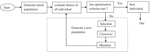
1. Generate random population of chromosomes, that is, suitable solutions for the problem.

2. Fitness of each chromosome in the population is evaluated.

3. The population undergoes reproduction followed by a number of iterations of the following three steps:

   • Parents are selected to reproduce according to their fitness.

   • Different operators are applied to the parents to form new offspring.

   • Place new offspring in the new population.

4. Use new generated population for a further run of the algorithm.

5. If the end criterion is satisfied, return the best solution to the current population.

6. Go to step 2.

Why Genetic Algorithm?

The proposed scheme not only prunes the weights according to the fitness function, it modifies them in accordance with the complexity penalty. The complexity penalty-based modification function yields an initial population of candidates which constitutes the solution space. GA is now used to evaluate the candidate’s fitness through crossover and mutation in successive generations. Actual pruning is accomplished only after the algorithms zeros in on the least fit weights. Weight pruning completely alters the architecture of an ANN. The altered architecture may be better than the original one in terms of convergence and error performance. However, we have no means of judging its optimality before the network is actually trained. From the point of view of custom hardware implementation, repeated alterations in the architecture of a network are highly undesirable and it leads to gross wastage of resources. The use of GA in the subsequent stage ensures efficient search of the solution space to identify one or more “good solutions” though not necessarily the best one. However, through successive generation cycles, it is not hard to identify the least fit (prunable) weight.

The Strategy

The strategy is depicted in the form of a flow chart in Figure 7. As the first step initialization of population is done. Unlike the conventional method of random initialization we adopt a methodology which modifies the initial weights according to the complexity penalty to generate the mating pool in a controlled manner as described below.

Figure 7. Genetic optimization of ANN weights.

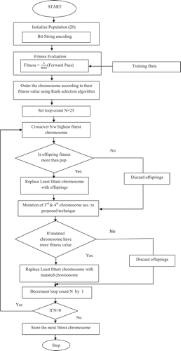
The initialized population of size $K$ is given by a set

(31) $P=\left\{p_i^{\ast j}\right\}j=1,2,3,..K$(31)

Also,

(32) $p_i^{\ast j}=A\ast w_i$(32)

where $A$ is a $1\times K$ vector of multipliers

if ${\xi }_{wi}>0.5$, then $A$ lies in the range [0.9, 1.3].

If $0.2<{\xi }_{wi}\le 0.5$, then $A$ is a $1\times K$ vector of random multipliers.

If $0<{\xi }_{wi}\le 0.2$, then $A$ lies in the range [0.2, 0.5].

If ${\xi }_{wi}<0.2$, then $w_i$ is pruned.

Multiplication of an initial weight $w_i$by $A$ generates $K$ (in our case, $K$ = 20) different weights which constitute the population after bit string encoding. It should be noted that weights with a higher complexity penalty (more relevance) generate a population with “high” complexity penalties (due to range of $A$). Similarly, non-relevant weights generate a population with “low” complexity penalties. By initializing the population in this manner, we are restricting the extremities of the search space to a specified range, thereby reducing the chances of the algorithm running a futile search and getting stuck in local minima. However, the necessity of randomness in initialization cannot be completely overlooked since it is essential to include largest possible number of potential solutions in the search space. To ensure this, we have generated random population from the weights having “moderate” complexity penalty.

The fitness function is defined as $\frac{1}{MSE}$

(33) $\mathrm{w}\mathrm{h}\mathrm{e}\mathrm{r}\mathrm{e},\mathrm{M}\mathrm{S}\mathrm{E}=\frac{1}{2}\sum _{\mathrm{p}=1}^{\mathrm{N}}{\left({\mathrm{t}}^{\mathrm{p}}-{\mathrm{y}}^{\mathrm{p}}\right)}^2$(33)

Here, t and y represent the target and calculated outputs, respectively, and p signifies the number of training patterns. Fitness of each chromosome is evaluated by running the forward pass of BP algorithm. The chromosomes are ordered according to their fitness value using rank selection. Reproduction of new offspring is done by selecting fittest parents from the mating pool and subjecting them to two point restricted crossover.

Each generation cycle witnesses addition of the offspring to the mating pool if its fitness is more than that of one of its parents. In this case, the least fit chromosome is discarded and the offspring is ranked according to its fitness value. However, the offspring is discarded if it is not fitter than any of its parents. In both cases, third and fourth fittest chromosomes are mutated with a small mutation probability (0.06–0.09). If the mutated chromosomes are fitter than the original one, they are added to the mating pool and ranked accordingly and two least fit chromosomes are discarded. This heuristic step of mutating third and fourth rank chromosomes is like giving a “second chance” to some athlete taking part in Olympics and missing the bronze medal by a whisker. If mutation with a small probability increases the fitness then both original and mutated weights should be part of the mating pool in the next generation cycle. After 25 generation cycles, the average increase in fitness of weights was no longer significant employing the proposed scheme. The fitness values of the weights obtained using the proposed technique were compared with that obtained using conventional GA (random initialization) and it was verified that partially random initialization and mutation of third and fourth fitted chromosomes yielded fitter individuals in significantly less number of generation cycles.

Training the Pruned ANN

After 25 generation cycles of the GA, the pruned ANN is reinitialized with the stored weights. A single hidden layer neural network was trained using two different versions of BP algorithm for classifying five benchmark data sets. The number of hidden layer neurons was optimized experimentally and different architectures were found optimum for different data set. The network was first trained using traingdm function of Matlab. traingdm was chosen as the training function because it gives the highest degree of freedom for the investigator to fine tune the training parameters since both learning rate and momentum constant can be varied experimentally using this function. The network was also trained with Levenberg–Marquardt algorithm using trainlm function of MATLAB. Since, Levenberg–Marquardt algorithm is known to outperform simple gradient descent and other conjugate gradient methods in a plentitude of problems, it was necessary to examine whether the proposed technique is able to improve the performance of Levenberg–Marquardt algorithm. A 10-fold cross validation scheme was used to prevent over fitting. The training phase performance of the network in was evaluated with respect to four parameters viz. convergence success rate (% of time the simulation reaches error goal), mean epochs, execution time, and computational complexity. However, the generalization performance is the ultimate performance metric which gives the classification success rate. All the parameters have been evaluated both for unpruned and pruned networks.

Results and Discussions

Convergence and Generalization

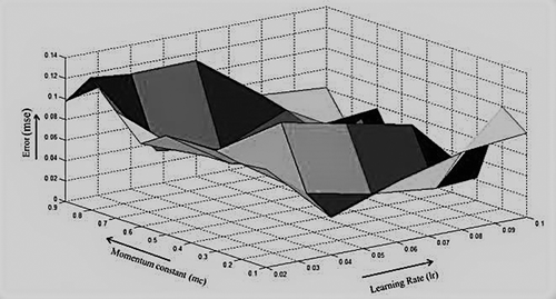
The training phase performances of the conventional ANN and GA-optimized ANN trained with traingdm are given in Tables 2 & 3, respectively. In Table 2, results are shown for the networks not subjected to GA-based weight optimization. It can be observed that the pruned architectures perform marginally better than their unpruned counterparts for all the three training parameters. A comparison of Tables 2 and 3 reveals significant improvements in the performance of the ANN when the weights are optimized using GA. Furthermore, better performance of the pruned architectures can’t be ignored in this case also. The networks were then trained till convergence and subsequently presented with the test samples. Figures 8 and 9 depict the error surface obtained using conventional BP and proposed algorithm, respectively. As evident from the plots, the error surface obtained using the proposed technique spans a larger area of the plot with multiple error minima. This indicates more consistent performance of the network initialized with GA-determined weights at almost all values of learning rate and momentum constant. The effect of the proposed techniques on Levenberg–Marquardt algorithm has been investigated. The pruned networks have again performed marginally but consistently better with trainlm as shown in Table 4. Although trainlm by default exhibits higher converge success and a lower epoch mean, GA-optimized weights have improved these parameters as can be observed in Table 5.

Table 2. Training phase performance of conventional ANN (traingdm).

Data set	Convergence success (%)		Epoch mean		Execution time (sec)
	Unpruned network	Pruned network	Unpruned network	Pruned network	Unpruned network	Pruned network
IRIS	100	100	402.5	400	208	200
Breast cancer	90.5	94.5	1180	1000	410	420
Solar flare	90.2	92.5	1260	1130	542	500
Letter rec.1	75.5	78.5	5805.5	4972.5	360	1200
Letter rec.2	76.6	78	7280	6940	500	2300

Table 3. Training phase performance of GA-optimized ANN (traingdm).

	Convergence success (%)		Epoch mean		Execution time (sec)
Data set	Unpruned network	Pruned/ modified network	Unpruned network	Pruned/ modified network	Unpruned network	Pruned/ modified network
IRIS	100	100	325	300	178	164
Breast cancer	96	100	978	745	240	220
Solar flare	95.6	98	1034.5	940.4	342	300
Letter rec.1	76	96	4220.6	3150	760	600
Letter rec.2	74	95.2	6670	5500	1500	1224

Table 4. Training phase performance of conventional ANN (trainlm).

Data set	Convergence Success (%)		Epoch mean		Execution time (sec)
	Unpruned network	Pruned/modified Network	Unpruned network	Pruned/ modified network	Unpruned network	Pruned/ modified network
IRIS	100	100	56	50	14	13
Breast cancer	100	100	255	200	22	20
Solar flare	98.2	98	388	325.5	28	26
Letter rec.1	80	82	1059.5	1002	66	64
Letter rec.2	78	80.5	1987	1526	110	100

Table 5. Training phase performance of GA-optimized ANN (trainlm).

Data Set	Convergence Success (%)		Epoch Mean		Execution Time (Sec)
	Unpruned Network	Pruned/ Modified Network	Unpruned Network	Pruned/ Modified Network	Unpruned Network	Pruned/ Modified Network
IRIS	100	100	44	30	08	08
Breast Cancer	100	100	126	120	12	11
Solar Flare	98.2	100	200	176	18	15
Letter Rec.1	85	92	598	500	24	22
Letter Rec.2	82	86	1020	918	40	34

Figure 8. Surface plot for error obtained for the network trained using conventional backpropagation.

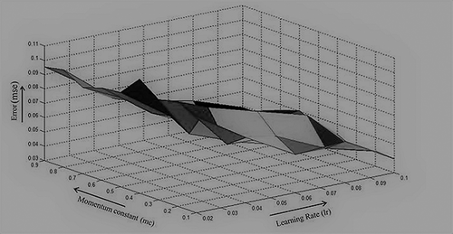
Figure 9. Surface plot for error obtained for the network trained using GA-optimized backpropagation.

The reflection of better convergence in the training phase on the generalization performance was as expected and the results are shown in Tables 6 and 7 for traingdm and in Tables 8 and 9 for trainlm, respectively. It is encouraging to note that magnitude of improvement in the performance matrices is more significant in complicated architectures e.g. “letter recognition-1 and 2”. Intuitively, more complex architectures have larger number of weights and hence more candidates in the mating pool leading to the fittest possible selection.

Table 6. Generalization performance of conventional ANN (traingdm).

		No. of correctly classified samples/success rate (%)
Data set	Total no. of test samples	Unpruned network	Pruned network
IRIS	75	66/88	66/88
Breast cancer	349	158/45.27	188/53.87
Solar flare	500	195/39	227/45.40
Letter rec.1	10,000	4254/42.54	5502/55.02
Letter rec.2	6000	2642/44.03	2972/49.53

Table 7. Generalization performance of GA Optimized ANN (traingdm).

Data set	Total no. of test samples	No. of correctly classified samples/success rate (%)
		Unpruned network	Pruned network
IRIS	75	69/92	70/93.33
Breast cancer	349	208/59.59	240/68.76
Solar flare	500	242/48.40	307/61.40
Letter rec.1	10,000	5200/52	5772/57.72
Letter rec.2	6000	2986/49.76	3655/60.91

Table 8. Generalization performance of conventional ANN (trainlm).

Data set	Total no. of test samples	No. of correctly classified samples/success rate (%)
		Unpruned network	Pruned network
IRIS	75	70/93.33	70/93.33
Breast cancer	349	258/73.92	278/79.65
Solar flare	500	295/59	320/64
Letter rec.1	10,000	5270/52.70	6208/62.08
Letter rec.2	6000	3642/60.70	4006/66.76

Table 9. Generalization performance of GA-optimized ANN (trainlm).

Data set	Total no. of test samples	No. of Correctly Classified Samples/Success Rate (%)
		Unpruned network	Pruned network
IRIS	75	72/96	72/96
Breast cancer	349	290/83.1	302/86.53
Solar flare	500	308/61.60	351/70.20
Letter rec.1	10,000	5690/56.90	6502/65.02
Letter rec.2	6000	4006/66.76	4105/68.41

Computational Cost

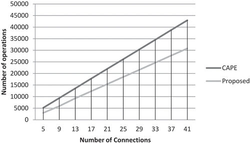
The computational cost (complexity) is an important issue to be addressed during evaluation of algorithms. Sometimes, the algorithm’s effectiveness in providing a solution to a given problem requires the execution of complex computations and the use of excessive memory resources, which can create severe difficulties in real-time or low-cost applications. Let us analyze first the computational complexity of the weight pruning stage described in section “The weight pruning scheme.” Since we have developed the weight pruning scheme as an alternative to CAPE, we would now compare the computational cost for these two methodologies. Tables 10 and 11 enlist the number of operations required by the proposed scheme and CAPE, respectively, as a function of number of input samples (N), input attributes (P), hidden neurons (Q), and output neurons (M). The number of operations required by the proposed methodology and CAPE was computed considering an MLP with N = 140 input samples, P = 2 input attributes, M = 1 output neuron, and the number of hidden neurons Q varying from 1 to 10. The same MLP was taken as reference by the inventors of CAPE (Medeiros and Barreto 2013).

Table 10. Computational operations required by the proposed method.

Operation	Number of operations as a function of N, P, M, Q
Addition	N(3PQ+ 3Q+ M)
Subtraction	N(3PQ+ 3Q+ M)
Multiplication	N(2PQ+ 2Q+ M)
Division	N(PQ+ 2Q)
Tanh	-

Table 11. Computational operations required by CAPE method (Medeiros and Barreto 2013).

Operation	Number of operations as a function of N, P, M, Q
Addition	N(3PQ+ 3QM-P + 2Q+ 3M-2)-PQ-QM-M-1
Subtraction	N(Q + 2M)
Multiplication	N(4PQ+ 4QM+ 5Q+ 5M)
Division	-
Tanh	N(Q + M)

It can be easily observed from the tables that the proposed scheme requires lesser number of multiplication operations than CAPE. This is due to the fact that CAPE requires calculation of correlation coefficients to determine the relevance of weights, whereas we define relevance in terms of complexity penalty which involves fewer operations. Furthermore, unlike the proposed technique, CAPE involves running backward pass of BP which in turn involves computations through a nonlinear activation function incurring additional cost as shown in the last row of the tables. Figure 10 shows how the number of operations varies as a function of number of weights (connections). For the sake of simplicity, all the operations are considered to have same computational cost. From the graph, it is apparent that the proposed scheme demands lesser resources than the CAPE algorithm. It is also clear from Table 12 that using proposed weight pruning stage, there is substantial reduction in the computational complexity and this reduction tends to become consistent with increasing number of connections.

Table 12. Percentage reduction in complexity by the proposed algorithm.

No. of connections	% Age reduction in complexity (w.r.t. CAPE)
5	42.41545894
9	37.25992318
13	31.9036038
17	30.65405831
21	29.8820744
25	29.35779817
29	28.97848931
33	28.69132373
37	28.46636216
41	28.28536835

Figure 10. Estimated costs for CAPE and proposed scheme when pruning an MLP.

Table 13 presents the stage-wise breakup of computations up to the commencement of GA. As we know, the computational complexity of GA is of the order $O\left(G\ast n\ast b\right)$, Where $G$, $n$, and $b$ are number of generations, population size, and bit string length, respectively. In our case, this stage gives a complexity of $O\left(25\ast 20\ast 10\right)$. In addition to it, evaluation of fitness for each weight requires running of forward pass of BP once per generation cycle which requires $O\left(\frac{P\ast M\ast N\ast G}{2}\right)$ operations. BP without GA requires $O\left(P\ast M\ast N\ast E\right)$ operations, where $E$ is the number of epochs. This means savings in terms of mean epochs is going to decide which technique consumes lesser number of operations. It is evident from Tables 2–5, $E>\frac{G}{2}$ for most of the architectures and even for Levenberg–Marquardt algorithm which takes much fewer epochs to converge.

Table 13. Stage wise break-up of computations.

S.No.	Stage	Operations	Computations
1.	Mean of hidden layer weights	Addition	N(P + 1)Q
2.	Variance of hidden layer weights	Subtraction multiplication	N(P + 1)Q N(P + 1)Q
3.	Coefficient of dominance	Addition division	N(P + 1)Q NQ
4.	Complexity penalty	Division multiplication addition	N(P + 1)Q N(P + 1)Q N(P + 1)Q
5.	Threshold multiplication	Multiplication	N(P + 1)Q

Example: Pruned Network A: Trained with conventional trainlm (IRIS data). Epoch mean = 50.

Pruned Network B: Trained with GA optimized trainlm (IRIS data). Epoch mean = 30.

   Computational complexity of network A        = $O\left(P\ast M\ast N\ast E\right)$ = O $\left(4\ast 3\ast 150\ast 50\right)$ = $O\left(90,000\right)$

   Computational complexity of network B              = $O\left(\frac{4\ast 3\ast 150\ast 25}{2}\right)+O\left(4\ast 3\ast 150\ast 30\right)+O\left(25\ast 20\ast 10\right)$ $=O\left(81,500\right)$.

Thus, the savings in computations even for marginal improvement in epoch mean due to GA optimization is evident and this has been observed more prominently in complex architectures which take large number of epochs to converge.

Conclusion

The results presented in the previous section confirm the efficacy of the proposed technique in terms of convergence, execution time, and generalization performance. It is evident that both weight pruning and GA optimization stages play their respective parts and contribute significantly to improvement in performance of the BP-trained ANN. This improvement is reflected not only in ANN trained with traditional gradient descent with momentum term (traingdm) but also with a more advanced algorithm like Levenberg–Marquardt (trainlm). Reduction in the epochs required for convergence indicates that GA search about the weight space has yielded near optimal solutions. Initialization of population based upon complexity penalty as described in section “Implementation” seems to have paid dividend. Subsequently, the mutation of third- and fourth-ranked individuals (described as MAD algorithm) in the mating pool makes the whole process more competitive since the mutation operator seeks to increase the appropriateness of the weights in a statistical sense. Evaluation with the MSE-based fitness function also points toward a correlation between statistical “relevance” of weights and their fitness in terms of lower MSE. The computational complexity of the proposed weight pruning stage has been proven to be better than the existing weight pruning strategy CAPE. Also, the classification results obtained reveal the efficacy of the proposed technique. It can also be concluded that this approach can serve as an efficient and viable alternative to conventional neuro-genetic design of neural classifiers. Future work may be in the direction of further reducing the execution time of the proposed algorithm.

Disclosure Statement

The authors report no conflicts of interest. The authors alone are responsible for the content and writing of the paper. The Manuscript has not been published elsewhere and it has not been submitted simultaneously for publication elsewhere.

Additional information

Funding

This research did not receive any specific grant from funding agencies in the public, commercial, or not-for-profit sectors.

References

- Aleksander, I., and J. Taylor. 1992. Pruning neural nets by genetic algorithm. Artificial neural networks 2. International Conference on Artificial Neural Networks (ICANN-92). Brighton, United Kingdom: Elsevier Science Publishers.
- Asmaa, A. N., A. T. Erdogan, and T. Arslan. 2013. Adaptive three-dimensional cellular genetic algorithm for balancing exploration and exploitation processes. Soft Computing 17:1145–57. doi:10.1007/s00500-013-0990-1.
- Augasta, M. G., and T. Kathirvalavakumar. 2015. Pruning algorithms of neural networks – a comparative study. Central European Journal of Computer Science 3 (3):105–15.
- Bull, L. 2001. On Co-evolutionary genetic algorithms. Soft Computing 5:201–07. doi:10.1007/s005000100082.
- Christiansen, N., J. Job, K. Klyver, and J. Hogsberg. 2012. Optimal brain surgeon on artificial neural networks in nonlinear structural dynamics. 25th Nordic seminar on computational mechanics. Lund, Sweden.
- Haupt, S. E., and R. L. Haupt. 2011. A mixed integer genetic algorithm used in biological and chemical defense applications. Soft Computation 15 (1):51–59. doi:10.1007/s00500-009-0516-z.
- Haykin, S. 2007. Neural network and learning machines. India: Prentice-HALL.
- Hu, L., L. Qin, K. Mao, and W. Chen. 2015. Optimization of neural network by genetic algorithm for flowrate determination in multipath ultrasonic gas flowmeter. IEEE Sensors Journal 16 (5):1158–67. doi:10.1109/JSEN.2015.2501427.
- Hunter, A., and K. S. Chiu. 2000. Genetic algorithm design of neural network and fuzzy logic controllers. Soft Computation 4:186–92. doi:10.1007/s005000000050.
- Karlra, P., and N. R. Prakash. 2003. A neuro-genetic algorithm approach for solving the inverse kinematics of robotic manipulators. IEEE Conference on Systems, Man and Cybernetics 2. Washington, USA: IEEE Publishers.
- Karthikeyan, P., S. Baskar, and A. Alphones. 2012. Improved genetic algorithm using different genetic operator combinations (GOCs) for multicast routing in ad hoc networks. Soft Computing 17 (9):1563–72. doi:10.1007/s00500-012-0976-4.
- Kingston, G., H. Maier, and M. Lambert. 2004. A statistical input pruning method for artificial neural networks used in environmental modeling. Biennial Meeting of the International Environmental Modelling and Software Society. Osnabruck, Germany: iEMSs Publisher.
- Kumar, P., D. Gospodaric, and P. Bauer. 2007. Improved genetic algorithm inspired by biological evolution. Soft Computation 11 (10):923–41. doi:10.1007/s00500-006-0143-x.
- Kwon, Y. K., and B. R. Moon. 2007. A hybrid neurogenetic approach for stock forecasting. IEEE Trans. Neural Network 18 (3):851–64. doi:10.1109/TNN.2007.891629.
- Libelli, S., Marsili, and P. Alba. 2000. Adaptive mutation in genetic algorithms. Soft Computation 4 (2):76–80. doi:10.1007/s005000000042.
- Lin, C. T., M. Prasad, and A. Saxena. 2015. An improved polynomial neural network classifier using real-coded genetic algorithm. IEEE transactions on systems. Man, and Cybernetics: Systems 45 (11):1389–401.
- Ling, S. H., and F. H. F. Leung. 2007a. An improved genetic algorithm with average-bound cross over and wavelet mutation operations. Soft Computation 11 (1):7–31. doi:10.1007/s00500-006-0049-7.
- Ling, S. H., F. H. F. Leung, and H. K. Lam. 2007b. Input-dependent neural network trained by real-coded genetic algorithm and its industrial applications. Soft Computation 11 (11):1033–52. doi:10.1007/s00500-007-0151-5.
- Louis, S. J. 2005. Genetic learning for combinational logic design. Soft Computation 9 (1):38–43. doi:10.1007/s00500-003-0332-9.
- Mantzaris, D., G. Anastassopoulos, and A. Adamopoulos. 2011. Genetic algorithm pruning of probabilistic neural networks in medical disease estimation. Neural Networks 24 (8):831–35. doi:10.1016/j.neunet.2011.06.003.
- Medeiros, C. M., and G. A. Barreto. 2013. A novel weight pruning method for MLP classifiers based on the MAXCORE principle. Neural Computing and Applications 22 (1):71–84. doi:10.1007/s00521-011-0748-6.
- Mesquita, D. P., J. Gomes, R. L. Rodrigues, and R. K. Galvao. 2015. Pruning extreme learning machines using the successive projections algorithm. IEEE Latin America Transactions 13 (12):3974–79. doi:10.1109/TLA.2015.7404935.
- Ramasubramanian, P., and A. Kannan. 2006. A genetic-algorithm based neural network short-term forecasting framework for database intrusion prediction system. Soft Computation 10 (8):699–714. doi:10.1007/s00500-005-0513-9.
- Reed, R. 1993. Pruning algorithms-A survey. IEEE Transactions on Neural Networks 4 (5):740–47. doi:10.1109/72.248452.
- Sabo, D., and X. Yu. 2008. A new pruning algorithm for neural network dimension analysis. IEEE World Congress on computational Intelligence Proc. Hong Kong, China.
- Samanta, B., K. R. Al-Balushi, and S. A. Al-Araimi. 2006. Artificial neural networks and genetic algorithm for bearing fault detection. Soft Computation 10 (3):264–71. doi:10.1007/s00500-005-0481-0.
- Sivanandam, S. N., and S. N. Deepa. 2007. Introduction to Genetic Algorithms. Berlin, Heidelberg: Springer Science & Business Media.
- Srivastava, A. K., K. K. Shukla, and S. K. Srivastava. 1998. Exploring neuro-genetic processing of electronic-noise data. Microelectronics Journal 29 (11):921–31. doi:10.1016/S0026-2692(98)00056-1.
- Tan, F., X. Fu, Y. Zhang, and A. G. Bourgeois. 2008. A genetic algorithm-based method for feature subset selection. Soft Computation 12 (2):111–20. doi:10.1007/s00500-007-0193-8.
- Tong, Z., and G. Tanaka. 2015. A pruning method based on weight variation information for feedforward neural networks. 4th IFAC Conference on Analysis and Control of Chaotic Systems 48(18): 221–226. Elsevier Science Publishers
- UCI machice learning repository http://archive.ics.uci.edu/ml/datasets
- Yang, S. H., and Y. P. Chen. 2012. An evolutionary constructive and pruning algorithm for artificial neural networks and its prediction applications. Neurocomputing 86 (1):140–49. doi:10.1016/j.neucom.2012.01.024.