Variable Selection for Artificial Neural Networks with Applications for Stock Price Prediction

ABSTRACT

We propose a new Artificial neural network (ANN) method where we select a set of variables as input variables to the ANN. The selection is made so that the input variables may be informative for a target variable as much as possible. The proposed method compared favorably with the existing ANN methods when their performances were evaluated based on 488 stocks in S&P500 in terms of prediction accuracy.

Introduction

Stock price predictions have been made based on a group of statistical models that are suitable for representing the stock price data. Those models are given as variations of the autoregressive moving average model (ARMA) (Whittle 1951) where the current stock price is expressed as a linear combination of some past prices and errors. One of the most popular variations is the autoregressive integrated moving average model (ARIMA) (Box and Jenkins 1976) where one can consider price differences as terms in the model. Although we may expand the model to a polynomial type of model, nonlinearity of the model is quite limited.

This limitation is well addressed by using neural network methods. Artificial neural networks (ANNs) have been applied with a good level of performance (Kar 1990; Zekic 1998; Pakdaman, Taremian and Hashmi 2010). According to Cybenko (Cybenko 1989) and Hornik (Hornik 1991), any nonlinear relationship among the data can be modeled by ANNs without distributional assumptions. The ANN is usually constructed by applying the back-propagation of errors (Rumelhart, Hinton, and Williams 1986; Werbos 1990).

One of the drawbacks of ANN is overfitting, which means that the ANN tends to be too good to data to use it for prediction. A remedy for this is making the ANN simpler by controlling the number of input variables rather than using all the possible variables in the input basket. Research in this line is not rare (Blum and Langley 1997; Guyon and Elisseeff 2003; Kohavi and John 1997; May, Dandy, and Maier 2011). For example, Grigoryan (Grigoryan 2015) used the principle components analysis (PCA) result for building an ANN with improved prediction accuracy.

In this paper, we propose a method for improving the prediction accuracy with ANNs by selecting the input variables which are informative for the target variable. By this approach, we could possibly obviate overfitting and keep the level of complexity of ANN as low as possible.

The paper is organized as follows. In second section, we will describe briefly our models to use as a preliminary. We will then describe the procedure of our method in third section using a set of the stock price data of Apple Inc.. Performance comparison is made in fourth section among the methods for ANNs using the stock price data of the S&P500 companies. Finally, in fifth section, we discuss the implication of the results with a summary.

Preliminaries

ANNs are supervised learning tools for classification and regression. A multi-layer perceptron (MLP) is an ANN structure which consists of at least three layers of neurons: an input layer, a number of hidden layers, and an output layer. It is a feedforward neural network where each adjacent pair of layers is a directed and weighted bipartite graph. Figure 1 displays a simple MLP structure for regression which has a single hidden layer.

Figure 1. A simple MLP architecture.

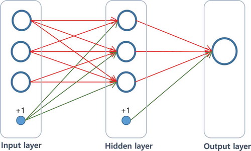
Figure 2. The IAMB algorithm for Markov blanket discovery (Tsamardinos, Aliferis, and Statnikov 2003).

Let $L$ be the number of layers, $n_i$ be the number of neurons or nodes in the $i$th layer for $i=1,\cdots ,L$. Assume that the input layer is of $n_1$ neurons and denote the input data by $x=\left\{x_1,\cdots ,x_{n_1}\right\}$. Then the activations of neurons in the input layer are set to be $a_1^{(1)}(x)=x_1,\cdots ,a_{n_1}^{(1)}(x)=x_{n_1}$. The activation of the $j$th neuron in the $i$th layer $a_j^{(i)}(x)$ ($i=2,\cdots ,L$) is defined by

(1) $a_j^{(i)}(x)=f\left(\sum _{k=1}^{n_{i-1}}{w}_{kj}^{(i-1)}{a}_k^{(i-1)}(x)+b_j^{(i-1)}\right)$(1)

where $w_{kj}^{(i-1)}$ is the edge weight on the edge connecting the $k$th neuron in the $(i-1)$th layer and the $j$th neuron in the $i$th layer and $b_j^{(i-1)}$ represents the intercept term at the $(i-1)$th layer for the $j$th neuron in the $i$th layer. The function $f$ is a nonlinear function called an activation function. A common choice is a logistic function $f(x)=\frac{1}{1+e^{-x}}$ or a hyperbolic tangent function $f(x)=\frac{e^x-e^{-x}}{e^x+e^{-x}}$. The output of a MLP is obtained as the weighted linear sum of the activations of the hidden neurons.

If we want to construct an ANN model for time series data, the model can be expressed as a nonlinear function with an error such as

$y_t=F(y_{t-1},y_{t-2},\cdots ,y_{t-d_y})+{ϵ}_t$

where $F$ is a nonlinear function, $d_y$ a time order of $y$, and ${\epsilon }_t$ a noise at time $t$. If, in addition, there are exogenous inputs $\left\{u_t\right\}$ to the data, the model is expressed as:

(2) $y_t=F(y_{t-1},y_{t-2},\cdots ,y_{t-d_y},u_{t-1},u_{t-2},\cdots ,u_{t-d_u})+{ϵ}_t$(2)

where $d_u$ is the time order of $u$. This model is called a nonlinear autoregressive exogenous model (NARX). If this model is substantiated as an ANN, its input layer is of $d_y+d_u+1$ neurons.

Since it is desirable that we avoid overfitting while making predictions as accurate as possible, we aim to construct an ANN where the input variables are selected based on data which are mostly informative for the target variable. The input variables may not be related linearly with the target variable. So the variable selection approach for statistical linear regression analysis may not work properly. We will rather use, for the variable selection, a score function such as the mutual information measure between variables conditional on some other variables. This approach is well accepted for learning Bayesian networks. One of the algorithms well known for this learning is the Incremental Association Markov Blanket (IAMB) algorithm (Tsamardinos, Aliferis, and Statnikov 2003). This algorithm searches for the smallest set of random variables given which a variable of interest is conditionally independent of the remaining random variables in a Bayesian network model. The smallest set is called a Markov blanket. We will use this algorithm in search of a Markov blanket of the target variable and use the Markov blanket for the input layer of an ANN. This variable selection process is described in detail in next section.

Methodology

Data Collection and Pre-Processing

The daily stock prices of 488 companies in S&P500 are collected from the website of yahoo finance, for the period of May 30, 2012–March 31, 2017, where the total number of time points is 1218 for each company. The five daily components of the stock price are Open, High, Low, Close, and Volume which are explained in Table 1.

Table 1. The daily components of the stock price.

Components	Description
Open	An opening price
High	A highest price for a day
Low	A lowest price for a day
Close	A closing price
Volume	Traded volume for a day

We assume a NARX model given by:

(3) $y_{t+1}=F(y_t,y_{t-1},\cdots ,y_{t-7},u_t)+{ϵ}_{t+1},$(3)

where $\left\{y_t\right\}$ is the time series of closing stock prices. The value $d_y$ in Equation (2) is set at 7 and $d_u$ at 1, meaning that we use only the current exogenous variables $u_t$. $u_t$ is a four-dimensional vector as:

(4) $u_t=\left\{Ope{n}_t,Hig{h}_t,Lo{w}_t,Volum{e}_t\right\}.$(4)

Model (3) can then be written as:

(5) $\begin{array}{c}Clos{e}_{t+1}=F(Clos{e}_t,Clos{e}_{t-1},\cdots ,Clos{e}_{t-7},Ope{n}_t,Hig{h}_t,\\ Lo{w}_t,Volum{e}_t)+{ϵ}_{t+1}\end{array}$(5)

The data available for Equation (5) is of 1211 time points, where the first and last few observations for Apple Inc. are in Table 2.

Table 2. Stock price data of Apple Inc.

Date	$Ope{n}_t$	$Hig{h}_t$	$Lo{w}_t$	$Volum{e}_t$	$Clos{e}_{t+1}$	$Clos{e}_t$	$Clos{e}_{t-1}$	$\cdots$	$Clos{e}_{t-7}$
12.06.08	81.7	82.9	81.3	86879100	81.6	82.9	81.7	$\cdots$	82.7
12.06.11	84.0	84.1	81.5	146816200	82.3	81.6	82.9	$\cdots$	82.5
$⋮$	$⋮$	$⋮$	$⋮$	$⋮$	$⋮$	$⋮$	$⋮$	$\ddots$	$⋮$
17.03.30	144.2	144.5	143.5	21207300	143.7	143.9	144.1	$\cdots$	139.8
17.03.31	143.7	144.3	143.0	19661700	143.7	143.7	143.9	$\cdots$	141.4

The variable $Clos{e}_{t+1}$ represents the closing stock price of the next day to predict. The data are divided into two parts; 80% of the data (969 data points) are chosen randomly for the training set to build a model and the remaining 20% (242 data points) for the test set.

Learning Bayesian Network Structure

Let $\mathfrak{X}=\left\{X_1,\cdots ,X_p\right\}$ be a set of the random variables involved in a model. Then, the Markov blanket of a random variable $X_i$ is defined as a minimal set $S$ of random variables such that when it is conditioned, $X_i$ is independent of the rest of random variables $\left\{X_1,\cdots ,X_p\right\}\mathrm{\setminus }S$. The Markov blanket is identified as the union of the set of parent nodes of node $i$, the set of child nodes $i$, and the spouse nodes of $i$ in the Bayesian network structure.

There are many algorithms for learning Bayesian networks from data. In this work, we used the IAMB algorithm to construct a Bayesian network structure for the 13 variables in Equation (5). For our model, the set $\mathfrak{X}$ is

(6) $\begin{array}{c}\left\{Clos{e}_{t+1},Clos{e}_t,Clos{e}_{t-1},\cdots ,Clos{e}_{t-7},Ope{n}_t,Hig{h}_t,Lo{w}_t,Volum{e}_t\right\}.\end{array}$(6)

The IAMB algorithm finds the Markov blanket for each variable $T\in \mathfrak{X}$ by the procedure in Figure 2.

1. Set the current Markov blanket $CMB=\mathrm{\varnothing }$.

2. While $CMB$ has changed, find the variable $X$ in $\mathfrak{X}-CMB-\left\{T\right\}$ that maximizes $I(X,T|CMB)$. If $X$ and $T$ are not independent given $CMB$, then add $X$ to $CMB$.

3. Remove form $CMB$ all variables $X$, for which $X$ and $T$ are independent given $CMB-\left\{X\right\}$.

4. Set $CMB$ as a Markov blanket of $T$, denoted by $MB(T)$.

It is common to use the Kullback–Leibler divergence measure as a measure of conditional independence of $X$ and $Y$ given $Z$ that is defined as:

(7) $I(X,Y|Z)={\int }_Z{\int }_Y{\int }_{X}p(x,y,z)log\frac{p(x,y,z)p(z)}{p(x,z)p(y,z)}dxdydz.$(7)

Under the Gaussian assumption on $(X,Y,Z)$, we can easily find (Gel’fand and Yaglom 1957) that:

(8) $I(X,Y|Z)=-\frac{1}{2}log(1-{\rho }_{XY|Z}^2).$(8)

where ${\rho }_{XY|Z}$ is the partial correlation of $X$ and $Y$ given $Z$. The partial correlation ${\rho }_{XY|Z}$ can be estimated by the sample partial correlation using the training set of data. The sample partial correlation ${\hat{\rho }}_{XY|Z}$ can be computed by:

(9) ${\hat{\rho }}_{XY|Z}=\frac{{\hat{\rho }}_{XY}-{\hat{\rho }}_{XZ}{\hat{\rho }}_{YZ}}{\sqrt{1-{\hat{\rho }}_{XZ}^2}\sqrt{1-{\hat{\rho }}_{YZ}^2}}$(9)

where ${\hat{\rho }}_{XY}$, ${\hat{\rho }}_{XZ}$, and ${\hat{\rho }}_{YZ}$ are the sample correlations. For example, with the training set of size 969, we can calculate the sample correlation of $Clos{e}_t$ and $Hig{h}_t$ by the formula:

(10) ${\hat{\rho }}_{Clos{e}_t,Hig{h}_t}=\frac{\sum _{i=1}^{969}(Clos{e}_t^{(i)}-Cl\bar{o}se)(Hig{h}_t^{(i)}-H\bar{i}gh)}{\sqrt{\sum _{i=1}^{969}{(Clos{e}_t^{(i)}-Cl\bar{o}se)}^2}\sqrt{\sum _{i=1}^{969}{(Hig{h}_t^{(i)}-H\bar{i}gh)}^2}}$(10)

where $\bar{X}$ is the average of the $X_t$’s.

If the size of a conditioning set is larger than one, then ${\hat{\rho }}_{XY|Z}$ can be computed by the following recursive formula. For any $Z_0\in Z$,

(11) ${\hat{\rho }}_{XY|Z}=\frac{{\hat{\rho }}_{XY|Z\mathrm{\setminus }\left\{Z_0\right\}}-{\hat{\rho }}_{X{Z}_0|Z\mathrm{\setminus }\left\{Z_0\right\}}{\hat{\rho }}_{Y{Z}_0|Z\mathrm{\setminus }\left\{Z_0\right\}}}{\sqrt{1-{\hat{\rho }}_{X{Z}_0|Z\mathrm{\setminus }\left\{Z_0\right\}}^2}\sqrt{1-{\hat{\rho }}_{Y{Z}_0|Z\mathrm{\setminus }\left\{Z_0\right\}}^2}}.$(11)

Also, the test of the conditional independence of $X$ and $Y$ given $Z$ is based on the $t$-test, which is implemented with the statistic

(12) $T=\sqrt{n-2-\left|Z\right|}\frac{{\hat{\rho }}_{XY|Z}}{\sqrt{1-{\hat{\rho }}_{XY|Z}^2}},$(12)

where $n=969$, the size of the training set.

After determining the Markov blankets for all variables, a Bayesian network can be constructed by merging the Markov blankets. The process of the IAMB algorithm is described in Figure 3 (Margaritis and Thrun 1999).

Figure 3. The overall IAMB algorithm (Margaritis and Thrun 1999).

To get more robust results, Friedman, Goldszmidt, and Wyner (1999) suggested a model averaging method (Friedman, Goldszmidt, and Wyner 1999). They use nonparametric boostrap resampling and select the significant edges based on the arc strength as outlined below:

1. For $b=1,\cdots ,B$, do the followings:

   • Resample with replacement from the data $D$. Denote by $D_b$ the $b$th bootstrap sample.

   • Apply the IAMB algorithm to $D_b$ and obtain the Bayesian network structure ${\hat{G}}_b$.

2. For each undirected $(i,j)$-edge, $e_{ij}$, $1\le i,j\le p$, define the arc strength of $e_{ij}$ by

   $\eta (e_{ij})=\frac{1}{B}\sum _{b=1}^B\chi [\mathrm{n}\mathrm{o}\mathrm{d}\mathrm{e}\mathrm{s}\mathrm{i}\mathrm{a}\mathrm{n}\mathrm{d}\mathrm{j}\mathrm{a}\mathrm{r}\mathrm{e}\mathrm{c}\mathrm{o}\mathrm{n}\mathrm{n}\mathrm{e}\mathrm{c}\mathrm{t}\mathrm{e}\mathrm{d}\mathrm{i}\mathrm{n}{\hat{\mathrm{G}}}_{\mathrm{b}}],$

where $\chi$ is an indicator function.

The edge whose arc strength exceeds some threshold $\tau$ is considered to be significant and selected into the structure $G=(V,E)$, called the averaged Bayesian network, where $V=\left\{1,\cdots ,p\right\}$ and $E$ is a set of the edges $(i,j)$ such that

(13) $(i,j)\in E\iff \eta (e_{ij})>\tau .$(13)

A suitable threshold $\tau$ can be chosen by the method proposed by Scutari and Nagarajan (2013) (Scutari and Nagarajan 2013). If both $(i,j)$ and $(j,i)$ are in $E$ and do not introduce a cycle, we select the one whose frequency of being contained in the bootstraped structure is higher.

The averaged Bayesian network for Apple Inc. is shown in Figure 4. We used $B=100$ bootstrap samples, each of size 969, to average out the model structures. The Markov blanket of the next day closing stock price $Clos{e}_{t+1}$ consists of two variables $Clos{e}_t$ and $Hig{h}_t$. This indicates that the other variables are not informative in the prediction of the next closing stock price given those two variables.

Figure 4. The Bayesian network for Apple Inc. data.

Training a Neural Network

Based on the Bayesian network in Figure 4, we applied the following NARX model in an ANN frame:

(14) $Clos{e}_{t+1}=F(Clos{e}_t,Hig{h}_t)+{ϵ}_{t+1}.$(14)

The weights on edges are updated by the back-propagation algorithm. We use the autoencoders to pretrain the weights. It produces better starting values than random initialization (Bengio et al. 2007).

To improve the computational efficiency, a variation of backpropagation, called the resilient backpropagation algorithm (RPROP) (Riedmiller and Braun 1992), is applied. It takes into account the sign of the partial derivatives of the total cost function. At each iteration step in the gradient descent, if there is a change in the sign of the partial derivatives compared to the last step, the learning rate ${\eta }^{-}$ of the gradient descent is set at $0.5$ and if there is no change in the sign, the learning rate ${\eta }^{+}$ is set at $1.2$. The algorithm converges faster than the traditional backpropagation algorithm.

An ANN is trained for the Apple Inc. data under the conditions as listed in Table 3.

Table 3. Conditions for training an ANN for Apple Inc. data.

Parameter	Value
Input dimension	2
Number of hidden layers	1
Number of hidden neurons	11
Activation function	logistic
Cost function	Sum of squared errors
Algorithm	RPROP
Lower learning rate limit ${\eta }^{-}$	0.5
Upper learning rate limit ${\eta }^{+}$	1.2

Experimental Result

Results Based on Apple Inc. Data

The proposed method which we will call MB-ANN, where MB is from “Markov blanket,” is compared with two methods, the traditional ANN and an ANN using results from a PCA (we will call PCA-ANN)(Grigoryan 2015. The principal components are selected in a way that the proportion of total variance explained is higher than 90%. We assume a single hidden layer MLP since a single layer is known to be enough for the modeling due to the universal approximate theorem (Cybenko 1989; Hornik 1991).

To evaluate the model, the root mean squared prediction error (RMSPE) is used which is defined by:

(15) $RMSPE=\sqrt{\frac{1}{n}\sum _{t=1}^n{(Y_t-{\hat{Y}}_t)}^2},$(15)

where $n$ is the number of time points, $Y_t$ is the actual value at time $t$, and ${\hat{Y}}_t$ is the predicted value of $Y_t$.

Fivefold cross-validations are carried out and Table 4 shows the RMSPEs for a range of the numbers of hidden neurons. The numbers of hidden neurons, 4, 5, and 10 are selected for ANN, MB-ANN and PCA-ANN, respectively.

Table 4. The RMSPE for different numbers of hidden neurons.

Model\Neurons	3	4	5	6	7	8	9	10	11
ANN	1.662	1.646	1.719	1.676	1.693	1.721	1.701	1.691	1.681
MB-ANN	1.637	1.637	1.614	1.625	1.634	1.631	1.655	1.660	1.626
PCA-ANN	1.662	1.670	1.678	1.748	1.662	1.693	1.649	1.636	1.639

Using these values, the fivefold cross-validation RMSPE’s are summarized for both training and test sets in Table 5. Note that the training set RMSPE for MB-ANN is the largest among the three methods, while its test set RMSPE is the smallest.

Table 5. The cross-validation RMSPEs.

ANN		MB-ANN		PCA-ANN
Train	Test	Train	Test	Train	Test
1.478	1.646	1.505	1.614	1.477	1.636

The three methods are also compared in the performance of predicting for the closing stock prices of Apple Inc. for 38 days, starting from April 3, 2017 to May 25, 2017. We use the test set RMSPE by MB-ANN set as an estimate of the standard deviation of the noise and denote it by $\hat{\sigma }$.

The prediction of the closing stock prices for the 38 days is shown in Figure 5. The black solid line represents the predicted closing stock prices, ${\hat{Y}}_t$. The red dotted line represents the prediction band ${\hat{Y}}_t\pm \hat{\sigma }$, where the $\hat{\sigma }$ is 1.614. The $Y_t$s beyond the prediction band are asterisked.

Figure 5. Predictions for Apple Inc. data. The used algorithms are MB-ANN, PCA-ANN, and ANN in clockwise from the top-left.

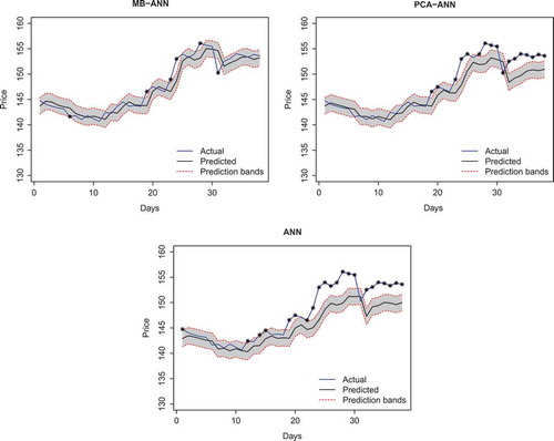
We will call the proportion of the $Y_t$s in the prediction band the in-band rate. Among the 38 new data points, the in-band rates with the band with $2\hat{\sigma }$ are 0.842 for MB-ANN, 0.553 for PCA-ANN, and 0.421 for ANN. The results indicate that the predictions based on MB-ANN are more accurate than those of PCA-ANN and ANN.

Results Based on S&P 500

We extended the previous result to the 488 companies in the Standard & Poor’s 500 index (S&P 500) and compared the prediction performance of the three methods, ANN, MB-ANN, and PCA-ANN. For the analysis on each of the companies, we used the same initial values and conditions for estimation such as the time order, the number of hidden layer, and the number of neurons in the hidden layer, as those used for Apple Inc..

It is interesting to see that the size of Markov blanket varies across the companies from 1 to 4, while the number of the main principal components is 2 for all the companies. The sizes of Markov blanket for all the S&P 500 companies are summarized in Table 6.

Table 6. Markov blanket sizes for the S&P500 companies.

Markov blanket sizes	1	2	3	4
Number of companies	400	64	18	6

The three methods are compared in the context of prediction accuracy, where the predictions are for the 38-day period as was made for Apple Inc.. The comparison was made using the in-band rate and it turns out that our proposed method, MB-ANN, outperformed the others.

Let ${\beta }_l(x)$ be the proportion of the companies that whose in-band rate with the band-width $l\hat{\sigma }$ is larger than or equal to $x$. Then, a higher $\beta$ value means a higher accuracy in prediction. The comparison is summarized in Figure 6, where the $Y$-axis is of ${\beta }_l$ values with the in-band rates on the $X$-axis. We can see that the ${\beta }_l$ values are in general larger by the MB-ANN than those by the other two. For instance, among the 488 stocks in S&P500, ${\beta }_1(0.6)$ is 0.871 (425 stocks) for MB-ANN, 0.824 (402 stocks) for PCA-ANN, and 0.787 (384 stocks) for ANN.

Figure 6. Prediction performance for S&P500 stocks. The $Y$-axis is of ${\beta }_l$ values with the in-band rates on the $X$-axis.

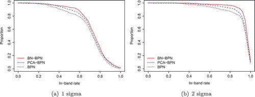
A general indication in the figure is that the prediction accuracy improves in the order of ANN, PCA-ANN, and MB-ANN. The proportions (${\beta }_l$) of stocks whose in-band rates are not smaller than 0.4, 0.6, 0.8, 0.9, and 1 are listed in Table 7. Note in the table that the difference in the ${\beta }_l$ value among the three methods is more conspicuous when $l=1$ than when $l=2$. This implies that the prediction band by the MB-ANN is constructed so that it contains more high-density areas of the distribution of the actual closing values than the prediction bands constructed by the other methods.

Table 7. The proportion (${\beta }_l$) of stocks whose in-band rates are not smaller than 0.4, 0.6, 0.8, 0.9, and 1. The numbers in the bracket indicate the ratios to the result of the ANN.

Band-width	Methods	${\beta }_l$
		0.4	0.6	0.8	0.9	1
1 $\hat{\sigma }$	MB-ANN	0.955 (1.059)	0.871 (1.107)	0.254 (1.239)	0.068 (1.838)	0.016
	PCA-ANN	0.941 (1.043)	0.824 (1.047)	0.237 (1.156)	0.055 (1.486)	0.014
	ANN	0.902 (1.000)	0.787 (1.000)	0.205 (1.000)	0.037 (1.000)	0.000
2 $\hat{\sigma }$	MB-ANN	0.996 (1.022)	0.980 (1.044)	0.959 (1.111)	0.871 (1.190)	0.115 (1.597)
	PCA-ANN	0.988 (1.013)	0.969 (1.032)	0.918 (1.064)	0.779 (1.064)	0.100 (1.389)
	ANN	0.975 (1.000)	0.939 (1.000)	0.863 (1.000)	0.732 (1.000)	0.072 (1.000)

Discussions and Concluding Remarks

In this work, we applied a structure learning method for Bayesian networks in search of informative input variables for a target variable. A main idea in the learning is that we use a mutual information score such as the Kullback–Leibler divergence measure between variables to measure between-variable dependency. The variables whose dependency levels a higher are more likely to be the input variables. Once these informative variables are selected, they form a Markov blanket for the target variable and are used as input variables for our ANN. In this context, we call it MB-ANN.

The results in Table 5 show that our method has a smaller RMSPE in the test set and has a higher RMSPE in the training set. This connotes that we can avoid overfitting and improve prediction accuracy by the MB-ANN. PCA-ANN also reduces the dimensionality of the input data but it only finds the direction that the data are most spread out so that it may fall short of reflecting relevancy of the selected variables to the target variable up to their full scale. Moreover, it may produce even worse results compared to ANN since it might capture only the linear relationship. MB-ANN performs better in input variable selection by selecting the variable based on the dependency structure among the data and can deal with nonlinear relationships.

From the ${\beta }_l$ values in Table 7, we can observe that the predicted values of MB-ANN are more likely to be closer to the actual stock prices.

It is interesting to see that the number of informative input variables was 1 for 400 out of 488 S&P 500 companies and that the last closing value was the only one chosen. Any additional input variable in this case would do nothing but overfitting which should make the prediction model overly data-ridden. Rather than allowing all the variables available as input, it would be desirable that we select an informative set of the input variables and use it for building an ANN as is proposed in this work.

References

- Bengio, Y., P. Lamblin, D. Popovici, and H. Larochelle. 2007. Greedy layer-wise training of deep networks
- Blum, A., and P. Langley. 1997. Selection of relevant features and examples in machine learning. Artificial Intelligence 97 (1–2):245–71. doi:10.1016/S0004-3702(97)00063-5.
- Box, G. E. P., and G. M. Jenkins. 1976. Time series analysis: Forecasting and control. San Francisco: Holden-Day.
- Cybenko, G. 1989. Approximation by superpositions of a sigmoidal function. Mathematics of Control, Signals, and Systems 2 (4):303–14. doi:10.1007/BF02551274.
- Friedman, N., M. Goldszmidt, and A. Wyner. 1999. Data analysis with Bayesian networks: A bootstrap approach. In Proc. 15th Conference on Uncertainty in Artificial Intelligence, 206–15. San Francisco: Morgan Kaufmann.
- Gel’fand, I. M., and A. M. Yaglom. 1957. Calculation of amount of information about a random function contained in another such function. American Mathematical Society Translations, Series 2 12:199–246.
- Grigoryan, H. 2015. Stock market prediction using artificial neural networks. Case Study of TAL1T, Nasdaq OMX Baltic Stock. Database Systems Journal 4 (2): 14-23.
- Guyon, I., and A. Elisseeff. 2003. An introduction to variable and feature selection. The Journal of Machine Learning Reearch 3:1157–82.
- Hornik, K. 1991. Approximation capabilities of multilayer feedforward networks. Neural Networks 4 (2):251–57. doi:10.1016/0893-6080(91)90009-T.
- Kar, A. 1990. Stock prediction using artificial neural networks. Dept. of Computer Science and Engineering, IIT Kanpur.
- Kohavi, R., and G. John. 1997. Wrappers for feature selection. Artificial Intelligence 97 (1–2):273–324. doi:10.1016/S0004-3702(97)00043-X.
- Koller, D., and M. Sahami. 1996. Toward optimal feature selection. In Proceedings of the 13th International Conference on Machine Learning, Bari, Italy, 284 – 92.
- Margaritis, D., and S. Thrun. 1999. Bayesian network induction via local neighborhoods. Advances in Neural Information Processing Systems 12: 505–11.
- May, R., G. Dandy, and H. Maier. 2011. Review of input variable selection methods for artificial neural networks, 19–44. Croatia: Artificial Neural Networks – Methodological Advances and Biomedical Applications.
- Pakdaman, M., H. Taremian, and H. B. Hashemi. 2010. Stock market value prediction using neural networks, In International Conference on CISIM, 132–36. IEEE.
- Riedmiller, M., and H. Braun. 1992. Rprop A fast adaptive learning algorithm. International Symposium on Computer and Information Sciences, VII, November, Antalya.
- Rumelhart, D. E., G. E. Hinton, and R. J. Williams. 1986. Learning representations by back-propagating errors. Nature 323:533–36. doi:10.1038/323533a0.
- Scutari, M., and R. Nagarajan. 2013. Identifying significant edges in graphical models of molecular networks. 57:207–17. doi:10.1016/j.artmed.2012.12.006.
- Tsamardinos, I., C. F. Aliferis, and A. Statnikov. 2003. Algorithms for large scale Markov blanket discovery. In Proceedings of the 16th International Florida Artificial Intelligence Research Society Conference. 376–81, St. Augustine, Fla, USA.
- Werbos, P. 1990. Backpropagation through time: What it does and how to do it. Proceedings of the IEEE 78 (10):1550–60. doi:10.1109/5.58337.
- Whittle, P. 1951. Hypothesis testing in time series analysis. Almquist and Wicksell, Uppsala.
- Zekic, M. 1998. Neural network applications in stock market predictions: A methodology analysis. Proceedings of the 9th International Conference on Information and Intelligent Systems, Varazdin, Croatia, 255–63.