A Multi-Objective Integer Melody Search Algorithm

ABSTRACT

There are a number of algorithms for the solution of continuous optimization problems. However, many practical design optimization problems use integer design variables instead of continuous. These types of problems cannot be handled by using continuous design variables-based algorithms. In this paper, we present a multi-objective integer melody search optimization algorithm (MO-IMS) for solving multi-objective integer optimization problems, which take design variables as integers. The proposed algorithm is a modified version of single-objective melody search (MS) algorithm, which is an innovative optimization algorithm, inspired by basic concepts applied in harmony search (HS) algorithm. Results show that MO-IMS has better performance in solving multi-objective integer problems than the existing multi-objective integer harmony search algorithm (MO-IHS). Performance of proposed algorithm is evaluated by using various performance metrics on test functions. The simulation results show that the proposed MO-IMS can be a better technique for solving multi-objective problems having integer decision variables.

Introduction

In the literature, a number of algorithms are available for the solution of continuous-space optimization problems. However, very often only integer variables occur in practical design optimization problems. Moreover, these optimization problems can have multiple conflicting objectives. As such situations often occur in practice, there is need to have efficient methods to solve these types of problems. In this section, first the basic concepts used in solving multi-objective optimization problem are briefly discussed. Engineering design multi-objective optimization involving integer variable may be stated as a minimization of $M$ components of a vector function $F(\mathbf{x})$ with respect to a vector variable $\mathbf{x}$ in a design space $S$. It can be expressed in mathematical form as follows:

$minF\left(\mathbf{x}\right)=[F_1(\mathbf{x}),F_2(\mathbf{x}),\dots ,F_m(\mathbf{x})]$

$\mathbf{x}=[x_1,x_2,\dots \dots ..,x_n]$

where $F_n(\mathbf{x})$ represents the $n$th objective.

Researchers are continuously developing powerful and effective optimization methods inspired by nature (Karaboga and Akay 2009). The methods involving stochastic search are very popular for solving optimization problems (Karaboga and Basturk 2007). Many meta-heuristic algorithms, such as genetic algorithm, particle swarm optimization (PSO), tabu search, ant colony optimization, and simulated annealing (SA), etc., have been widely employed for various optimization problems. A relatively new meta-heuristic technique, named as harmony search (HS) algorithm, has been proposed by Geem, Kim, and Loganathan (2001), inspired by the music improvisation process. Initially, these algorithms were designed for continuous problems with single objectives. However, latter these algorithms were modified for integer variable case and multi-objective optimization problems.

Inspired by basic concepts applied in HS algorithm, Ashrafi and Dariane (2011) have developed an optimization algorithm called melody search (MS) algorithm. MS is based on musician group performance processes. The MS algorithm proposed by Ashrafi and Dariane (2011) is designed for single-objective optimization problem with continuous variables. In this paper, we have proposed a multi-objective integer melody search (MO-IMS) algorithm to solve multi-objective problems having integer design variables.

This paper is organized as follows. A review of various optimization algorithms for solving integer variable optimization problems is reported in Section 2. A detailed summary on MS algorithm is presented in Section 3. The proposed MO-IMS algorithm is discussed in Section 4. In Section 5, performance metrics for evaluating performance of the algorithm are discussed. Simulation setup and results are discussed in Section 6. Sensitivity analysis of algorithm parameter is provided in Section 7. Finally, concluding remarks are reported in Section 8.

Related Work

Several optimization algorithms are already developed to solve integer variable optimization problems. Some of these optimization algorithms deal with one objective, while the other optimization algorithms can solve multi-objective optimization problems. A brief review of several algorithms is presented in this section.

SA is a stochastic algorithm which have the ability to solve continuous and discrete optimization problems. Kirkpatrick (1984) presented modified SA for combinatorial optimization. They discussed the algorithm computational efficiency by applying it to the travel salesman problems. Furthermore, Cardoso et al. (1997) presented SA algorithm approach to solve mixed integer nonlinear (MINLP) problems. They applied the proposed algorithm to solve several test functions dealing with single-objective optimization.

Deep et al. (2009) proposed a real-coded genetic algorithm named as MI-LXPM for solving integer and mixed integer optimization problems. Their algorithm is an extended version of LXPM. Ocenasek and Schwarz (2002) developed a new variant of estimation of distribution algorithm (EDA) to solve mixed continuous-discrete optimization problems. Rao and Xiong (2005) developed a hybrid genetic algorithm for solving mixed-discrete nonlinear design optimization. They used genetic algorithm to determine the optimal feasible region that contains the global optimum point. To find the final optimum solution, hybrid negative subgradient method integrated with discrete one-dimensional search was subsequently used. Furthermore, Rao and Xiong (2005) suggested the harmony element algorithm (HEA), which combines the principles of the HS algorithm and the GA. HEA works for continuous variables.

Laskari, Parsopoulos, and Vrahatis (2002) investigated performance of PSO variants for integer programing problems. They compared PSO performance with well-known Branch and Bound technique on several test problems. Results indicated that PSO clearly has better performance than Branch and Bound techniques. Geem, Kim, and Loganathan (2001) presented HS algorithm for discrete variables. The methods involving HS algorithm have been applied to various problems from structural design to solving Sudoku puzzles, from musical composition to medical imaging, and from heat exchanger design to course timetabling. Geem (2005) firstly adopted the standard HS with binary-coding (BHS) to solve water pump switching problems by discarding the pitch adjustment operator. Then Geem and Williams (2008) utilized BHS to solve an ecologic optimization problem and achieved better results than those using the SA algorithm.

Geem (2008) introduced the novel stochastic partial derivative for discrete decision variables. A new HS algorithm was presented for solving mixed-discrete optimization problems. Jaberipour and Khorram (2011) presented a new HS algorithm for solving mixed-discrete engineering optimization problems. They presented a mixed-discrete HS approach for solving these nonlinear optimization problems which contain integer, discrete, and continuous variables. Wang et al. (2010) presented a discrete binary harmony search (DBHS) algorithm for solving binary problems. They developed a new pitch adjustment rule for DBHS to enhance the optimization capability of HS. Results show that DBHS outperformed the discrete PSO algorithm and standard HS algorithm. Furthermore, they extended DBHS to solve the Pareto-based multi-objective optimization problems (Wang et al. 2011). Moreover, Wang et al. (2013) presented modified version called an improved adaptive binary search algorithm (ABHS). They used different benchmark functions and 0–1 knapsack problem to evaluate the performance of ABHS.

Kong et al. (2015) developed a simplified binary harmony search (SBHS) algorithm to tackle 0–1 knapsack problems, which is an important subset of combinatorial optimization. Results from SBHS show that it can obtain better solutions than most well-known state-of-the-art HS methods including nine continuous versions and five binary-coded variants. According to Ashrafi and Dariane (2011), the MS algorithm finds better solution than genetic algorithm (GA), PSO, artificial bee colony (ABC), and HS algorithms. The current MS algorithm is applicable only to problems with continuous variables, and it handles only single-objective optimization problems. Therefore, in this paper, we propose an MO-IMS algorithm for solving the multi-objective optimization problems having integer variables more efficiently and effectively.

Melody Search Algorithm

Ashrafi and Dariane (2011) developed a new meta-heuristic algorithm inspired by the HS algorithm inspired by musical performance process where group of musicians attempt to find better series of pitches in melodic line. In this algorithm, named as MS algorithm, group music improvisation processes have been mathematically modeled for solving single-objective optimization problem. MS adopts the basic concepts applied in HS algorithm but its structure is different. Each melodic pitch represents a decision variable of the real problem and each melody represents a solution of the optimization problem. Unlike single-harmony memory as in HS, MS algorithms have several memories. Each of these memories is called as Player Memory (PM). Hence, several solutions are generated and evaluated in the same computational step. Several series of pitches are performed each time while each player sounds a series of pitches within the melodic line. An interactive relation between players enhances efficiency of MS algorithm. Each player sounds a series of pitches within their possible ranges, and if succession of pitches makes a good melody, then that melody is stored in the PM. Then melodic improvisation step for each PM is performed. There are two phases in the MS algorithm: in the first phase, each music player can improvise his/her melody without the influence of others, while in the second phase, the algorithm acts as a group performance by interactions of several players.

Proposed Multi-Objective Integer Melody Search (MO-IMS) Algorithm

To solve multi-objective problems having integer variables, Pareto dominance scheme along with new improvisation process is incorporated in the proposed MO-IMS algorithm. The two important concepts used in multi-objective optimization are Pareto dominance and Pareto optimality.

Pareto Dominance

Given two candidate solutions ${\mathbf{x}}_{\mathbf{1}}$ and ${\mathbf{x}}_{\mathbf{2}}$ from S, vector F(${\mathbf{x}}_{\mathbf{1}}$) is said to dominate vector F(${\mathbf{x}}_{\mathbf{2}}$) (denoted by F(${\mathbf{x}}_{\mathbf{2}}$) $\prec$ F(${\mathbf{x}}_{\mathbf{1}}$) if and only if,

(1) $F_i({\mathbf{x}}_{\mathbf{1}})\le F_i({\mathbf{x}}_{\mathbf{2}}),\mathrm{\forall }i\in \left\{1,....,m\right\}$(1)

(2) $F_i({\mathbf{x}}_{\mathbf{1}})<F_i({\mathbf{x}}_{\mathbf{2}}),\mathrm{\exists }i\in \left\{1,....,m\right\}$(2)

If solution ${\mathbf{x}}_{\mathbf{1}}$ is not dominated by any other solution, then ${\mathbf{x}}_{\mathbf{1}}$ is declared as a nondominated or Pareto optimal solution. There may be other equally good solutions but not superior than ${\mathbf{x}}_{\mathbf{1}}$.

Pareto Optimality

The candidate solution ${\mathbf{x}}_{\mathbf{1}}$ $\in$ S is Pareto optimal if and only if,

(3) $F({\mathbf{x}}_{\mathbf{2}})\prec F({\mathbf{x}}_{\mathbf{1}}),\mathrm{\neg }\mathrm{\exists }{\mathbf{x}}_{\mathbf{2}}\in \mathrm{S}$(3)

Solutions that satisfy (3) are known as Pareto optimal solutions and Pareto front is obtained from fitness objective function values corresponding to these solutions.

The parameters defined in MS algorithm are number of player memories (PMN), player memory size (PMS), maximum number of iterations for the initial phase (NII), maximum number of iterations (NI), and player memory considering rate (PMCR).

Algorithm 1 MO-IMS: Pseudo code of multi-objective integer melody search optimization

Initialize Parameters {PMS, PMN, PMCR, PAR, NVAR, NI and NII}

First Phase

1: for $\mathrm{P}\mathrm{M}\mathrm{N}$ times do

2: Melody Memory initialization

3: for $\mathrm{P}\mathrm{M}\mathrm{S}$ times do

4: PM $\leftarrow$ {new random melodic vector x with fitness F}

5: end for

6: end for

7: repeat {

8: start of improvisation process

9: for $\mathrm{j}\mathrm{f}\mathrm{r}\mathrm{o}\mathrm{m}1\mathrm{t}\mathrm{o}\mathrm{N}\mathrm{V}\mathrm{A}\mathrm{R}$ times do

10: Memory consideration

11: if rand()$<$ PMCR then

12: index $\leftarrow$ int(rand()*PMS)+1

13: for $\mathrm{i}\mathrm{f}\mathrm{r}\mathrm{o}\mathrm{m}1\mathrm{t}\mathrm{o}\mathrm{P}\mathrm{M}\mathrm{N}$ times do

14: $x_i^{\prime }=\mathrm{P}\mathrm{M}(\mathrm{i}\mathrm{n}\mathrm{d}\mathrm{e}\mathrm{x},\mathrm{i})$$▹$ selection from melody memory

15: end for

16: Pitch adjustment

17: if rand()$<$PAR then

18: if rand()$<$0.5 then

19: if index$>$1 then

20: $\mathrm{i}\mathrm{n}\mathrm{d}\mathrm{e}\mathrm{x}\leftarrow \mathrm{i}\mathrm{n}\mathrm{d}\mathrm{e}\mathrm{x}-1$

21: for $\mathrm{i}\mathrm{f}\mathrm{r}\mathrm{o}\mathrm{m}1\mathrm{t}\mathrm{o}\mathrm{P}\mathrm{M}\mathrm{N}$ times do

22: $x_i^{\prime }\leftarrow \mathrm{P}\mathrm{M}(\mathrm{i}\mathrm{n}\mathrm{d}\mathrm{e}\mathrm{x},\mathrm{i})$

23: end for

24: else

25: break

26: end if

27: else

28: if index$<$PMS

29: $\mathrm{i}\mathrm{n}\mathrm{d}\mathrm{e}\mathrm{x}\leftarrow \mathrm{i}\mathrm{n}\mathrm{d}\mathrm{e}\mathrm{x}+1$

30: for $\mathrm{k}\mathrm{f}\mathrm{r}\mathrm{o}\mathrm{m}1\mathrm{t}\mathrm{o}\mathrm{P}\mathrm{M}\mathrm{N}$ times do

31: $x_i^{\prime }\leftarrow \mathrm{P}\mathrm{M}(\mathrm{i}\mathrm{n}\mathrm{d}\mathrm{e}\mathrm{x},\mathrm{i})$

32: end for

33: else

34: break

35: end if

36: end if

37: else

38: break

39: end if

40: Randomization

41: else

42: $x_i^{\prime }=S_i^L+rand()\ast (S_i^U-S_i^L)$$▹$ random selection from solution space

43: end if

44: end for

45: end of improvisation process

46: F $\leftarrow$fitness(x)

47: update_PM(x,F)

48:} until(NII is reached)

49: while (iteration$<$NI)

50: Second Phase

51: Improvisation of new melody vector from each PM

52: Update_PM $▹$ if applicable update PM with new melody vector

53: Paretofront $\leftarrow$ {pareto front evaluated from new melodic vector’s fitness}

54: define new range for variables

55: end while

56: return Paretofront

The main steps in MO-IMS algorithm are summarized in the following table.

Table

Initializing the optimization problem and adopting algorithm parameters Initial Phase;

2.1. Player memories (PM) initialization

2.2. New melody improvisation from each PM

2.3. Updation of each PM

2.4. Repetition of sub-steps 2.2 and 2.3 until the criterion for stopping the initial phase is satisfied

Second phase

3.1. New melody improvisation from each PM according to the possible range of pitches

3.2. Updation of each PM

3.3. For randomization, determine the possible ranges of pitches for the next improvisation

3.4. Repeat sub-steps 3.1, 3.2, and 3.3 until the stopping criterion for the algorithm is satisfied

The first step comprises of initializes the parameters PMN, PMN, PMCR, NII, and NI. It is mentioned in start of Algorithm 1.

Each music player searches the best arrangement of pitches in the melody separately in the first phase. Lines 2–6 of Algorithm 1 specify this step. In the primary part of the initial phase, the player memories are initialized. Melody memory (MM) has several player memories:

(4) $MM=[P{M}_1,P{M}_2,....,P{M}_{PMN}]$(4)

where

(5) $P{M}_i=\left[\begin{array}{ccccc}{x}_{i,1}^1& x_{i,1}^2& ..& x_{i,1}^D& F_i^1\\ x_{i,2}^1& x_{i,2}^2& ..& x_{i,2}^D& F_i^2\\ :& :& ..& :& \hspace{0.17em}\\ x_{i,PMS}^1& x_{i,PMS}^2& ..& x_{i,PMS}^D& F_i^{PMS}\end{array}\right]$(5)

(6) $x_{i,j}^k=L{B}_k+(U{B}_k-L{B}_k)$(6)

where $i=[1,...,PMN]j=[1,...,PMS],k=[1,...,D]$

where D is the number of decision variables and [$L{B}_k,U{B}_k$] is the range of $k^{th}$ variable, which is not changed in the initial phase but is changed in the second phase.

In the second phase, a new melody vector is improvised for each PM. The new vector of decision variables from each PM, $X_{i,new}=\left(x_{i,new}^1,x_{i,new}^2,...,x_{i,new}^D\right)$ is generated from improvisation rule that consists of the following three parts

• • Memory consideration For selection of every element of new melody vector for each player, player memory consideration rate (PMCR) decides whether it should be selected from corresponding PM or from the solution space as follows:

  (7) $x_{i,new}^k=\left\{\begin{array}{cc}{x}_{i,1}^k,x_{i,2}^k,...,x_{i,PMS}^k& \mathrm{w}\mathrm{i}\mathrm{t}\mathrm{h}\mathrm{p}\mathrm{r}\mathrm{o}\mathrm{b}\mathrm{a}\mathrm{b}\mathrm{i}\mathrm{l}\mathrm{i}\mathrm{t}\mathrm{y}\mathrm{P}\mathrm{M}\mathrm{C}\mathrm{R}\\ x_{i,new}^k\in \mathbf{S}& \mathrm{w}\mathrm{i}\mathrm{t}\mathrm{h}\mathrm{p}\mathrm{r}\mathrm{o}\mathrm{b}\mathrm{a}\mathrm{b}\mathrm{i}\mathrm{l}\mathrm{i}\mathrm{t}\mathrm{y}(1-\mathrm{P}\mathrm{M}\mathrm{C}\mathrm{R})\end{array}\right.$(7)

where $k=1,2,...,D$

• ○ Pitch adjustment After memory consideration, value of the currently selected element in the new melody vector is checked for possible pitch adjustment as follows:

  (8) $\mathrm{P}\mathrm{i}\mathrm{t}\mathrm{c}\mathrm{h}\mathrm{a}\mathrm{d}\mathrm{j}\mathrm{u}\mathrm{s}\mathrm{t}\mathrm{i}\mathrm{n}\mathrm{g}\mathrm{d}\mathrm{e}\mathrm{c}\mathrm{i}\mathrm{s}\mathrm{i}\mathrm{o}\mathrm{n}\mathrm{f}\mathrm{o}\mathrm{r}{x}_{i,new}^k\leftarrow \left\{\begin{array}{c}\mathrm{Y}\mathrm{e}\mathrm{s}\mathrm{w}\mathrm{i}\mathrm{t}\mathrm{h}\mathrm{p}\mathrm{r}\mathrm{o}\mathrm{b}\mathrm{a}\mathrm{b}\mathrm{i}\mathrm{l}\mathrm{i}\mathrm{t}\mathrm{y}\mathrm{P}\mathrm{A}\mathrm{R}\\ \mathrm{N}\mathrm{o}\mathrm{w}\mathrm{i}\mathrm{t}\mathrm{h}\mathrm{p}\mathrm{r}\mathrm{o}\mathrm{b}\mathrm{a}\mathrm{b}\mathrm{i}\mathrm{l}\mathrm{i}\mathrm{t}\mathrm{y}(1-\mathrm{P}\mathrm{A}\mathrm{R})\end{array}\right.$(8)

where $k=1,2,...,D$

If pitch adjustment decision is yes, then the corresponding neighbor value is selected.

• • Random selection

  With probability (1-PMCR), values for new melodic vector are randomly selected from the given ranges of variable.

Melody improvisation process is described in lines 8–45 of Algorithm 1.

Updation of each PM: In this step, melody memory is updated based on the fitness value of the newly generated melody vector. If fitness value of newly generated melody vector is better than the fitness value of any of the vector already stored in the melody memory then, that vector is replaced by the new melody vector.

Possible ranges of variables for next improvisation: In the second phase, for the next improvisation process, new possible ranges of variables are calculated. This step is used to increase the possibility of composing a better melody vector in the second phase:

(9) $\begin{array}{c}\mathbf{f}\mathbf{o}\mathbf{r}k=1,...,\mathrm{D}times\mathbf{d}\mathbf{o}\\ \mathrm{L}{{\mathrm{B}}_{\mathrm{k}}}^l=min(x_{1,\mathrm{k}},...,x_{PMN,k})\\ \mathrm{L}{{\mathrm{B}}_{\mathrm{k}}}^u=max(x_{1,k},...,x_{\mathrm{P}\mathrm{M}\mathrm{N},\mathrm{k}})\\ \mathbf{e}\mathbf{n}\mathbf{d}\end{array}$(9)

Performance Metrics

Several performance metrics are used to evaluate the performance of the MO-IMS algorithm. Here we used the following performance metrics to compare the performance of MO-IMS algorithm with multi-objective IHS algorithm.

Overall Nondominated Vector Generation (${\mathit{V}}_{\mathit{n}\mathit{d}}$)

This metric shows how many nondominated solutions an algorithm finds in a particular run (Van Veldhuizen and Lamont et al. 2000). If we represent the computed nondominated solution set with Q and the true Pareto-optimal set with P. Then, ideally overall nondominated vector generation of Q is equal to the total number of solutions in P. It is denoted by $V_{nd}$

(10) $V_{nd}=|Q{|}_c$(10)

where ${\left|.\right|}_c$ is cardinality operator.

Overall Nondominated Vector Generation Ratio ($\mathit{V}{R}_{nd}$)

This is the ratio of N (the number of solutions in Q) to the number of solutions in $P$. It indicates how close the computed and true Pareto fronts are to each other (Van Veldhuizen and Lamont et al. 2000):

(11) $V{R}_{nd}=\frac{V_{nd}}{P}$(11)

The value of $V_{nd}$R varies between 0 (worst) and 1 (best).

Error Ratio (${\mathit{E}}_{\mathit{r}}$)

It is a relative error ratio of the set Q with respect to the set P. It indicates how many solutions in the computed Pareto front set Q are not in the true Pareto front set P knowles2002metrics:

(12) $E_r=\frac{{\sum }_{i=1}^{V_{nd}}{e}_i}{V_{nd}}$(12)

$e_i=\left\{\begin{array}{cc}0& \mathrm{i}\mathrm{f}\mathrm{a}\mathrm{v}\mathrm{e}\mathrm{c}\mathrm{t}\mathrm{o}\mathrm{r}\mathrm{i}\mathrm{n}\mathrm{Q}\mathrm{i}\mathrm{s}\mathrm{a}\mathrm{l}\mathrm{s}\mathrm{o}\mathrm{i}\mathrm{n}\mathrm{P}\\ 1& otherwise\end{array}\right.$

Zero error ratio is the ideal value indicating 100% correspondence between Q and P.

Set Coverage Metric (SCM)

Set coverage metric, as proposed by Zitzler and Thiele (1999), calculates the relative spread of solutions between the computed nondominated solution set(Q) and true Pareto-optimal set($P$):

(13) $C(P,Q)=\frac{|q\in Q;\mathrm{\exists }p\in P:Pq{|}_c}{V_{nd}}$(13)

The metric C(P,Q) calculates the proportion of solutions in Q which are weakly dominated by solutions of P.

Generational Distance (${\mathbf{G}}_{\mathbf{d}}$)

This metric, as suggested by Van Veldhuizen and Lamont et al. (2000), finds the average distance of the computed nondominated solutions from the true Pareto optimal set. It is formulated as follows:

(14) $G_d=\frac{\sqrt{\sum _{i=1}^N{d}_i^2}}{N}$(14)

where N represents the number of computed nondominated solutions and $d_i$ is the Euclidean distance from the ith solution($q_i$) to the nearest member of P. $d_i$ can be calculated as follows:

(15) $d_i=\underset{j}{min}\left|q^i-p^j\right|$(15)

where $q_i$ is the $i$th solution Q and $p^j$ is the $j$th member of P.

Maximum Pareto-Optimal Front Error ($\mathit{M}\mathit{P}\mathit{F}\mathit{E}$)

Van Veldhuizen and Lamont et al. (2000) also proposed maximum Pareto-optimal front error as another performance metric. This metric gives the maximum error band that, when considered with respect to Q, covers every solution in $P$. This is basically the maximum value of $d_i$ from Equation 15. It is calculated by the following equation:

(16) $MPFE=\underset{j}{max}\left(\begin{array}{c}\underset{j}{min}\left|q^i-p^j\right|\end{array}\right)=\underset{i}{max}(d_i)$(16)

where $q_i\in Q$ and $p^j\in P$. Ideal value of this metric is zero. This metric gives a broad idea on the closeness of Q to the $P$.

Spacing ($\mathit{S}$)

This metric, proposed by Schott in 1995, gives the measure of closeness of the solutions to the uniformly spread and is calculated with a relative distance measure between consecutive solutions in Q:

(17) $S=\sqrt{\frac{1}{V_{nd}}\sum _{i=1}^{V_{nd}}{(d_i-\hat{d})}^2}$(17)

where $V_{nd}$ is same as in Equation 1, $d_i=\underset{k}{min}\left\{\sum _{i=1}^M\left|q_m^i-q_m^k\right|\right\}$, $k=1,2,...,V_{nd}$ and $i\ne k$. $M$ is the number of objectives being optimized and $\hat{d}$ is the mean of all $d_i$. $q$ in $d_i$ is a solution from set Q. An algorithm having a smaller value of $S$ is better in terms of uniformly spread.

Spread ($\mathit{S}p$)

Zitzler, Deb, and Thiele (2000) proposed a metric which measures the extent of spread in the computed solution set Q which they formulated as follows:

(18) $Sp=\frac{\sum _{m=1}^M{d}_m^e+\sum _{i=1}^{V_{nd}}\left|d_i-\hat{d}\right|}{\sum _{m=1}^M{d}_m^e+V_{nd}\ast \hat{d}}$(18)

where ${\mathrm{V}}_{\mathrm{n}\mathrm{d}}$ is the number of solutions in Q, $d_i$ is the distance between neighbor solutions in Q, $M$ is the number of objectives being optimized, and $\hat{d}$ is the mean of all $d_i$. The parameter $d_m^e$ is the distance between the extreme solutions of P and Q corresponding to the $m$th objective.

Simulation Setup and Results

We performed simulation in MATLAB to demonstrate the performance of MO-IMS for two test functions. Results obtained from proposed algorithm are compared with MO-IHS. The MO-IMS algorithm parameters are as follows: PMN = 3, PMCR = 0.9, PAR = 0.9 and rand() is a random number in the range [0,1]. The parameters of MO-IHS are as follows: HMS = 12, HMCR = 0.9, $\mathrm{P}\mathrm{A}{\mathrm{R}}_{\mathrm{m}\mathrm{i}\mathrm{n}}$ = 0.4, $\mathrm{P}\mathrm{A}{\mathrm{R}}_{\mathrm{m}\mathrm{a}\mathrm{x}}$ = 0.9. Pareto front obtained from algorithms are shown for each function. The average and standard deviation of results obtained from 10 independent experiments for all performance metrics are represented in tables. The values in bold font are the best average result with respect to each performance metric in the tables.

Test Function 1

This function was proposed by Deb (1999) as follows:

(19) $\mathrm{F}:\left\{\begin{array}{cc}\mathrm{M}\mathrm{i}\mathrm{n}\mathrm{i}\mathrm{m}\mathrm{i}\mathrm{z}\mathrm{e}& f_1(x_1,x_2)=x_1\\ \mathrm{M}\mathrm{i}\mathrm{n}\mathrm{i}\mathrm{m}\mathrm{i}\mathrm{z}\mathrm{e}& f_2(x_1,x_2)=g(x_1,x_2).h(x_1,x_2)\end{array}\right.$(19)

where

$g(x_1,x_2)=11+x_2^2-10.\mathrm{c}\mathrm{o}\mathrm{s}(2\pi x_2)$

$h(x_1,x_2)=\left\{\begin{array}{cc}1-\sqrt{\frac{f_1(x_1,x_2)}{g(x_1,x_2)}},& \mathrm{i}\mathrm{f}{f}_1(x_1,x_2)\le g(x_1,x_2)\\ 0,& \mathrm{o}\mathrm{t}\mathrm{h}\mathrm{e}\mathrm{r}\mathrm{w}\mathrm{i}\mathrm{s}\mathrm{e}\end{array}\right.$

and $x_1\in [1,100],x_2\in [-300,300]$

For this experiment, total number of iterations is 1000. Figures 1–2 show the obtained Pareto front from MO-IMS and MO-IHS along with true Pareto front, respectively. Continuous line in each picture shows the true Pareto front for test function 1. MO-IMS and MO-IHS are able to obtain nondominated solution along the true Pareto front. The figures show that the proposed MO-IMS algorithm covers the true Pareto front with large number of points (i.e., nondominated solutions) compared to the MO-IHS algorithm.

Figure 1. Pareto front obtained from MO-IMS for test function 1.

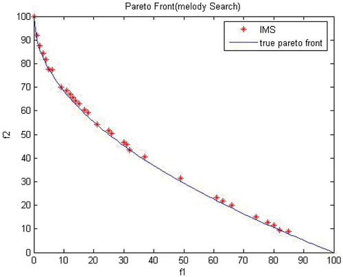
Figure 2. Pareto front obtained from MO-IHS for test function 1.

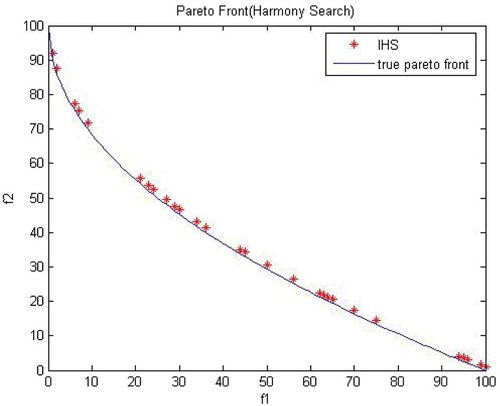
Performance of both algorithms is compared using performance metrics, as shown in Table 1. MO-IMS performs better for generational distance, spacing and maximum Pareto-optimal front error, spread, overall nondominated vector generation, set converge metric, and overall nondominated vector generation ratio metrics. MO-IHS performs better for error ratio metric with respect to mean, MO-IMS perform better than MO-IHS for this metric when considering standard deviation. MO-IMS has an average value of 54.1 for ONVG and 45.5 for SCM performance metrics. This means, on average, MO-IMS results in 54 nondominated points of which 45 points are on the true Pareto front. MO-IHS has an average value of 48.6 for ONVG and 5.8 for SCM metrics. This clearly shows MO-IMS performs better than MO-IHS in terms of ONVG, SCM, and other performance metrics.

Table 1. Performance metric for test function 1.

Algorithm	MO-IMS	MO-IHS
Generational distance
Average	0.2895	1.0704
Standard deviation	0.7397	1.1430
Spacing
Average	1.4001	1.7585
Standard deviation	0.5485	0.7068
Spread
Average	0.4435	0.5102
Standard deviation	0.0824	0.0937
Maximum Pareto-optimal front error
Average	4.5789	10.3491
Standard deviation	9.5345	10.0950
Overall nondominated vector generation
Average	54.1000	48.6000
Standard deviation	7.8804	11.2862
Set converge metric
Average	45.5000	5.8000
Standard deviation	18.7394	18.3412
Overall nondominated vector generation ratio
Average	0.5356	0.4812
Standard deviation	0.0780	0.1117
Error ratio
Average	0.8102	0.1000
Standard deviation	0.3063	0.3162

Test Function 2

This function was proposed by Deb (1999) as follows:

(20) $\mathrm{M}\mathrm{i}\mathrm{n}\mathrm{i}\mathrm{m}\mathrm{i}\mathrm{z}\mathrm{e}=\left\{\begin{array}{cc}{f}_1(x)& =1-\mathrm{e}\mathrm{x}\mathrm{p}\left(-\sum _{i=1}^n{(x_i-\frac{1}{\sqrt{n}})}^2\right)\\ f_2(x)& =1-\mathrm{e}\mathrm{x}\mathrm{p}\left(-\sum _{i=1}^n{(x_i+\frac{1}{\sqrt{n}})}^2\right)\end{array}\right.$(20)

where

$x_i\in [-400,400]$

$i\in [1,n]$

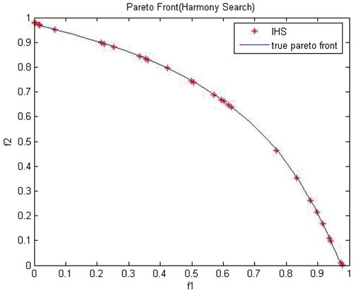
In this experiment, 1000 number of iterations have better result for most of the performance metrics as shown in Table 6. Figures 3–4 show the obtained Pareto front from MO-IMS and MO-IHS along with true Pareto front, respectively. True Pareto front for test function 2 is shown by continuous line in each picture. It can be clearly observed from the figures that the true Pareto front is completely covered by the proposed MO-IMS algorithm with significantly large number of points (i.e., nondominated solutions) compared to the MO-IHS algorithm. Comparison among two algorithms is done by using different performance metrics are shown in Table 2. MO-IMS performs better than MO-IHS with respect to generational distance, spacing, spread, maximum Pareto-optimal front error, set converge metric and error ratio, overall nondominated vector generation and overall nondominated vector generation ratio metrics. MO-IMS has an average value of 149.7 for ONVG and 1 for SCM performance metrics. MO-IHS has an average value of 26.2 for ONVG and 0 for SCM metrics. MO-IMS performs better than MO-IHS for all the performance metrics.

Table 2. Performance metric for test function 2.

Algorithm	MO-IMS	MO-IHS
Generational distance
Average	0.0014	0.0033
Standard deviation	0.0001	0.1099
Spacing
Average	0.0034	0.0336
Standard deviation	0.0005	0.8440
Spread
Average	0.3181	0.7476
Standard deviation	0.0502	0.5322
Maximum Pareto-optimal front error
Average	0.0327	0.0314
Standard deviation	0.0000	5.9136
Overall nondominated vector generation
Average	149.7000	26.2000
Standard deviation	10.4142	12.4405
Set converge metric
Average	1.0000	0
Standard deviation	0.0000	0.8540
Overall nondominated vector generation ratio
Average	5.1621	0.9034
Standard deviation	0.3591	0.4290
Error ratio
Average	0.0067	0
Standard deviation	0.0005	0.4420

Figure 3. Pareto front obtained from MO-IMS for test function 2.

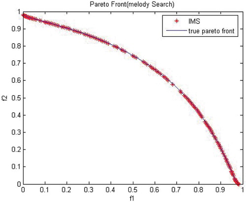
Figure 4. Pareto front obtained from MO-IHS for test function 2.

Sensitivity Analysis

Impact of various algorithm parameters upon performance on MO-IMS is studied in this section. Two experiments are carried out to show the parameters effect on algorithm.

Effect of Variation in Player Memory Size

In this experiment, number of PM size is varied to check the performance of the algorithm via the performance metrics. We perform simulation for three different values of PMS, i.e., 6, 12, and 24. For each PMS, algorithm is run 10 times.

Test Function 1

Table 3 shows that PMS of 24 have best result in all of performance metrics. This shows increasing number of PMS results in better results; however, increasing PMS results in increment in simulation time. Results of PMS of 12 are near to the results of PMS of 24.

Table 3. Effect of variation in PMS for test function 1.

PMS	6	12	24
Generational distance
Average	0.0270	0.0294	0.0264
Standard deviation	0.0440	0.0440	0.0443
Spacing
Average	0.0708	0.0704	0.0654
Standard deviation	0.0550	0.0570	0.0581
Spread
Average	0.7181	0.7045	0.6886
Standard deviation	0.1742	0.1884	0.1744
Maximum Pareto-optimal front error
Average	0.2750	0.3034	0.2721
Standard deviation	0.4616	0.4584	0.4629
Overall nondominated vector generation
Average	16.8500	19.5500	22.7500
Standard deviation	5.1122	7.9636	9.6675
Set converge metric
Average	7.8000	8.9000	9.0000
Standard deviation	8.2437	10.7405	12.3884
Overall nondominated vector generation ratio
Average	0.1685	0.1955	0.2275
Standard deviation	0.0511	0.0796	0.0967
Error ratio
Average	0.4393	0.4039	0.3699
Standard deviation	0.3820	0.3852	0.4065

Test Function 2

With respect to generational distance, spread, spacing, overall nondominated vector generation and nondominated vector generation ratio, error ratio metrics, PMS of 24 has best average result as shown in Table 4. While the PMS of 6 has best average result for set converge metric. For the maximum Pareto front error metrics PMS of 12 has best average result.

Table 4. Effect of variation in PMS for test function 2.

PMS	6	12	24
Generational distance
Average	0.0040	0.0051	0.0013
Standard deviation	0.0004	0.0022	0.0000
Spacing
Average	0.0340	0.0578	0.0031
Standard deviation	0.0067	0.0345	0.0003
Spread
Average	0.4028	0.4637	0.3101
Standard deviation	0.0778	0.1154	0.0255
Maximum Pareto-optimal front error
Average	0.0302	0.0300	0.0327
Standard deviation	0.0028	0.0030	0.0000
Overall nondominated vector generation
Average	16.1000	11.8000	158.3000
Standard deviation	2.1833	4.2635	6.8484
Set converge metric
Average	0.9000	0.6000	0.8000
Standard deviation	0.3162	0.5164	0.4216
Overall nondominated vector generation ratio
Average	0.5552	0.4069	5.4586
Standard deviation	0.0753	0.1470	0.2362
Error ratio
Average	0.0564	0.0486	0.0051
Standard deviation	0.0212	0.0449	0.0027

Observation

The use of PM size of 24 gives better average results for test functions 1 and 2 with respect to most of the performance metrics. Therefore, PM size of 24 is a good choice for the test functions 1 and 2. Generally, the increasing number of PMS results in better results. However, algorithm takes more time by increasing PMS. A larger value of PMS leads to more simulation time and small value of PMS can degrade the performance of algorithm. Therefore, an appropriate value of PMS should be selected according to the problem.

Effect of Variation in Iterations

In this experiment, we varied number of iterations to analyze the effect of variation in iterations number on the MO-IMS algorithm. Different runs with 100, 200, 500, and 1000 number of iterations are carried out, while all the other parameters are kept fixed.

Test Function 1

Table 5 shows the best average results for test function 1. It can be observed that 1000 number of iterations have better result in Generational distance, spacing, spread and maximum Pareto-optimal front error. In case of set converge metric, overall nondominated vector generation and overall nondominated vector generation ratio metrics, 500 number of iterations have better result.

Table 5. Effect of variation in iterations for test function 1.

Iterations	100	200	500	1000
Generational distance
Average	0.2380	0.1958	0.0402	0.0294
Standard deviation	0.2327	0.2087	0.0515	0.0440
Spacing
Average	0.3977	0.2287	0.1275	0.0704
Standard deviation	0.7531	0.1852	0.1819	0.0570
Spread
Average	0.9153	0.8953	0.8294	0.7045
Standard deviation	0.2760	0.2025	0.2951	0.1884
Maximum Pareto-optimal front error
Average	3.1256	2.3044	0.8484	0.3034
Standard deviation	3.3469	1.9309	1.2506	0.4584
Overall nondominated vector generation
Average	19.9500	20.8500	24.6300	19.5500
Standard deviation	6.8937	8.5303	4.6594	7.9636
Set converge metric
Average	0.9000	2.9000	12.4200	8.9000
Standard deviation	2.1981	6.5446	8.6037	10.7405
Overall nondominated vector generation ratio
Average	0.1995	0.2085	0.2463	0.1955
Standard deviation	0.0689	0.0853	0.0466	0.0796

Table 6. Effect of variation in iteration for test function 2.

Iterations	100	200	500	1000
Generational distance
Average	0.0069	0.0095	0.0058	0.0013
Standard deviation	0.0015	0.0056	0.0019	0.0001
Spacing
Average	0.1596	0.1599	0.0928	0.0035
Standard deviation	0.0893	0.1012	0.0724	0.0005
Spread
Average	0.6452	0.7158	0.5489	0.3343
Standard deviation	0.2355	0.1865	0.1857	0.0498
Maximum Pareto-optimal front error
Average	0.0249	0.0399	0.0310	0.0327
Standard deviation	0.0069	0.0329	0.0143	0.0000
Overall nondominated vector generation
Average	5.5000	5.6000	8.7000	151.2000
Standard deviation	1.7795	1.2649	3.6530	8.3506
Set converge metric
Average	0.1000	0.1000	0.4000	0.9000
Standard deviation	0.3162	0.3162	0.5164	0.3162
Overall nondominated vector generation ratio
Average	0.1897	0.1931	0.3000	5.2138
Standard deviation	0.0614	0.0436	0.1260	0.2880

Test Function 2

In this experiment, 1000 number of iterations have better result for most of the performance metrics. Results obtained from 1000 number of iterations for generation distance, spacing, spread, set converge metric, ONVG, and ONVGR are found better as compared to other number of iterations.

Observation

As 1000 iteration proved better average results with respect to most of the performance metrics for the test functions 1 and 2. Therefore, 1000 iterations is suitable choice for these two test functions. Further increase in iterations takes more computational time with little improvement in results. Generally, the performance of the algorithm improves with increasing number of iterations at the cost of increased computational complexity. Therefore, based on the problem in hand, a tradeoff between performance improvement and computational complexity needs to be made.

Conclusion

In this paper, a new MO-IMS algorithm is presented for solving optimization problems having more than one objective and containing integer decision variables. Bi-objective test problems with several performance metrics are used to compare the performance of the proposed MO-IMS algorithm with MO-IHS algorithm. Results show that on average MO-IMS performs better than MO-IHS for almost all the performance metrics. This validates the use of MO-IMS for solving multi-objective integer optimization problems.

References

- Ashrafi, S. M., and A. B. Dariane. 2011. A novel and effective algorithm for numerical optimization: Melody search (MS). In Hybrid Intelligent Systems (HIS), 2011 11th International Conference on, 109–14. Melacca, Malaysia: IEEE Conference.
- Cardoso, M. F., R. L. Salcedo, S. Feyo de Azevedo, and D. Barbosa. 1997. A simulated annealing approach to the solution of MINLP problems. Computers & Chemical Engineering 21 (12):1349–64. doi:10.1016/S0098-1354(97)00015-X.
- Deb, K. 1999. Multi-objective genetic algorithms: Problem difficulties and construction of test problems. Evolutionary Computation 7 (3):205–30. doi:10.1162/evco.1999.7.3.205.
- Deep, K., K. P. Singh, M. L. Kansal, and C. Mohan. 2009. A real coded genetic algorithm for solving integer and mixed integer optimization problems. Applied Mathematics and Computation 212 (2):505–18. doi:10.1016/j.amc.2009.02.044.
- Geem, Z. W. 2005. Harmony search in water pump switching problem. In Advances in natural computation, ed. by L. Wang, K. Chen and Y.S. Ong, vol. 3612, 751–60. Berlin, Germany: Springer.
- Geem, Z. W. 2008. Novel derivative of harmony search algorithm for discrete design variables. Applied Mathematics and Computation 199 (1):223–30. doi:10.1016/j.amc.2007.09.049.
- Geem, Z. W., J. H. Kim, and G. V. Loganathan. 2001. A new heuristic optimization algorithm: Harmony search. Simulation 76 (2):60–68. doi:10.1177/003754970107600201.
- Geem, Z. W., and J. C. Williams. 2008. Ecological optimization using harmony search. In Proceedings of the American Conference on applied mathematics, ed. by C. Long, S.H. Sohrab, G. Bognar and L. Perlovsky, 148–52. Cambridge, MA: World Scientific and Engineering Academy and Society (WSEAS).
- Jaberipour, M., and E. Khorram. 2011. A new harmony search algorithm for solving mixed–discrete engineering optimization problems. Engineering Optimization 43 (5):507–23. doi:10.1080/0305215X.2010.499939.
- Karaboga, D., and B. Akay. 2009. Artificial bee colony (ABC), harmony search and bees algorithms on numerical optimization. Innovative Production Machines and Systems Virtual Conference, Cardiff, UK
- Karaboga, D., and B. Basturk. 2007. A powerful and efficient algorithm for numerical function optimization: Artificial bee colony (ABC) algorithm. Journal of Global Optimization 39 (3):459–71. doi:10.1007/s10898-007-9149-x.
- Kirkpatrick, S. 1984. Optimization by simulated annealing: Quantitative studies. Journal of Statistical Physics 34 (5):975–86. doi:10.1007/BF01009452.
- Knowles, J., and D. Corne. 2002. On metrics for comparing nondominated sets. In Evolutionary Computation, 2002. CEC’02. Proceedings of the 2002 Congress on, vol. 1711–716. Honolulu, HI: IEEE Conference.
- Kong, X., L. Gao, H. Ouyang, and L. Steven. 2015. A simplified binary harmony search algorithm for large scale 0–1 knapsack problems. Expert Systems with Applications 42 (12):5337–55. doi:10.1016/j.eswa.2015.02.015.
- Laskari, E. C., K. E. Parsopoulos, and M. N. Vrahatis. 2002. Particle swarm optimization for integer programming. In Proceedings ofthe 2002 Congress on Evolutionary Computation. CEC'02 (Cat.No.02TH8600),WCCI, vol. 2, 1582–87. Honolulu, HI: IEEE. doi: 10.1109/CEC.2002.1004478
- Ocenasek, J., and J. Schwarz. 2002. Estimation of distribution algorithm for mixed continuous-discrete optimization problems. In 2nd Euro-International Symposium on Computational Intelligence, 227–32. IOS Press
- Rao, S. S., and Y. Xiong. 2005. A hybrid genetic algorithm for mixed-discrete design optimization. Journal of Mechanical Design 127 (6):1100–12. doi:10.1115/1.1876436.
- Van Veldhuizen, David, Gary B Lamont. 2000. On measuring multiobjective evolutionary algorithm performance. In Evolutionary Computation, 2000. Proceedings of the 2000 Congress on, Vol. 1, 204–211. La Jolla, CA: IEEE. doi: 10.1109/CEC.2000.870296
- Wang, L., Y. Mao, Q. Niu, and M. Fei. 2011. A multi-objective binary harmony search algorithm. In Advances in Swarm Intelligence, ICSI 2011. Lecture Notes in Computer Science, ed. by Y. Tan, Y. Shi, Y. Chai and G. Wang, vol. 6729, 74–81. Berlin, Germany: Springer.
- Wang, L., R. Yang, X. Yin, Q. Niu, P. M. Pardalos, and M. Fei. 2013. An improved adaptive binary harmony search algorithm. Information Sciences 232:58–87. doi:10.1016/j.ins.2012.12.043.
- Wang, L., X. Yin, Y. Mao, and M. Fei. 2010. A discrete harmony search algorithm. In Life system modeling and intelligent computing ICSEE 2010, LSMS 2010. Communicationsin Computer and Information Science, ed. by K. Li, X. Li, S. Ma and G.W. Irwin, vol. 98, 37–43. Berlin: Springer.
- Zitzler, E., K. Deb, and L. Thiele. 2000. Comparison of multiobjective evolutionary algorithms: Empirical results. Evolutionary Computation 8 (2):173–95. doi:10.1162/106365600568202.
- Zitzler, E., and L. Thiele. 1999. Multiobjective evolutionary algorithms: A comparative case study and the strength Pareto approach. IEEE Transactions on Evolutionary Computation 3 (4):257–71. doi:10.1109/4235.797969.