Cells to Switches Assignment in Cellular Mobile Networks Using Metaheuristics

ABSTRACT

Cabling, handoff, and switching costs play pivotal roles in the design and development of cellular mobile networks. The assignment pattern consisting of which cell is to be connected to which switch can have a significant impact on the individual cost. In the presence of the limitation on the number of cells that can be assigned to a switch, the problem of the cell to switch assignment (CSA) becomes nondeterministic polynomial time hard to solve with all effective solutions being based on metaheuristic optimization algorithms (MOA) approach. This article applies three recently evolved MOA, namely, flower pollination algorithm (FPA), hunting search (HuS), and wolf search algorithm (WSA) for solving CSA problem. Comprehensive computational experiments conducted to collate the performance of the three algorithms indicate that FPA is superior to both HuS and WSA with respect to attaining the global best value and faster convergence with desired CSA.

Introduction

The mobile station (MS) of a cellular network communicates through a stationary base station (BS) to the mobile switching center (hereafter called as the switch) which routes calls either to another BS or to a public switched telephone network. The cell is defined as the basic geographic unit of a cellular mobile network and is usually represented as hexagons, with the entire cellular mobile network being portrayed as a honeycomb structure. As the distance between a subscriber and the BS increases, the signals between the MS and the BS become weaker while interference from neighboring cells increases. Handoffs are used to avoid the problems associated with weak signals and interference while maintaining mobility. A handoff occurs when a call is transferred automatically by the mobile network from a radio channel in one BS to another radio channel in an adjacent BS as the subscriber crosses into the adjacent BS cell area. As the subscriber advances toward the boundary of the current cell, the call strength dips to a minimum threshold and the MS alerts the network (Pierr and Houéto 2002). The network finds an unused channel on the appropriate adjoining BS and provides the MS with all the information needed for the handoff. The MS then switches to the new channel, usually without the subscriber noticing the transition. The cells among which the handoff frequency is high should be assigned to the same switch as far as possible to reduce the cost of handoffs (Merchant and Sengupta 1995). The endeavor should be to assign cells to switches (determining which cell to be connected to which switch) such that the total cost comprising of cabling cost between cells and switches, handoff cost between adjacent cells and switching cost between two or more switches, is minimized subject to the constraints of the call handling capacities of switches (Menon and Gupta 2004).

The CSA problem was introduced by Merchant and Sengupta (1995) whereby heuristic approach based upon a greedy strategy (denoted as H) was presented while making the observation that optimal approaches fail even with relatively small problem instances. Later, Bhattacharjee, Saha, and Mukherjee (1999) proposed other versions of CSA heuristics (H-II through H-VI). It was found that there was no single heuristic that performed equally well in terms of cost and execution time. Bhattacharjee, Saha, and Mukherjee (2000) solved the problem of balancing traffic (load) amongst switches when the cluster of cells to be connected to a switch is decided during the design of a personal communication service network. Saha, Mukherjee, and Bhattacharjee (2000) proposed a heuristic which was simpler and faster than earlier published results. Mandal, Saha, and Mahanti (2002) employed block depth first search (BDFS) algorithm in which an admissible heuristic was used in order to minimize the paging, updating, and physical infrastructure costs. The same authors in 2004 proposed another heuristic combining BDFS with iterative deepening A* (IDA*) which gave superior results compared to earlier published results in terms of quality of the solution obtained and the execution time to obtain the optimal solution. Approaches based upon metaheuristic optimization algorithms (MOA) (Chawla and Duhan 2014, 2015, Yang 2014) for resolving the CSA problem can also be found in the literature. Various MOA-based approaches to address the above problem include simulated annealing (Menon and Gupta 2004), tabu search (Pierr and Houéto 2002), memetic algorithm (Quintero and Pierre 2002), ant colony optimization (Shyu, Lin, and Hsiao 2004), and modified binary particle swarm optimization (Udgata et al. 2008). All these algorithms except the last one considered the cabling cost and the handoff cost as the cost for assigning cells to the switches. In our approach, switching cost is also added to the total cost in addition to the cabling cost and handoff cost. This paper experimentally demonstrates the application of three recently introduced MOA, namely, flower pollination algorithm (FPA), hunting search (HuS), and wolf search algorithm (WSA) to efficiently solve CSA problem in the cellular mobile network.

Mathematical Problem Formulation

Given a cartel of cells and switches whose positions are established, the CSA problem consists of determining a cell assignment pattern to minimize the cost function, while respecting certain constraints, particularly those related to the capacity of the switches (Menon and Gupta 2004; Udgata et al. 2008). The various notations used are as follows:

$n=$ number of cells;

$m=$ number of switches;

$h_{ij}=$ handoff cost occur between cell $i$ and cell $j$;

$c_{ik}=$cabling cost between cell $i$ and switch $k$;

$d_{ij}=$distance between cell $i$ and switch (MSC) $j$;

$M_k=$call handling capacity of switch $k$;

${\lambda }_i=$ number of communications per time unit in cell $i$.

$y_{ij}=$1, if cells $i$ and j are assigned to same switch.

0 if cells are assigned to different switches.

$x_{ik}=$1, if cell $i$ assigned to switch $k$

0 otherwise.

For all cases, the range of $i$, $j$and $k$ are defined as $1\le i\le n,1\le j\le n,1\le k\le m$

Formulation of Cost Function

The cost function consists of the summation of cabling, handoff, and switching cost. Each one of them is described as follows.

Cabling Cost

Cabling cost depends upon the distance between the base station and switch and number of calls that a cell can handle per unit time. The total cabling cost is given by

(1) ${\sum }_{j=1}^m{c}_{ij}\left({\lambda }_j\right)d_{ij}{x}_{ij}fori=1,2,\dots n$(1)

where $c_{ij}\left({\lambda }_j\right)$ is the cost of cabling per kilometer.It is also modeled as a function of the number of calls that a cell can i handles which is given by

(2) $c_{ij}=A_{ij}+B_{ij}{\lambda }_j$(2)

In Equation (4), A and B are constants whose values are 1 and 0.001, respectively, as reported in the literature (Udgata et al. 2008).

Handoff Cost

Total handoff cost is given by the relation

(3) ${\sum }_{i=1}^n{\sum }_{j=1}^n{h}_{ij}\left(1-y_{ij}\right)$(3)

Two types of handoffs, one which involves only one switch and another which involves two switches, are considered in our approach. When the two cells are assigned to the same switch, the handoff cost is negligible, whereas if the two cells among which handoff takes place are connected to two different switches, handoff cost is quite significant and is calculated using Equation (3).

Switching Cost

The total switching cost involved is defined as

(4) ${\sum }_{i=1}^m{\beta }_i{F}_i\left({\beta }_i\right)$(4)

where ${\beta }_i$ is the total number of calls switch i can handle per unit time and $F_i\left({\beta }_i\right)$ is the cost function of switching a call in switch i. Thus the load at switch i is given by

(5) ${\beta }_i={\sum }_{j=1}^n{\lambda }_j{x}_{ji},foralli=1\dots m$(5)

$F_i\left({\beta }_i\right)$ involves both the cost of switching and the cost of maintaining a call at switch. Thus, $F_i\left({\beta }_i\right)$ can be represented as

(6) $\alpha /\left({\mu }_i-{\beta }_i\right),{\beta }_i<{\mu }_i$(6)

where ${\mu }_i$ denote the call switching capacity of switch i and α is a constant whose value is set at 40 (Udgata et al. 2008).

Total Cost

Total cost is the summation of all three costs .The objective function or the cost function is thus given by

(7) ${\sum }_{j=1}^m{c}_{ij}\left({\lambda }_j\right)d_{ij}{x}_{ij}+\sum _{i=1}^n{\sum }_{j=1}^n{h}_{ij}\left(1-y_{ij}\right)+{\sum }_{i=1}^m{\beta }_i{F}_i\left({\beta }_i\right)$(7)

Constraints of the Problem

The first constraint that should be satisfied is that each cell must be assigned to exactly one switch. This can be expressed as

(8) ${\sum }_{k=1}^m{x}_{ik}=1,1\le i\le m$(8)

The second constraint is that optimization is to be carried out in such a way that the call handling capacity of the switch is not breached. It means that the total load of all the cells which are assigned to a particular switch is below the capacity of the switch. Mathematically it can be represented as

(9) ${\sum }_{i=1}^n{\lambda }_i{x}_{ik}\le M_k,1\le k\le m$(9)

The aim is to minimize Equation (7) subject to the condition that constraints given by Equations (8) and (9) are satisfied.

Methodology

Many algorithms and procedures are available in the literature for finding the solution to Nondeterministic polynomial time (NP) hard problems (Roa 2009, Yang 2010). Some of them are exact methods that are guaranteed to find optimum solutions provided enough time is at hand, while the others are approximation techniques, usually called MOA which will give a good solution to problems within a reasonable amount of time, with no guarantee of achieving optimality (Yang 2014). Given the limitation of exact methods in solving large combinatorial optimization problems (Blum and Roli 2003), approaches based on MOA are often preferred in many practical situations. These emulate the biological, physical,or natural phenomena of the real world (Yang 2015). They usually perform well in most practical situations and have become increasingly popular among researchers in the optimization field (Sutcliffe and Neville 2014). Unlike the deterministic ones, they are derivative-free, competent in solving convex and non-convex problems (Yang 2010), independent of the initial solution, and have the inbuilt inheritance to avoid being trapped in local optimum solutions. However, they have some drawbacks, such as being problem-dependent when it comes to parameter tuning and global solution attainment being not guaranteed. Standard benchmark functions (Jamil and Yang 2013) are typically being employed to determine the overall efficiency of MOA. These algorithms are tested using at least a subset of these benchmark functions with diverse properties so as to make sure that the tested algorithm can solve certain types of optimization problems efficiently. In the present work, the three (FPA, HS, and WSA) MOA employed to solve CSA problem seem to be very promising and have been proven to have excellent convergence characteristics on different benchmark functions. A brief introduction to each of these three algorithms is given below.

Flower Pollination Algorithm (FPA)

FPA is inspired from the pollination process among flowering plants in which the reproduction between flowers takes place by transfer of pollen from one flower to another (Yang 2012). FPA is based on the following four rules (Yang, Karamanoglu, and He 2013).

1. Biotic and cross-pollination can be considered as a process of global pollination, and pollen-carrying pollinators move in a way which obeys Levy flights.

2. For local pollination, abiotic, and self-pollination are used.

3. Pollinators such as insects can develop flower constancy, which is equivalent to a reproduction probability that is proportional to the similarity of two flowers involved.

4. The interaction or switching of local pollination and global pollination can be controlled by a switch probability $p$ ∈ [0, 1], with a slight bias toward local pollination.

In the global pollination step, flower pollen gametes are carried by pollinators such as insects, and pollen can travel over a long distance because insects can often fly and move in a much longer range. This can be represented mathematically as

(10) $x_i^{t+1}=x_i^t+\gamma L\left(\lambda \right)\left(x_i^t-g_{\ast }\right)$(10)

where $x_i^t$ is the pollen $i$ or solution vector $x_i$at iteration $t$, and $g_{\ast }$ is the current best solution found among all solutions at the current generation/iteration. Here $\gamma$ is a scaling factor to control the step size. In addition, L (λ) is the parameter that corresponds to the strength of the pollination, which essentially is also the step size. Since insects may move over a long distance with various distance steps, Levy flight can be used to mimic this characteristic efficiently. Levy distribution for L > 0 is given by

(11) $L\sim \frac{\lambda \mathrm{\Gamma }(\lambda )sin(\pi \lambda /2)}{\pi }\frac{1}{S^{1+\lambda }},(S>>S_0>0)$(11)

Here, Γ (λ) is the standard gamma function, and this distribution is valid for large steps s > 0.

Local pollination and flower constancy, can be mathematically represented as

(12) $x_i^{t+1}=x_i^t+ϵ\left(x_j^t-x_k^t\right)$(12)

where $x_j^t$ and $x_k^t$ are pollen from different flowers of the same plant species. This essentially mimics the flower constancy in a limited neighborhood. If $x_j^t$ and $x_k^t$ comes from the same species or selected from the same population, this equivalently becomes a local random walk if $ϵ$ is drawn from a uniform distribution in [0, 1].

Though flower pollination activities (Yang 2014) can occur at all scales, both local and global, adjacent flower patches or flowers in the not-so-far-away neighborhood are more likely to be pollinated by local flower pollen than those far away. In order to copycat this, a switch probability $p$ is used to switch between common global pollination to intensive local pollination. The pseudocode of FPA can be summarized as

Objective min or max$f\left(x\right)$, $x={\left(x_1\dots .x_d\right)}^T$

Initialize a population of n flowers/pollen gametes with random solutions

Find the best solution $g_{\ast }$ in the initial population

Define a switch probability p ∈ [0, 1]

Define a stopping criterion (either a fixed number of generations/iterations or accuracy)

while $\left(t<MaxGeneration\right)$

for i = 1: n (all n flowers in the population)

if $rand<p$,

Draw a (d-dimensional) step vector L which obeys a Levy distribution

Global pollination via $x_i^{t+1}=x_i^t+L\left(g_{\ast }-x_i^t\right)$

else

Draw $ϵ$ from a uniform distribution in [0, 1]

Do local pollination via $x_i^{t+1}=x_i^t+ϵ\left(x_j^t-x_k^t\right)$

end if

Evaluate new solutions

If new solutions are better, update them in the population

end for

Find the current best solution $g_{\ast }$

end while

Output the best solution found

Hunting Search (Hus)

This MOA simulates the behavior of animals hunting in a group (lions, wolves, etc.). Group hunters encircle the prey and gradually tighten the ring of siege until they catch the prey. In addition, each member of the group corrects its position based on its own position and the position of other members. If the prey escapes from the ring, hunters reorganize the group to siege the prey again. In HuS algorithm, artificial hunters move toward the leader. The leader is the hunter which has the best position at the current stage (the optimum solution among current solutions at hand). It is assumed that the leader has found the optimum point and other members move toward it. If any of them finds a point better than the current leader, it becomes the leader in the next stage (Oftadeh and Mahjoob 2009).

The step by step procedure of the HuS is as follows (Oftadeh, Mahjoob, and Shariatpanahi 2010).

Step 1: Initialize the optimization problem and algorithm parameters.

Step 2: Based on the number of hunters in the group, the hunting group matrix is filled with feasible randomly generated solution vectors. The values of the objective function are computed and the leader (the hunter that has the best position in the group) is defined based on the values of objective functions of the hunters.

Step 3: The new hunters’ positions (new solution vectors) $x^{,}=\left(x_1^{,},x_2^{,},\dots ..x_n^{,}\right)$ are generated by moving toward the leader and is given by

(13) $x_i^{,}=x_i+rand\ast MML\ast \left(x_i^L-x_i\right)$(13)

where $rand$ is a uniform random number which varies between 0 and 1, parameter $MML\in \left(0.05,0.4\right)$ is the maximum movement toward the leader, and $x_i^L$ is the position value of the leader for the $i^{th}$variable. For each hunter, if the movement toward the leader is successful, the hunter stays in its new position. However, if the movement is not successful (its previous position is better than its new position), it comes back to the previous position.

Step 4: As the search process continues, there is a chance for the hunters to be trapped in a local minimum (or a local maximum once our goal is to find the maximum). If this happens, the hunters must reorganize themselves to get another opportunity to find the optimum point. The leader keeps its position and the other hunters randomly choose their positions in the design space by

(14) $x_i^{,}=x_i^L\pm rand\times \left(\mathrm{m}\mathrm{a}\mathrm{x}(x_i\right)-\mathrm{m}\mathrm{i}\mathrm{n}\left(x_i\right))\times \alpha \mathrm{e}\mathrm{x}\mathrm{p}\left(-\beta \times \mathrm{E}\mathrm{N}\right)$(14)

where $\mathrm{m}\mathrm{a}\mathrm{x}\left(x_i\right)$ and $\mathrm{m}\mathrm{i}\mathrm{n}\left(x_i\right)$ are the maximum and minimum possible values of variable $x_i$, respectively. EN counts the number of times that the group has been trapped until this step (i.e. number of epochs until this step). As the algorithm goes on, the solution gradually converges to the optimum point. Parameters α and β are positive real values. They determine the global convergence rate of the algorithm. As the algorithm proceeds, the solution gradually converges into the optimum point.

Step 5: Repeat steps 3–4 until the termination criterion is satisfied.

Wolf Search Algorithm (WSA)

WSA is inspired by the hunting behavior of the wolves. It imitates the way wolves search for food and survive by avoiding their enemies.

It is governed by the following three rules (Tang et al. 2012)

1. Each wolf has a fixed visual area defined by the radius $r$ of the visual range. In $2D$, the coverage area will be a circle by the radius $r$. Each wolf can only sense companions who appear within its visual circle and the step size by which the wolf moves at a time is usually smaller than its visual distance.

2. The fitness of the objective function represents the quality of the wolf’s current position. The wolf always tries to move to better terrain but rather than choose the best terrain it opts to move to better terrain that already houses a companion. If there is more than one better position occupied by its peers, the wolf will choose the best terrain inhabited by another wolf from the given options. Otherwise, the wolf will continue to move randomly in Brownian motion.

3. At some point, it is possible that the wolf will sense an enemy. The wolf will then escape to a random position far from the threat and beyond its visual range.

Pseudocode of WSA as to how algorithm actually functions is described as below

Objective function $f\left(x\right),x={\left(x_1,x_2,\dots \dots .x_d\right)}^T$

Initialize the population of wolves,$x_i\left(i=1,2,\dots .,W\right)$

Define and initialize parameters:

$r=$ radius of the visual range.

$s=$ step size by which a wolf moves at a time.

$\alpha =$ velocity factor of wolf.

$p_a$= a user-defined threshold [0, 1] that determines how frequently an enemy appears

while $\left((t<MaxGeneration\right)$&& stopping criteria not met)

for $i=1:W$//for each wolf

Prey_new_food_initiatively ();

Generate_new_location ();

//check whether the next location suggested by the random number generator is new. If not, repeat generating random location.

if $\left(dist\left(x_i,x_j\right)<r\mathrm{\&}\mathrm{\&}{x}_j\mathrm{i}\mathrm{s}\mathrm{b}\mathrm{e}\mathrm{t}\mathrm{t}\mathrm{e}\mathrm{r}\mathrm{a}\mathrm{s}f\left(x_i\right)<f\left(x_j\right)\right)$

$x_i$ moves toward $x_j$//$x_j$ is a better than $x_i$

else if

$x_i$ = Prey_new_food_passively ();

end if

Generate_new_location ();

if $\left(rand()>p_a\right)$

$x_i=x_i+rand()+v;$//escape to a new position.

end if

end for

end while

For further detailed explanation on WSA readers, refer Fong, Deb, and Yang (2015) and Tang et al. (2012).

Procedure for CSA Problem

Step-by-step procedure for the assignment of cells to switches in an optimum manner using FPA, HuS, and WSA is as follows.

Step 1: Initialize the number of cells, switches, and population size (number of flowers in FPA, number of hunters in HuS, and number of wolves in WSA) in the solution space.

Step 2: Initialize position of cells and switches randomly in the search space and calculate the distance between each cell and switch.

Step 3: For each population member, generate an assigned matrix with cells along column and switches along rows.

Step 4: Obtain a solution matrix from the assigned matrix for each population member satisfying the two constraints as described in Equations (8) and (9).

Step 5: For each population member, calculate the total cost using Equation (7).

Step 6: Find the flower, hunter, and wolf with highest fitness value (He, Chen, and Yao 2015) and save its value and assignment.

Step7: Update the solution with minimum cost (highest fitness value) as obtained in step 6 corresponding to the pseudocode of the respective algorithm.

Step 8: Repeat steps 3–7 for the respective algorithm until the stopping criterion is met.

Step 9: Output minimum cost and the corresponding assignment.

Experimental Results

All the experiments were done on Intel (R) Core(TM) 2.50 GHz i5-2520M processor with 4 GB of RAM and 64-bit operating system. The experiments were implemented in MATLAB programming environment. In order to compare the performance of three algorithms (FPA, HuS, and WSA) in solving the CSA problem, the statistical parameters upon which the comparison have been carried out are global best value (GBV), average value (AV), average CPU time $\left(T_{avg}\right)$, coefficient of variation (CV), and percentage gap (Gap %).

Experiments were conducted with a number of cells varying between 25 and 250 and number of switches varying between 2 and 15.Thus, the search space size was between $2^{25}$and ${15}^{250}$. Three main categories of data (Menon and Gupta 2004, Udgata et al. 2008) were generated, based on the number of cells in the set. The small category comprised of problems involving 25 cells and 50 cells, the medium category comprised of problems involving 100 cells and 150 cells, and the large category comprised of problems involving 250 cells. In each category, five values 2, 3, 5, 10, and 15 were used for the number of switches. Ten data sets each were generated for small and medium categories, while five data sets were generated for large categories. Thus, an overall 25 test cases were investigated.

Each algorithm was run 100 times using randomly generated population sets for each run. The numerical data obtained for GBV, AV, and CV for each of the algorithm has been recorded in Table 1, whereas $T_{avg}\left(seconds\right)$ and Gap (in %) has been enlisted in Table 2. In all experiments in this paper, the values of the common control parameters (Karafotias, Hoogendoorn, and Eiben 2015) of the mentioned algorithms such as the population size, number of iterations and the maximum objective function evaluation number were chosen to be the same. The population size has been fixed as 25, the number of iterations was kept at 500 and the maximum objective function evaluation number was set to 1,250,000. These common control parameter settings are sufficient to compare the performances of MOA for this data set. The values of algorithmic-specific (Sun, Garibaldi, and Hodgman 2012) control parameters of the mentioned algorithms are

Table 1. Comparison of the performances of the FPA, HuS, and WSA for the statistical parameters of GBV, AV, and CV.

	GBV			AV			CV
Cells, switches	FPA	HuS	WSA	FPA	HuS	WSA	FPA	HuS	WSA
25,2	1.6310e+003	2.0491e+003	2.0312e+003	2.0907e+003	2.1534e+003	2.1585e+003	6.5175	2.2335	2.6846
50,2	6.6889e+003	8.5318e+003	8.3582e+003	8.7678e+003	8.7169e+003	8.7008e+003	4.6209	1.0446	1.4813
100,2	2.6814e+004	3.4562e+004	3.4509e+004	3.4843e+004	3.4974e+004	3.4889e+004	4.3705	0.6952	0.6239
150,2	5.6018e+004	7.8008e+004	7.7765e+004	7.8018e+004	7.8739e+004	7.8630e+004	4.2874	0.4407	0.4206
250,2	1.5528e+005	2.1727e+005	2.1710e+005	2.1751e+005	2.1856e+005	2.1830e+005	4.1605	0.2510	0.2348
25,3	2.7179e+003	2.7625e+003	2.7339e+003	2.8835e+003	2.8977e+003	2.8979e+003	3.0027	2.4195	2.6058
50,3	1.0929e+004	1.1418e+004	1.1242e+004	1.1583e+004	1.1675e+004	1.1616e+004	2.7105	1.1466	1.1701
100,3	4.1448e+004	4.5971e+004	4.6023e+004	4.6349e+004	4.6632e+004	4.6615e+004	1.8660	0.6508	0.5603
150,3	9.0992e+004	1.0426e+005	1.0400e+005	1.0445e+005	1.0502e+005	1.0495e+005	1.4068	0.3456	0.4547
250,3	2.7817e+005	2.9027e+005	2.9010e+005	2.8797e+005	2.9160e+005	2.9174e+005	1.3274	0.2232	0.2296
25,5	3.3346e+003	3.3584e+003	3.3446e+003	3.5814e+003	3.5225e+003	3.5494e+003	2.6105	2.0895	2.3188
50,5	1.1796e+004	1.3652e+004	1.3657e+004	1.4047e+004	1.4071e+004	1.3994e+004	2.5442	1.2602	1.0562
100,5	5.0393e+004	5.5345e+004	5.4962e+004	5.6163e+004	5.6077e+004	5.6038e+004	1.5991	0.6319	0.6220
150,5	1.2454e+005	1.2487e+005	1.2513e+005	1.2628e+005	1.2607e+005	1.2611e+005	0.4374	0.3905	0.3607
250,5	3.4542e+005	3.4831e+005	3.4865e+005	3.5052e+005	3.5001e+005	3.5007e+005	0.3400	0.2647	0.2250
25,10	3.7725e+003	3.8683e+003	3.7905e+003	3.9916e+003	3.9442e+003	3.9525e+003	2.6236	2.6087	2.2496
50,10	1.5480e+004	1.5487e+004	1.5486e+004	1.5924e+004	1.5803e+004	1.5729e+004	1.3789	1.3476	1.2460
100, 10	6.2236e+004	6.2432e+004	6.2558e+004	6.3342e+004	6.3166e+004	6.3196e+004	0.5981	0.5896	0.4974
150,10	1.4040e+005	1.4066e+005	1.4064e+005	1.4225e+005	1.4202e+005	1.4207e+005	0.4789	0.3605	0.4599
250,10	3.9159e+005	3.9219e+005	3.9192e+005	3.9457e+005	3.9407e+005	3.9407e+005	0.2741	0.2272	0.2613
25,15	3.9036e+003	3.9119e+003	3.9248e+003	4.1096e+003	4.0277e+003	4.0510e+003	2.5094	2.4062	2.3259
50,15	1.5824e+004	1.5847e+004	1.5840e+004	1.6447e+004	1.6306e+004	1.6284e+004	1.3263	1.3588	1.2681
100,15	6.3359e+004	6.4170e+004	6.4092e+004	6.5553e+004	6.5371e+004	6.5466e+004	0.8540	0.5561	0.6433
150,15	1.4280e+005	1.4612e+005	1.4589e+005	1.4740e+005	1.4712e+005	1.4714e+005	0.5491	0.3317	0.3604
250,15	3.5259e+005	4.0712e+005	4.0591e+005	4.0684e+005	4.0871e+005	4.0865e+005	0.5120	0.1800	0.2413

Table 2. Comparison of the performances of the FPA, HuS, and WSA for the statistical parameters of average CPU time and gap.

	$T_{avg}\left(seconds\right)$			Gap (in %)
Cells, Switches	FPA	HuS	WSA	FPA	HuS	WSA
25,2	3.263857	4.134685	3.411685	15.246	9.8039	11.652
50,2	6.301744	9.247038	9.188868	10.294	3.9493	7.0667
100,2	17.74549	20.10683	17.80048	5.8402	2.9858	3.1752
150,2	28.36563	36.12625	29.82601	3.9338	1.7117	1.9591
250,2	176.5936	324.0907	307.1532	2.5556	1.0474	1.0701
25,3	3.159726	4.654387	4.49937	10.693	9.0729	10.644
50,3	6.899344	8.905475	7.399072	8.5278	5.1484	5.6545
100,3	18.91087	20.98962	19.80865	4.3099	2.9399	2.9752
150,3	28.53683	37.95011	31.63722	3.4306	1.3657	2.0234
250,3	307.5603	579.3916	404.9645	2.1082	0.9777	1.0195
25,5	3.062446	4.509508	4.412539	10.396	8.3657	9.5700
50,5	6.64824	9.510889	8.146577	7.1598	5.9351	5.9741
100,5	16.72039	21.51513	18.51984	4.2430	2.4686	3.2906
150,5	30.801	39.60574	34.75368	2.1184	1.8356	1.9015
250,5	377.87	681.4383	651.6237	1.9934	1.0015	1.0340
25,10	3.475894	5.44875	5.232456	10.376	8.0415	9.5662
50,10	7.707233	10.05682	9.302949	6.7334	6.3155	6.7069
100, 10	19.71924	26.00144	21.84485	3.6909	2.4164	2.4598
150,10	37.71099	45.42736	41.04261	2.0102	1.7673	2.0034
250,10	487.0161	774.2363	751.2216	1.7986	0.9370	1.1812
25,15	3.925584	5.093115	4.868172	10.233	10.172	10.192
50,15	8.480547	10.50166	9.615034	6.9543	6.0465	6.3151
100,15	21.93654	25.76043	23.27259	5.0509	2.8542	3.2199
150,15	44.77273	133.4215	87.64931	3.7856	1.3425	1.7066
250,15	611.5116	829.5295	799.6412	1.2127	0.8351	1.2070

For FPA, $\gamma =0.1;\lambda =1.5;p=0.8$have been used.

For HuS, $\alpha =4;\beta =1;MML\in \left(0.05,0.4\right)$have been used.

For WSA, $\alpha =0.8;p_a=0.2;r=10;s=2.5$have been used.

All the three MOA under investigation always found feasible solutions with objective values close to the optimum solution. For all test cases, FPA yielded superior results with respect to attaining the minimum value of cost function (GBV) and $T_{avg}\left(seconds\right)$ in comparison with the other two algorithms. With exceptions, the time needed for solution tended to increase as the number of cells or the number of switches is increased. FPA converged to the optimum solution in the least amount of $T_{avg}$; WSA was intermediate of the other two whereas HuS was the slowest to arrive at the optimum solution. 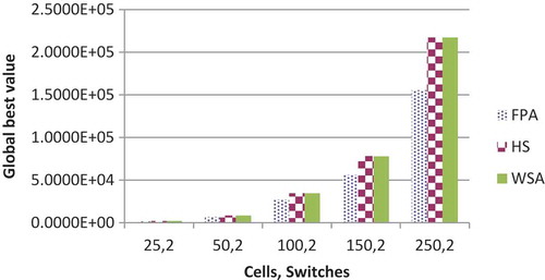The comparative results of three algorithms while considering the $T_{avg}$ for 2, 5, and 15 switches are shown in Figures 1–3, respectively. GBV of HuS and WSA are nearly identical whereas FPA gives the superior performance of the three. It increases with the increase in the number of cell or switches with few exceptions. The comparative results of three algorithms with respect to the GBV for 2, 3, and 15 switches are shown in Figures 4–6, respectively.

Figure 1. Average CPU time comparison between FPA, HuS, and WSA for two switches.

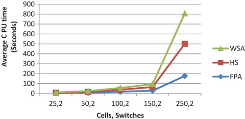
Figure 2. Average CPU time comparison between FPA, HuS, and WSA for five switches.

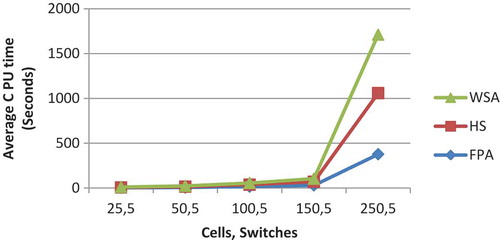
Figure 3. Average CPU time comparison between FPA, HuS and WSA for 15 switches.

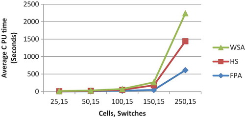
Figure 4. Global best value comparison between FPA, HuS, and WSA for two switches.

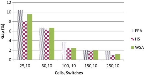
With few exceptions, for all the three algorithms, CV which is calculated as $CV=((standarddeviation/averagevalue)\times 100)$ decreases with the increase in the number of cells or switches. It is a measure of spread that describes the amount of variability relative to the AV. Higher the value of CV, the greater is the dispersion in the variable. It has been found that CV is highest for FPA among all the three algorithms, while that of HuS and WSA are comparable and gives slightly better results than FPA. Comparative results of CV for 3 and 5 switches have been shown graphically in Figures 7 and 8, respectively. For FPA, the value of CV varies from a maximum value of 6.5175 to a minimum value of 0.5120.For HuS, this range varies from 2.2335 to 0.1800, while for WSA, it varies from 2.6846 to 0.2413. Gap (%) is defined as the relative difference between the best and the worst solution. The general trend in all the three algorithms is that the gap reduces with the increase in the number of cells or switches with few exceptions. For all the combination of cells and switches, this gap is highest for FPA. The numerical value of the gap for FPA varies from 15.246% to 1.2127%. For HuS, this range is from 9.8039% to 0.8351% and for WSA it lies between 11.652% and 1.2070%. Comparative analysis of Gap for 3 and 10 switches is shown in Figures 9 and 10, respectively.

Figure 5. Global best value comparison between FPA, HuS, and WSA for three switches.

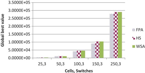
Figure 6. Global best value comparison between FPA, HuS, and WSA for 15 switches.

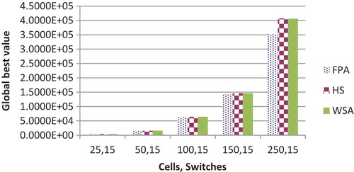
Figure 7. Coefficient of variation comparison between FPA, HuS,and WSA for three switches.

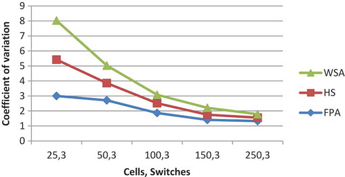
Figure 8. Coefficient of variation comparison between FPA, HuS, and WSA for five switches.

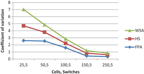
Figure 9. Gap comparison between FPA, HuS, and WSA for three switches.

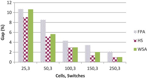
Figure 10. Gap comparison between FPA, HuS, and WSA for 10 switches.

Conclusions

In this paper, we have addressed one of the critical problems concerning how to assign cells to switches to minimize the total cost comprising of cabling, handoff, and switching costs that are usually considered by the designers of cellular mobile networks. We have investigated MOA approaches incorporating FPA, HuS, and WSA for solving the CSA problem. Experiments were performed in MATLAB programming environment whereby a set of experiments were conducted to evaluate the quality of the solutions with respect to the total minimum cost and another set to evaluate the performance in terms of average CPU time to arrive at the solution. All the three algorithms successfully converged to the optimal solution with a desired assignment in a reasonable time, which was practically not possible by traditional mathematical approach due to the huge size of CSA problem. FPA converged to the optimum solution in minimum time and at least cost and thus was superior to both HuS and WSA for the CSA problem under investigation. Empirical results obtained corroborate the proficiency and the effectiveness of MOA to provide good solutions for large-sized cellular mobile networks.

References

- Bhattacharjee, P., D. Saha, and A. Mukherjee. 1999. Heuristics for assignment of cells to switches in a PCSN: A comparative study. Proceedings of the IEEE international conference on personal wireless communications, 331–34. Jaipur, India.
- Bhattacharjee, P., D. Saha, and A. Mukherjee. 2000. CALB: A new cell to switch assignment algorithm with load balancing in the design of a personal communication services network (PCSN). Proceedings of the IEEE international conference on personal wireless communications, Hyderabad, India, 264–68.
- Blum, C., and A. Roli. 2003. Metaheuristics in combinatorial optimization: Overview and conceptual comparison. Journal of ACM Computing Surveys 35:268–308. doi:10.1145/937503.
- Chawla, M., and M. Duhan. 2014. Applications of recent metaheuristics optimization algorithms in biomedical engineering: A review. International Journal of Biomedical Engineering and Technology 16 (3):268–78. doi:10.1504/IJBET.2014.065807.
- Chawla, M., and M. Duhan. 2015. Bat algorithm: A survey of the state of the art. Applied Artificial Intelligence 29 (6):617–34. doi:10.1080/08839514.2015.1038434.
- Fong, S., S. Deb, and X. S. Yang. 2015. A heuristic optimization method inspired by wolf preying behaviour. Neural Computing and Applications 26:1725–38. doi:10.1007/s00521-015-1836-9.
- He, J., T. Chen, and X. Yao. 2015. On the easiest and hardest fitness functions. IEEE Transactions on Evolutionary Computation 19 (2):295–305. doi:10.1109/TEVC.2014.2318025.
- Jamil, M., and X. S. Yang. 2013. A literature survey of benchmark functions for global optimization problems. International Journal of Mathematical Modelling and Numerical Optimisation 4 (2):150–94. doi:10.1504/IJMMNO.2013.055204.
- Karafotias, G., M. Hoogendoorn, and A. E. Eiben. 2015. Parameter control in evolutionary algorithms: Trends and challenges. IEEE Transactions on Evolutionary Computation 19 (2):167–87. doi:10.1109/TEVC.2014.2308294.
- Mandal, S., D. Saha, and A. Mahanti. 2002. A heuristic search for generalized cellular network planning. Proceedings of the IEEE international conference on personal wireless communications, New Delhi, India, 105–09.
- Menon, S., and R. Gupta. 2004. Assigning cells to switches in cellular networks by incorporating a pricing mechanism into simulated annealing. IEEE Transactions on Systems, Man, and Cybernetics—Part B: Cybernetics 34 (1):558–65. doi:10.1109/TSMCB.2003.817081.
- Merchant, A., and B. Sengupta. 1995. Assignment of cells to switches in PCS networks. IEEE/ACM Transaction on Networking 3 (5):521–26. doi:10.1109/90.469954.
- Oftadeh, R., and M. J. Mahjoob. 2009. A new meta-heuristic optimization algorithm: Hunting search. Proceedings of the fifth IEEE international conference on soft computing, computing with words and perceptions in system analysis, decision and control, Famagusta - North Cyprus, 1–5.
- Oftadeh, R., M. J. Mahjoob, and M. Shariatpanahi. 2010. A novel meta-heuristic optimization algorithm inspired by group hunting of animals: Hunting search. International Journal on Computers and Mathematics with Applications 60:2087–98. doi:10.1016/j.camwa.2010.07.049.
- Pierr, S., and F. Houéto. 2002. Assigning cells to switches in cellular mobile networks using taboo search. IEEE Transactions on Systems, Man and Cybernetics—Part B: Cybernetics 32 (3):351–56. doi:10.1109/TSMCB.2002.999810.
- Quintero, A., and S. Pierre. 2002. A memetic algorithm for assigning cells to switches in cellular mobile networks. IEEE Communications Letters 6 (11):484–86. doi:10.1109/LCOMM.2002.805515.
- Roa, S. S. 2009. Engineering optimization theory and practice. 4th ed. Hoboken, New Jersey: John Wiley & Sons, Inc.
- Saha, D., A. Mukherjee, and P. Bhattacharjee. 2000. A simple heuristic for assignment of cells to switches in a PCS network. Wireless Personal Communications 12:209–24. doi:10.1023/A:1008850615965.
- Shyu, S. J., B. M. T. Lin, and T. S. Hsiao. 2004. An ant algorithm for cell assignment in PCS networks. Proceedings of the IEEE international conference on networking, sensing and control, 1081–86. Taipei, Taiwan.
- Sun, J., J. M. Garibaldi, and C. Hodgman. 2012. Parameter estimation using metaheuristics in systems biology: A comprehensive review. IEEE/ACM Transactions on Computational Biology and Bioinformatics 9 (1):185–202. doi:10.1109/TCBB.2011.63.
- Sutcliffe, A. W. C., and R. S. Neville. 2014. Applying evolutionary computing to complex systems design. IEEE Transactions on Systems, Man and Cybernetics—Part A: Systems and Humans 37 (5):770–79. doi:10.1109/TSMCA.2007.902653.
- Tang, R., S. Fong, X. S. Yang, and S. Deb. 2012. Wolf search algorithm with ephemeral memory. Proceedings of the seventh IEEE international conference on digital information management, Macau, China, 165–72.
- Udgata, S. K., U. Anuradha, G. P. Kumar, and G. K. Udgata. 2008. Assignment of cells to switches in a cellular mobile environment using swarm intelligence. Proceedings of the IEEE international conference on information technology, Bhubaneswar, India, 189–94. doi:10.1097/MPA.0b013e31816459b7.
- Yang, X. S. 2010. Engineering optimization: An introduction with metaheuristic applications. Hoboken, New Jersey: John Wiley and Sons, Inc.
- Yang, X. S. 2012. Flower pollination algorithm for global optimization. Unconventional Computation and Natural Computation 7445:240–49.
- Yang, X. S. 2014. Nature inspired optimization algorithms. London: Elsevier.
- Yang, X. S. 2015. Recent advances in swarm intelligence and evolutionary computation, studies in computational intelligence 585. Switzerland: Springer International Publishing.
- Yang, X. S., M. Karamanoglu, and X. He. 2013. Multiobjective flower algorithm for optimization. international conference on computational science, Procedia Computer Science 18, 861–68. Barcelona, Spain: Elsevier.