Support Vector Machine State Estimation

ABSTRACT

The power system state estimator based on the support vector machine (SVM) and the weighted least squares (WLS) method is presented in the paper. The WLS provides state estimations necessary for creating SVM model which is then used for state estimation. The developed algorithm was tested on the IEEE systems, and the performance indicators were calculated in order to compare the accuracy of estimation and the measurement error filtering. The results indicate that the proposed hybrid model outperforms the classical WLS-based state estimation in terms of accuracy and improves measurement error filtering in comparison to the classical estimator.

Introduction

The trend of growing population in developing economies, with goals of reaching already unsustainable energy consumption levels in the countries of a higher living standard, results in increasing energy demands worldwide. As the electric power system forms the backbone of modern lifestyle, special attention should be given to the optimization of its assets and operation. Although the sector of distributed generation was recognized as a potential solution for environmental issues and as a flywheel for stumbled national economies, the intermittent nature of the majority of plants imposes additional uncertainties in power system operation. Furthermore, the electric energy market operations often neglect technical restrictions in favor of a financial profit. Since the obsolete infrastructure was not designed for bidirectional energy and information flows, new concepts and technical solutions are needed in order to assist power utilities worldwide to cope with the challenging trends which result in power systems being operated closer to their stability limits and with lowered security margins.

Figure 3. The estimated states sum of relative variance and relative index change for the IEEE 30.

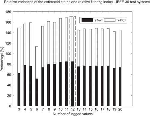
Figure 4. The estimated states sum of relative variance and relative index change for the IEEE 57.

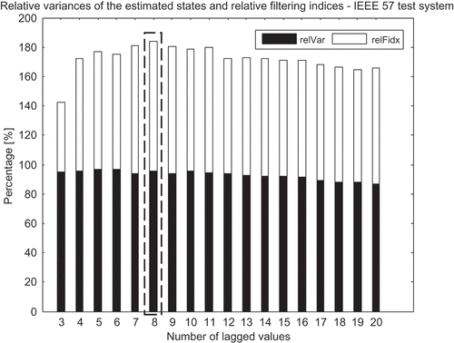
Figure 7. Voltage magnitude estimation errors for the IEEE 14.

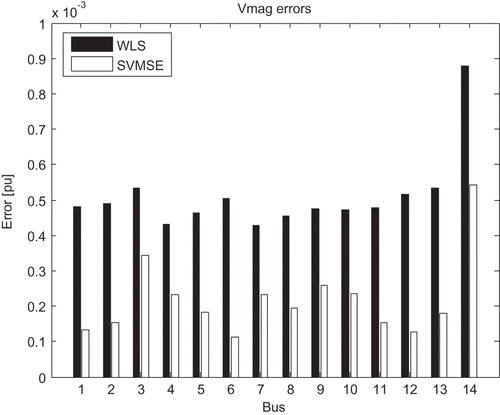
Figure 8. Voltage angle estimation errors for the IEEE 30.

Since it first appeared in the late 1960s (Schweppe, Wildes, and Rom 1970), the state estimator has been playing a significant role in the control centers worldwide as its output is used in the majority of subsequent applications. Therefore, extensive research tackled the field of the state estimation in order to enhance its performance in various aspects (Monticelli 1999; Abur and Gome–Exposito 2004). The emergence of modern sensors offered many benefits in various fields and many numerous were provided in order to optimally combine novel measurements with the conventional supervisory control and data acquisition (SCADA) measurements. Although sensing unit price has continuously been dropping, when it comes to larger power systems, it still presents a financial and a technical challenge to deploy numerous units.

The majority of control centers use the state estimators with the weighted least squares (WLS) method. The problem with WLS estimators based on SCADA measurements is the influence of bad data and imprecise measurements on its accuracy which is, in some cases, significant (Chen and Abur 2006). Different approaches have been suggested to solve this problem, e.g., linear regression (Haughton and Heydt 2013), artificial neural networks (Huang et al. 2010), adaptive Kalman filter (Zhang et al. 2014), etc.

To improve the effectiveness of WLS, a new model that uses an enhanced version of the support vector machine (SVM) algorithm is introduced. Due to the effectiveness in solving different machine-learning problems, such as short-term load forecasting (Ceperic, Ceperic, and Baric 2013), electricity price forecasting (Shiri, Afshar, and Rahimi-Kian 2015), and intrusion detection in SCADA systems (Leandros and Jiang 2014), SVMs have generated a lot of research interest among scientists. Some of the main advantages of SVM are higher tolerance to the increased complexity of the model and lower susceptibility to local minimal. The proposed model improves state estimator performance when compared to a classical WLS-only model.

This paper is organized as follows: The theoretical fundamentals are explained in the section on Theoretical Fundamentals, while the proposed solution is elaborated in the section on Support Vector Machine Theoretical Background. The cases used to test the solution and the obtained results are given in the section on Case Studies. The paper closes with the Conclusion section.

Theoretical Fundamentals

State Estimation Theoretical

Background

The classical state estimation theory, which presents a fundamental for the most of the estimators that run in the control rooms, uses the WLS. The classical state estimation approach is based on SCADA measurements (voltage magnitudes, power flows, and injections) that are combined in the vector of measurements (z), while the vector of state (x) includes phasors of voltage. The relationship between the state vector elements and power flows/injections is:

(1) $z=\mathit{h}(x)+e$(1)

where h(x) contains nonlinear equations, while e denotes errors in measurements. The measurement error covariance matrix denoted as $z=h(x)+e$ (m is a number of measurements and σ is a standard deviation) is used to relate measurement weights to the accuracy of each measurement. The standard uncertainty may be calculated from the accuracy limits A (Al-Othman and Irving 2005; ISO – IEC – OIML – BIPM 2008):

(2) $\sigma =\frac{A}{\sqrt{3}}$(2)

The state estimator results in the optimal estimation by minimizing the objective function J(x):

(3) $\mathit{J}(\mathit{x})=\frac{1}{2}{\left[\mathit{z}-\mathit{h}(\mathit{x})\right]}^T{\mathit{R}}^{-1}\left[\mathit{z}-\mathit{h}(\mathit{x})\right]$(3)

The solution is obtained through an iterative algorithm, with the Gain matrix G(x) and the Jacobian matrix H(x), respectively:

(4) $\mathit{G}(\mathit{x})={\mathit{H}}_{\hspace{0.17em}}^T(\mathit{x})\cdot {\mathit{R}}^{-1}\cdot \mathit{H}(\mathit{x})$(4)

(5) $\mathit{H}(\mathit{x})=\mathrm{\partial }\mathit{h}(\mathit{x})/\mathrm{\partial }\mathit{x}$(5)

The change in the state vector is recalculated until the maximum change $\mathrm{\Delta }{\mathit{x}}^k$becomes smaller than the predefined tolerance:

(6) $\mathit{G}({\mathit{x}}^k)\mathrm{\Delta }{\mathit{x}}^k={\mathit{H}}_{\hspace{0.17em}}^T({\mathit{x}}^k)\cdot {\mathit{R}}^{-1}\left[\mathit{z}-\mathit{h}({\mathit{x}}^k)\right]$(6)

(7) $\mathrm{\Delta }{\mathit{x}}^k={\mathit{x}}^{k+1}-{\mathit{x}}^k$(7)

The issue of the Gain matrix ill-conditioning, caused by the high weights of the measurements such as zero-injections (Abur and Gome–Exposito 2004), is dealt with by introducing a set of constraints:

(8) $\begin{array}{rl}& L(\mathit{x},\mathit{\lambda })\mathbf{=}\frac{1}{2}\mathbf{[}\mathit{z}\mathbf{-}\mathit{h}(\mathit{x}){\mathbf{]}}^T{\mathit{R}}^{-1}\mathbf{[}\mathit{z}\mathbf{-}\mathit{h}(\mathit{x})\mathbf{]}-{\mathit{\lambda }}^T\mathit{c}(\mathit{x})\\ & subjectto\mathit{c}(\mathit{x})=\mathbf{0}\end{array}$(8)

That is minimized by using $\mathrm{\partial }L(\mathit{x},\mathit{\lambda })/\mathrm{\partial }\mathit{\lambda }=0$ and$\mathrm{\partial }L(\mathit{x},\mathit{\lambda })/\mathrm{\partial }\mathit{x}=0$. The system is solved for Δx and λ (the vector of the Lagrange multipliers):

(9) $\left[\begin{array}{cc}\alpha {\mathit{H}}_{\hspace{0.17em}}^T{\mathit{R}}^{-1}\mathit{H}& {\mathit{C}}_{\hspace{0.17em}}^T\\ \mathit{C}& \mathbf{0}\end{array}\right]\left[\begin{array}{c}\mathbf{\Delta }\mathit{x}\\ -\mathit{\lambda }\end{array}\right]=\left[\begin{array}{c}\alpha {\mathit{H}}_{\hspace{0.17em}}^T{\mathit{R}}^{-1}(\mathit{z}-\mathit{h}({\mathit{x}}^k))\\ -\mathit{c}({\mathit{x}}^k)\end{array}\right]$(9)

where $\mathrm{\Delta }\mathit{x}={\mathit{x}}^{k+1}-{\mathit{x}}^k$, $\mathit{C}=\mathrm{\partial }\mathit{c}(\mathit{x})/\mathrm{\partial }\mathit{x}$, and $\alpha =1/max(diag({\mathit{R}}^{-1}))$are the scaling factors used to minimize the Gain matrix condition number.

Support Vector Machine Theoretical Background

This subsection summarizes the support vector regression (SVR) algorithm. The SVMs were introduced by Cortes and Vapnik (1995) with the intention to be used in solving learning problems in regression and classification in a supervised manner.

SVMs were originally applied to classification problems (Cortes and Vapnik 1995) and then later even to regression problems (Drucker et al. 1996). Due to some theoretical guarantees, SVM provides great generalization properties in various classification and regression problems.

The formulation of SVM regression most commonly used is ε-tube support vector regression (ε – SVR, proposed by Vapnik) (Drucker et al. 1996). The main goal is to determine a linear function f, which has the largest difference ε than all data and simultaneously is flat as possible:

(10) $f\left(\mathit{x}\right)=⟨\mathit{w},\mathit{x}⟩+b,$(10)

where the weight vector is w, x is associated input vector, and $b\in R$ is a constant.

The flatness of the function f presupposes seeking a smaller vector w. One of the ways to obtain flatness is b minimizing the${∥\mathit{w}∥}^2=⟨\mathit{w},\mathit{w}⟩$.

The most common way to calculate weight w is by transferring the SVR optimization problem to dual optimization and then applying quadratic programming.

A kernel function on vectors v and z is the function $K>X\to \mathrm{\Re }.$ which fulfills:

(11) $K(\mathit{v},\mathit{z})=⟨\mathrm{\Phi }\left(\mathit{v}\right),\mathrm{\Phi }\left(\mathit{z}\right)⟩.$(11)

Kernel function transformation input space in high-dimensional feature space and then the standard SVR algorithm can be applied (Smola and Schölkopf 2004). The radial basis function (RBF) is kernel function:

(12) $\begin{array}{rl}& K(\mathit{v},\mathit{z})=exp\left(-\gamma {∥\mathit{v}-\mathit{z}∥}^2\right)\\ & \hspace{0.17em}=exp\left(-\gamma \left(⟨\mathit{v},\mathit{v}⟩+⟨\mathit{z},\mathit{z}⟩-2⟨\mathit{v},\mathit{z}⟩\right)\right),\mathrm{f}\mathrm{o}\mathrm{r}\gamma >0.\end{array}$(12)

The ε-SVR requires the selection of two parameters:

the regularization parameter C,

the ε-tube width,

while RBF requires the selection of the additional parameter γ, in Equation (12).

The library for SVM (LIBSVM) tool (Chang and Lin 2011)-based ε-SVR implementation is used in order to select the parameters, known as hyper-parameters. The selection of hyper-parameters is the most important step in building accurate and robust model. For example, an overfitting phenomenon may appear if the case where the value of hyper-parameter C is too large. The most common method for finding near-optimal parameters is a grid search (GS), as shown in Cao et al. (2007), but the main problem is its time consumption.

Many researchers use the particle swarm optimization (PSO) method for optimization of the hyper-parameters (Ceperic, Ceperic, and Baric 2013; Cao et al. 2007). The main principle of the PSO optimization algorithm is based on the principles of swarm intelligence. The use of PSO enables more accurate and faster identification of near-optimal hyper-parameters compared to the GS method and other conventional methods.

In this paper, for SVM hyper-parameter optimization, the particle swarm pattern search method (PSwarm) is used, a technique inspired by PSO. PSwarm is actually a hybrid algorithm that combines, for global optimization, a heuristic approach (particle swarm) and, for local minimization, more rigorous method (pattern search). The PSwarm was introduced in Vaz and Vicente (2007) where it was shown that PSwarm is very competitive in efficiency and has the best result when compared to other tested global optimization solvers. PSwarm combines the efficiency of PSO global and convergence properties of pattern search.

Support Vector Machine State Estimation

The proposed support vector machine state estimator (SVMSE) is a mixed model that improves the classical WLS model by introducing an additional SVR block. The block diagram of hybrid model for each state is shown in Figure 1. The n past inputs and outputs from the WLS are actually used as inputs for building the additional SVR model. The SVR model is then used to calculate actual states by using actual measurements as inputs. For each state, the separate model is built so the number of models depends on the number of states. The determination of optimal hyper-parameters is done by cross-validation on 200 training samples. Once determined, they are used for building SVR models. All the variables used as input for SVR are normalized in the range [−1 1] as suggested in Ceperic, Ceperic, and Baric (2013).

Figure 1. Support vector regression single state estimator block diagram.

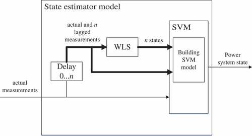
The optimal number of past inputs and outputs used to build an SVR model is determined by optimization on the training data set. The number of optimal past state is actually the number of past states in a given interval for which best results on training data set are obtained.

The advantage of hybrid model is not only in increased performance but also in avoiding the problem of convergence of classical WLS model. In that way, a more robust solution is obtained.

Case Studies

The proposed algorithm was tested on the systems of various topologies, sizes, and locations of measurements (Christie R., Power system test archive; http://www.ee.washington.edu/research/pstca.). The observability analysis was used to ensure the observability. In Tables 1–4, the conventional SCADA measurement locations (buses) are shown.

Table 1. The IEEE 14 SCADA measurements.

Type	Location
Magnitude of voltages	2, 10, 12, 8. 3
Power flows	1–2, 6–13, 7–9, 6–12, 4–9, 5–6, 13–14, 4–7
Power injections	1, 2, 8, 13, 9, 11, 3, 4, 10, 6, 12, 14

Table 2. The IEEE 30 SCADA measurements.

Type	Location
Magnitude of voltages	2, 3, 9, 11, 16, 6, 17, 25, 14, 30
Power flows	1–3, 2–6, 5–7, 6–9, 6–10, 12–13, 14–15, 16–17, 15–18, 10–20, 10–17, 2–4, 15–23, 25–26, 6–8, 25–27, 28–27, 12–15, 4–6, 29–30, 6–28
Power injections	1, 2, 6, 11, 4, 12, 10, 18, 24, 25, 19, 27, 15, 30

Table 3. The IEEE 57 SCADA measurements.

Type	Location
Magnitude of voltages	1, 3, 7, 8, 11, 17, 22, 5, 27, 37, 15, 44, 52, 4, 31, 54
Power flows	1–15, 2–3, 3–4, 4–5, 4–18, 6–7, 7–29, 8–9, 9–10, 9–11, 9–13, 12–16, 12–17, 13–15, 14–15, 18–19, 1–17, 7–8, 22–23, 22–38, 24–25, 14–46, 28–29, 24–26, 26–27, 35–36, 38–48, 9–12, 46–47, 52–29, 32–33, 52–53
Power injections	1, 2, 5, 6, 10, 15, 18, 19, 27, 35, 41, 13, 44, 12, 25, 47, 51, 54, 55, 30, 32, 43, 53, 49, 57

Table 4. The IEEE 118 SCADA measurements.

Type	Location
Magnitude of voltages	4, 12, 25, 36, 73, 10, 76, 27, 86, 40, 107, 59, 111, 82, 92, 112, 18, 117
Power flows	1–2, 3–5, 5–6, 9–10, 5–11, 7–12, 14–15, 16–17, 23–24, 28–29, 30–17, 17–31, 23–32, 34–36, 40–41, 43–44, 2–12, 34–43, 45–49, 52–53, 54–55, 56–57, 50–57, 51–58, 60–62, 64–65, 68–65, 47–69, 71–72, 71–73, 69–75, 4–11, 74–75, 12–14, 76–77, 78–79, 81–80, 77–82, 84–85, 86–87, 85–88, 17–18, 91–92, 92–93, 93–94, 94–95, 82–96, 62–67, 92–100, 95–96, 98–100, 51–52, 99–100, 21–22, 100–101, 6–7, 101–102, 100–106, 105–107, 105–108, 59–60, 39–40, 108–109, 46–48, 103–110, 37–40, 109–110, 110–112, 17–113, 27–115, 114–115, 75–118, 76–118
Power injections	3, 4, 12, 13, 16, 15, 19, 20, 24, 25, 27, 31, 35, 36, 42, 46, 47, 49, 52, 53, 8, 55, 61, 66, 70, 72, 74, 77, 79, 83, 85, 86, 89, 90, 92, 94, 33, 96, 97, 98, 99, 102, 22, 104, 54, 105, 44, 110, 111, 112, 116, 117, 118

The accuracy limits used to calculate the standard uncertainties for each type of measurements are given in Table 5. As the true measurements, the results of power flow calculation were used, while the Gaussian noise was added to simulate the noisy measurements.

Table 5. Maximum measurement uncertainties.

Magnitude of voltages	Power flows	Power injections
0.2%	2%	2%

A total of 1000 trials were run, with randomly generated errors in measurements. The accuracy of the state estimator was expressed through the variance of the estimated states:

(13) ${\sigma }_{\mathrm{\Sigma }}^2=\frac{1}{M}\sum _{i=1}^M\sum _{j=1}^L{\left(\hat{x}{\left(j\right)}_{(i)}-\mathit{x}\left(j\right)\right)}^2$(13)

where ${\hat{x}}_i$ is the vector of estimated states, while x is the vector of true states, M is the number of trials, and L is the number of variables.

The filtering index is calculated as:

(14) $\xi (\hat{x})=\frac{1}{M}\sum _{i=1}^M\frac{\sum _{j=1}^m{({\hat{z}}_j-{\mathit{z}}_j^{\mathrm{t}\mathrm{r}\mathrm{u}\mathrm{e}})}^2}{\sum _{j=1}^m{({\mathit{z}}_j-{\mathit{z}}_j^{\mathrm{t}\mathrm{r}\mathrm{u}\mathrm{e}})}^2}$(14)

where $\hat{z}$ and $z_{\hspace{0.17em}}^{true}$ are the calculated and true values, respectively, while z are measurements containing noise.

For each of the test systems, a base scenario was simulated with 1000 Monte Carlo trials. To determinate systems, SVR hyper-parameters 200 Monte Carlo trials were used, while for finding the optimum number of past n measurements 100 trials were used. Following the calculation of the parameters and number of past measurements for SVR, the test systems were simulated for basic and other operating states in order to test the proposed state estimator performance in various scenarios. Therefore, for each test system, additional scenarios were simulated with a single branch, generator, or load outage, and for each additional scenario, 1000 Monte Carlo trials were carried out.

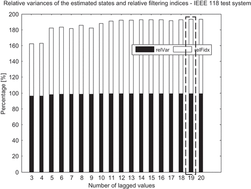
The relative variance and index are calculated as relative change between the variances of the estimated states and the filtering indices of the WLS and SVMSE, expressed in percentage. The sum is obtained as:

(15) $sum=\frac{{\sigma }_{{\sum }^{W}LS}^2-{\sigma }_{\sum SVMSE}^2}{{\sigma }_{\sum WLS}^2}-\frac{\xi {\left(\stackrel{⌢}{x}\right)}_{WLS}-\xi {\left(\stackrel{⌢}{x}\right)}_{SVMSE}}{\xi {\left(\stackrel{⌢}{x}\right)}_{WLS}}$(15)

(16) $sum=relVar+relFidx$(16)

where ${\sigma }_{\sum WLS}^2$ and ${\sigma }_{\sum SVMSE}^2$ are the variances of the estimated states of the models obtained by using expression (13), respectively, while $\xi {\left(\stackrel{⌢}{x}\right)}_{WLS}$ and $\xi {\left(\stackrel{⌢}{x}\right)}_{SVMSE}$ are the filtering indices for the models obtained using expression (14). The optimal number of past values for each test system is determined by selecting the largest relative difference between the WLS and SVMSE models, i.e., the largest sum. Figures 2–5 show the change of the sum of relative variance and relative index for the test systems with different number of past WLS values (lagged values), with the maximum values highlighted in dashed rectangles. The results for the base and the additional scenarios are obtained by simulating the power systems with the given optimal number of state vectors.

Figure 2. The estimated states sum of relative variance and relative index change for the IEEE 14.

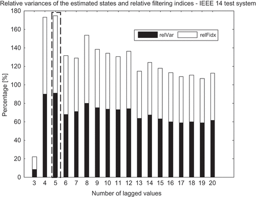
Figure 5. The estimated states sum of relative variance and relative index change for the IEEE 118.

Tables 6–9 show the obtained results for the tests systems when simulating base and additional scenarios, in order to compare the performance of the SVMSE with the classical state estimator.

Table 6. Results for the IEEE 14.

	Classical		SVMSE
System scenario	${\sigma }_{\mathrm{\Sigma }}^2$	$\xi$	${\sigma }_{\mathrm{\Sigma }}^2$	$\xi$
Base scenario	7.2371 × 10^−5	0.4572	6.5621 × 10^−6	0.0725
Branch outage bus #2–#4	7.5969 × 10^−5	0.3104	2.6990 × 10^−5	0.1312
Generator outage bus #2	8.9025 × 10^−5	0.4652	2.9526 × 10^−5	0.2210
Load outage bus #3	3.9402 × 10^−5	0.3876	1.5250 × 10^−5	0.2244

Table 7. Results for the IEEE 30.

	Classical		SVMSE
System scenario	${\sigma }_{\mathrm{\Sigma }}^2$	$\xi$	${\sigma }_{\mathrm{\Sigma }}^2$	$\xi$
Base scenario	3.0474 × 10^−5	0.3622	5.1452 × 10^−6	0.0590
Branch outage bus #2–#6	3.4149 × 10^−5	0.1600	7.7323 × 10^−6	0.0397
Generator outage bus #2	3.4028 × 10^−5	0.3533	7.9799 × 10^−6	0.0867
Load outage bus #5	2.0904 × 10^−5	0.4194	5.3418 × 10^−6	0.1254

Table 8. Results for the IEEE 57.

	Classical		SVMSE
System scenario	${\sigma }_{\mathrm{\Sigma }}^2$	$\xi$	${\sigma }_{\mathrm{\Sigma }}^2$	$\xi$
Base scenario	1.4228 × 10^−5	0.2917	6.4455 × 10^−5	0.0351
Branch outage bus #24–#25	1.0319 × 10^−4	0.3015	1.8631 × 10^−5	0.0622
Generator outage bus #12	1.4882 × 10^−3	0.2534	3.0527 × 10^−4	0.0574
Load outage bus #8	1.4858 × 10^−3	0.2831	2.9687 × 10^−4	0.05765

Table 9. Results for the IEEE 118.

	Classical		SVMSE
System scenario	${\sigma }_{\mathrm{\Sigma }}^2$	$\xi$	${\sigma }_{\mathrm{\Sigma }}^2$	$\xi$
Base scenario	6.4869 × 10^−4	0.7026	5.8957 × 10^−6	0.0421
Branch outage bus #76–#118	1.2280 × 10^−3	0.7063	5.9625 × 10^−6	0.0530
Generator outage bus #49	8.0301 × 10^−4	0.7062	9.0388 × 10^−6	0.0576
Load outage bus #59	5.6933 × 10^−4	0.7002	1.1808 × 10^−5	0.0682

Comparing the results of the SVMSE and the classical state estimator, we can conclude that the accuracy and the measurement error filtering are enhanced since the indices are smaller for the SVMSE in all test scenarios. This is especially true for the base scenario where variances and filtering indices are lower by the order of magnitude. For other scenarios, the results are close or better for SVMSE. The proposed method is faster than the classical approach since the time needed to obtain the state estimate when using the SVMSE is also smaller when compared with the classical state estimator.

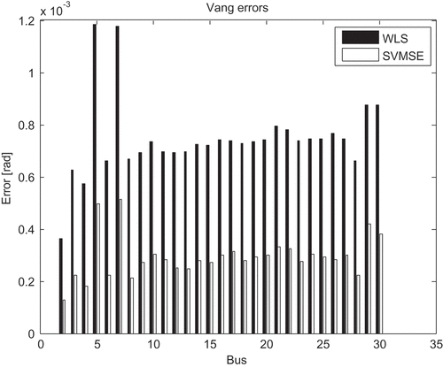
Visual results are given for the base scenario of the IEEE 14 and IEEE 30 test systems only. The estimation errors for these systems are shown in Figures 6–9.

Figure 6. Voltage angle estimation errors for the IEEE 14.

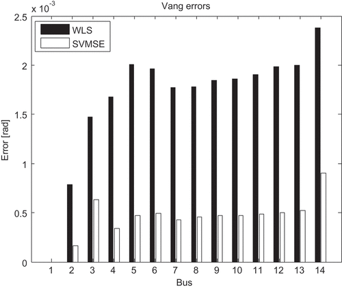
Figure 9. Voltage magnitude estimation errors for the IEEE 30.

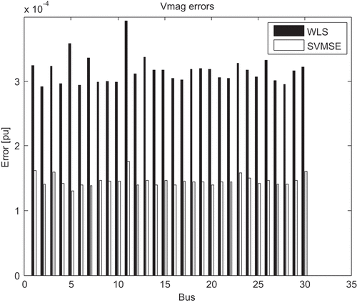
The presented results indicate that the proposed SVMSE estimates voltage angles and magnitudes with smaller errors.

Conclusion

In the paper, the state estimator based on the SVM regression and WLS method is presented. SVR is a machine learning technique known for its good generalization performance, and in this case, it is used to significantly improve the accuracy and effectiveness of the WLS model. The SCADA measurements and states estimated by the WLS model are used as an input of the SVR model. The output of the state estimator is an improved estimation of the complete system.

The algorithm is tested on the IEEE systems, and the performance indicators were calculated in order to compare the accuracy of estimation and the measurement error filtering.

When compared with the WLS-only estimator, it was shown that the proposed model enhances the state estimation accuracy since it provides the estimation of the state vector elements closer to the true values. Furthermore, the measurement error filtering is improved. In addition, the proposed method was shown to outperform the classical one in terms of computational efficiency. Therefore, the proposed method can be utilized as an efficient solution for the power utilities.

Additional information

Funding

This work has been fully supported by the Croatian Science Foundation under the project IP-2018-01-3739 and the University of Rijeka under the projects uniri-tehnic-18-17 & uniri-tehnic-18-15.

References

- Abur, A., and A. Gome–Exposito. 2004. Power system state estimation – Theory and implementation. New York: Marcel Dekker.
- Al-Othman, A., and M. Irving. 2005. Uncertainty modelling in power system state estimation. IET Generation, Transmission & Distribution 152:233–39. doi:10.1049/ip-gtd:20041167.
- Cao, C., J. Xu, Q. Peng, K. Wang, Y. Qiu, Y. Pu, X. Luo, and B. Shuai. 2007. Short-term traffic flow predication based on PSOSVM. Proceeding 1st Int. Conf. Transportation Eng. Amer. Soc. Civil Eng., Chengdu, China, vol. 246, pp. 28–28.
- Ceperic, E., V. Ceperic, and A. Baric. 2013. A strategy for short-term load forecasting by support vector regression machines. IEEE Transactions on Power Systems 28:4356–64. doi:10.1109/TPWRS.2013.2269803.
- Chang, C. C., and C. J. Lin. 2011. LIBSVM: A library for support vector machines. ACM Transaction on Intelligent Systems and Technology 1–27. doi:10.1145/1961189.1961199.
- Chen, J., and A. Abur. 2006. Placement of PMUs to enable bad data detection in state estimation. IEEE Transactions on Power Systems 21:1608–15. doi:10.1109/TPWRS.2006.881149.
- Cortes, C., and V. Vapnik. 1995. Support-vector networks. Machine Learning 20:273–97. doi:10.1007/BF00994018.
- Drucker, H., C. Burges, L. Kaufman, A. Smola, and V. Vapnik. 1996. Support vector regression machines. Advances in Neural Information Processing Systems 9:155–61.
- Haughton, D., and G. Heydt. 2013. A linear state estimation formulation for smart distribution systems. IEEE Transactions on Power Systems 28:1187–95. doi:10.1109/TPWRS.2012.2212921.
- Huang, C., C. Lee, K. Shih, and Y. Wang. 2010. Bad data analysis in power system measurement estimation using complex artificial neural network based on the extended complex kalman filter. European Transactions on Electrical Power 20:1082–100. doi:10.1002/etep.386.
- ISO – IEC – OIML – BIPM. 2008. Guide to the expression of uncertainty in measurement Accessed January 01 2018. https://www.bipm.org/utils/common/documents/jcgm/JCGM_100_2008_E.pdf.
- Leandros, A. M., and J. Jiang. 2014. Intrusion detection in SCADA systems using machine learning techniques. Science and Information Conference (SAI), London, UK, pp. 626–31.
- Monticelli, A. 1999. State estimation in electric power systems – A generalized approach. Massachusetts: Kluwer Academic Publishers.
- Schweppe, F., J. Wildes, and D. Rom. 1970. Power system static-state estimation, parts 1, 2 and 3. IEEE Transactions Power Apparatus and Systems 89:120–35. doi:10.1109/TPAS.1970.292678.
- Shiri, A., M. Afshar, and A. Rahimi-Kian. 2015. Electricity price forecasting using support vector machines by considering oil and natural gas price impacts. IEEE International Conference on Smart Energy Grid Engineering (SEGE), Oshawa, Ontario, Canada, pp. 1–5.
- Smola, A., and B. Schölkopf. 2004. A tutorial on support vector regression. Statistics and Computing 14:199–222. doi:10.1023/B:STCO.0000035301.49549.88.
- Vaz, A., and L. Vicente. 2007. A particle swarm pattern search method for bound constrained global optimization. Journal of Global Optimization 39:197–219. doi:10.1007/s10898-007-9133-5.
- Zhang, J., G. Welch, G. Bishop, and Z. Huang. 2014. A two-stage kalman filter approach for robust and real-time power system state estimation. IEEE Transactions on Sustainable Energy 2:629–36. doi:10.1109/TSTE.2013.2280246.