Self-adaptive Multi-population Rao Algorithms for Engineering Design Optimization

ABSTRACT

The performance of various population-based advanced optimization algorithms has been significantly improved by using the multi-population search scheme. The multi-population search process improves the diversity of solutions by dividing the total population into a number of sub-populations groups to search for the best solution in different areas of a search space. This paper proposes improved optimization algorithms based on self-adaptive multi-population for solving engineering design optimization problems. These proposed algorithms are based on Rao algorithms which are recently proposed simple and algorithm-specific parameter-less advanced optimization algorithms. In this work, Rao algorithms are upgraded with the multi-population search process to enhance the diversity of search. The number of sub-populations is changed adaptively considering the strength of solutions to control the exploration and exploitation of the search process. The performance of proposed algorithms is investigated on 25 unconstrained benchmark functions and 14 complex constrained engineering design optimization problems. The results obtained using proposed algorithms are compared with the various advanced optimization algorithms. The comparison of results shows the effectiveness of proposed algorithms for solving engineering design optimization problems. The significance of the proposed methods has proved using a well-known statistical test known as “Friedman test.” Furthermore, the convergence plots are illustrated to show the convergence speed of the proposed algorithms.

Introduction

The optimization of engineering design problems is a big task for designers and researchers due to the complexity of its mathematical modulation. These design problems contain the mixed type of design variables, i.e., continuous, discrete, and integer variables as well as a number of design constraints which are required to be satisfied for the proper functioning of engineering elements. The researchers are making strenuous efforts for handling such complex requirements of optimization of engineering design problems. The researchers have proposed various metaheuristics (advanced optimization algorithms) to address engineering design problems and to improve their performance. Some of the well-known metaheuristic algorithms are: genetic algorithm (GA), particle swarm optimization (PSO), ant colony optimization (ACO), differential evolution (DE), artificial bee colony (ABC), harmony search algorithm (HSA), simulated annealing (SA), firefly algorithm (FFA), biogeography-based optimization (BBO) gravitational search algorithm (GSA), etc. In addition, various metaheuristics algorithms are proposed in the last decade. Some of them are: spiral optimization, colliding body optimization algorithm, teaching-learning-based optimization (TLBO), cuckoo search (CS) algorithm, differential search algorithm, Jaya algorithm, gray wolf optimization (GWO), galaxy-based search algorithm, crisscross optimization algorithm, cat swarm optimization, ant lion optimization, etc.

The metaheuristic algorithms have their own advantages but most of the optimization algorithms depend on their own algorithm-specific control parameters in addition to common controlling parameters such as the population size and the number of iterations. GA depends on the mutation probability, the selection operator, the crossover probability, etc.; ABC algorithm depends on the number of onlooker bees, scout bees, employed bees, limit, etc.; PSO algorithm depends on its inertia weight, social parameter, cognitive parameter, etc.; HSA depends on number of improvisations, harmony memory consideration rate, etc.; BBO depends on emigration rate, immigration rate, etc. Similarly, other algorithms (except the TLBO algorithm and Jaya algorithm) have their own algorithm-specific control parameters that are to be tuned. The values of algorithm-specificparameters affect the fitness function value(s). The performance of these optimization algorithms gets affected adversely due to improper tuning of the algorithm-specific parameters. The precise tuning of the algorithm-specific control parameters is a tedious process which increases the computational efforts. Due to these reasons, there is a need for the development of new optimization algorithms that are simple to understand and independent of algorithm-specific parameters. Keeping the above points in view, Rao (2020) proposed three Rao algorithms which are simple, algorithm-specific parameter-less and metaphor-less optimization algorithms.

The advanced optimization methods based on the multi-population search process are used for enhancing the search diversity by breaking the total population into a number of sub-population groups and assigning these groups throughout the search space to detect the problem changes effectively. This basic idea is implemented to keep the diversity of the search process by assigning different sub-population groups to different areas of search space. Each population is subjected to either diversifying or intensifying the search processes of the algorithm. A merge and divide process is used for interaction between the sub-populations whenever there is a change in the solution is observed (Rao and Saroj 2017). The multi-population approaches have outperformed the existing fixed population size optimization methods for various problems and these are found effective while dealing with different problems.

Li and Yang (2008) proposed a multi-swarm PSO algorithm and used for solving dynamic optimization problems. Yang and Li (2010) proposed a clustering PSO algorithm for locating and tracking multiple optima in dynamic environments. Zhang and Ding (2011) presented a multi-swarm self-adaptive and cooperative PSO based on four sub-swarm and used to solve complex multimodal benchmark problems. Rao and Patel (2013) proposed multiple teachers based TLBO algorithm and used for optimization of heat exchangers. Xia, Chu, and Geng (2014) proposed a fuzzy c-means multiswarm competitive PSO algorithm and used to realize online operation optimization and control of the chemical process. Turky and Abdullah (2014) proposed a multi-population HSA with external archive for solving dynamic optimization problems. Jena, Thatoi, and Parhi (2015) proposed a dynamically self-adaptive fuzzy PSO technique for smart diagnosis of transverse crack. Gulcu and Kodaz (2015) presented a parallel multi-swarm algorithm based on a comprehensive learning PSO method. Nseef et al. (2016) proposed a multi-population ABC algorithm and used for solving dynamic optimization problems. Wang, Li, and Yang (2017) proposed a self-adaptive DE algorithm with improved mutation mode and used for solving benchmark optimization problems. Rao and Saroj (2017) proposed a multi-population Jaya algorithm and used to solve various unconstrained and constrained benchmark optimization problems.

Zarchi and Vahidi (2018) presented a self-adaptive PSO algorithm to solve the optimization problem of underground cables. Vafashoar and Meybodi (2018) presented a multi-swarm PSO algorithm with adaptive connectivity degree for the particles. Rizk-Allah (2018) optimized engineering design problems using a hybrid sine cosine algorithm with multi-orthogonal search strategy. Zhao et al. (2019) presented an adaptive multi-population non-dominated sorting genetic algorithm and used to optimize multi-objective benchmark problems. Chowdhury et al. (2019) proposed a modified ACO algorithm based on adaptive large neighborhood search to solve a dynamic traveling salesman problem. Mortazavi (2019) proposed a self-adaptive hybrid optimization method which combined the affirmative features of Integrated PSO and TLBO techniques with a fuzzy decision mechanism.

The characteristics of the multi-population optimization approaches are useful because of the following reasons (Li et al. 2015):

1. The overall diversity of the search process can be maintained by allocating the entire population into groups because various sub-populations can be situated in different regions of the problem search space and are having the ability to search in various regions simultaneously.

2. Population-based optimization methods can be easily integrated into other methods.

The number of sub-populations depends on the complexity of the problem. Hence, it is very difficult to decide the number of sub-populations for the effective execution of the algorithm. The incorrect number of sub-populations may also lose the diversity of the search process. In order to avoid these issues, the present work proposes self-adaptive multi-population (SAMP) Rao algorithms to incorporate the advantages of multi-population approach in basic Rao algorithms. The SAMP-Rao algorithms adaptively change the number of subpopulations based on the change in the best fitness value in each iteration in order to control the exploration and exploitation rates of the search process.

The basic objectives of this work are:

1. To propose SAMP-Rao algorithms that split the entire population into the number of sub-populations to improve the diversity of search and change the number of sub-populations adaptively based on the best value of fitness function in each iteration to control the exploration and the exploitation of the search process.

2. To investigate the performance of the proposed algorithms on different benchmark functions and complex engineering design optimization problems.

3. To illustrate the convergence speed of proposed algorithms using convergence plots for problems considered.

The results obtained using the proposed algorithms are compared with various advanced algorithms such as genetic algorithm (GA), particle swarm optimization (PSO), artificial bee colony (ABC), cuckoo search (CS), simulated annealing (SA), moth-flame optimization (MFO), gray wolf optimizer (GWO), ant lion optimizer (ALO), water cycle algorithm (WCA), mine blast algorithm (MBA), evaporation rate water cycle algorithm (ER-WCA), salp swarm algorithm (SSA), whale optimization algorithm (WOA), multi-verse optimization (MVO), and Henry gas solubility optimization (HGSO) algorithm. The computational results of the optimization problems in the present work have revealed that SAMP-Rao algorithms are effective for obtaining highly competitive results compared to the other optimization algorithms reported.

The rest of the paper is structured as section 2 presents description of the proposed SAMP-Rao algorithms, section 3 presents the analysis of computational results obtained using Rao algorithms and proposed SAMP-Rao algorithms for the considered engineering design optimization problems and their comparisons with the results of other optimization algorithms reported, and finally, Section 4 concludes the outcomes of this study.

SAMP-Rao Algorithms

The path of searching an optimal solution using Rao algorithms depends on the best and worst candidate solutions within the entire population and the random interactions between the candidate solutions. Let f is the fitness function which is to be maximized (or minimized). At any iteration w, assume that there are ‘n’ number of populations (i.e., candidate solutions, u = 1,2, …, n) and ‘d’ number of design variables. Let the best value of fitness function f (i.e., f_best) obtains with the best candidate variables, i.e., best within the entire candidate solutions and the worst value of f (i.e., f_worst) obtains with the worst candidate, i.e., worst within the entire population. If X_u,v,w is the value of the vth variable for the uth candidate during the wth iteration, then this value is updated using any one of the following three equations.

(1) $X{ }_{u,v,w}^{\prime }=X_{u,v,w}+r_{1,u,v,w}(X_{best,v,w}-X_{worst,v,w}),$(1)

(2) $\begin{array}{rl}& {X^{\prime }}_{u,v,w}=X_{u,v,w}+r_{1,u,v,w}(X_{best,v,w}-X_{worst,v,w})\\ & +r_{2,u,v,w}(|X_{u,v,w}\mathrm{o}\mathrm{r}{X}_{U,v,w}|-|X_{U,v,w}\mathrm{o}\mathrm{r}{X}_{u,v,w}|),\end{array}$(2)

(3) $\begin{array}{rl}& {X^{\prime }}_{u,v,w}=X_{u,v,w}+r_{1,u,v,w}(X_{best,v,w}-|X_{worst,v,w}|)\\ & +r_{2,u,v,w}(|X_{u,v,w}\mathrm{o}\mathrm{r}{X}_{U,v,w}|-(X_{U,v,w}\mathrm{o}\mathrm{r}{X}_{u,v,w})),\end{array}$(3)

where, X_best,v,w is the value of the best candidate for the variable v and X_worst,v,w is the value of the worst candidate for the variable v during the w^th iteration. X’_u,v,w is the updated value of X_u,v,w and r_1,u,v,w and r_2,u,v,w are the two random numbers for the u^th candidate of vth variable during the w^th iteration in the range [0, 1].

In Equations (2) and (3), the term X_u,v,w or X_U,v,w indicates that the u^th candidate solution is compared with any randomly picked U^th candidate solution and the information is exchanged on the basis of their fitness function values. If the fitness function value of an u^th candidate solution is better than the fitness function value of U^th candidate solution then the term “X_u,v,w or X_U,v,w” becomes X_u,v,w and the term “X_U,v,w or X_u,v,w” becomes X_U,v,w. On the other hand, if the fitness function value of an U^th candidate solution is better than the fitness function value of uth candidate solution then the term “X_u,v,w or X_U,v,w” becomes X_U,v,w and the term “X_U,v,w or X_u,v,w” becomes X_u,v,w.

The searching process of global optimum is carried out using Equations (1)–(3) in Rao-1 algorithm, Rao-2 algorithm, and Rao-3 algorithm, respectively. Equations (1)–(3) can be expressed in a simplified form as,

(4) $x_{new}=x_{old}+r_1\left(x_{best}-x_{worst}\right)$(4)

(5) $x_{new}=x_{old}+r_1\left(x_{best}-x_{worst}\right)+r_2\left(|x_{old}\mathrm{o}\mathrm{r}{x}_{random}|-|x_{random}\mathrm{o}\mathrm{r}{x}_{old}|\right),$(5)

(6) $x_{new}=x_{old}+r_1\left(x_{best}-|x_{worst}|\right)+r_2\left(|x_{old}\mathrm{o}\mathrm{r}{x}_{random}|-\left(x_{random}\mathrm{o}\mathrm{r}{x}_{old}\right)\right)$(6)

Just like the TLBO algorithm (Rao, Savsani, and Vakharia 2011) and Jaya algorithm (Rao 2016, 2019), these three Rao algorithms are also independent of algorithm-specific parameters and thus the efforts of designers are reduced to tune the algorithm-specific parameters for obtaining the best results. Also, the proposed algorithms are comparatively simpler.

In SAMP-Rao algorithms, the following modifications are made to basic Rao algorithms:

1. The proposed SAMP-Rao algorithms use a number of sub-populations by splitting the total population into the number of groups based on the quality of the solutions. The use of the number of sub-populations spread the solutions over the search space rather than focusing on a particular region. Therefore, the proposed algorithms are expected to reach an optimum solution.

2. SAMP-Rao algorithms change the number of sub-populations adaptively during the search process based on the quality of the fitness value. It means that the number of sub-populations will be increased or decreased. This feature supports the search process for searching the optimum solution and for enhancing the diversification of the search process. Furthermore, duplicate solutions are replaced by newly generated solutions to maintain diversity and to enhance the exploration procedure.

The flowchart of the proposed SAMP-Rao-1 algorithm is illustrated in Figure 1. The flowchart of SAMP-Rao-2 and SAMP-Rao-3 algorithm is the same as the SAMP-Rao-1 algorithm except an equation used to modify solutions. In the search process of SAMP-Rao-1 algorithm, solutions modify using Equation (1), whereas, in the case of SAMP-Rao-2 and SAMP-Rao-3 algorithm, solutions modify using Equations (2) and (3) respectively.

Figure 1. Flowchart of the SAMP Rao-1 algorithm.

The basic steps of SAMP-Rao algorithms are as follows:

• Step 1: Initially set the number of populations (P), the number of design variables (d), and termination criterion (for the present work, termination criterion is the maximum number of function evaluations (maxFEs)).

• Step 2: Generate the random initial candidate solutions within the search space.

• Step 3: Divide the entire population into ‘s’ number of groups based on the quality of the solutions (initially s = 2 is considered).

• Step 4: Use one of the Rao algorithms for modifying the solutions in each sub-population group independently. Compare each modified solution with the corresponding old solution and accept if and only if it is better than the old solution.

• Step 5: Merge the entire sub-populations together. Check whether f(best_before) is better than f(best_after).

• Here, f(best_before) is the previous best solution of the entire population and f(best_after) is the current best solution in the entire population. If the value of f(best_after) is better than the value of f(best_before), s is increased by 1 (s = s + 1) to increase the exploration feature of the search process. Otherwise, s is decreased by 1 (s = s - 1) as the algorithm needs to be more exploitive than explorative.

• Step 6: Check the termination criterion. If the search process has reached the maximum number of function evaluations, then terminate the loop and report the best optimum solution. Otherwise, follow the following steps:

1. For re-dividing the population, go to Step 3.

2. Replace the duplicate solutions with randomly generated solutions.

Now, the performance of proposed SAMP-Rao algorithms is tested on 25 unconstrained standard benchmark functions and 14 well-known engineering design optimization problems taken from the literature. The next section presents the analysis of computational results obtained using proposed SAMP-Rao algorithms and its comparison with the results of other algorithms.

Optimization Results and Discussion

The computational experiments are performed using the R2016b version of MATLAB tool. A Laptop with 1.90-GHz Intel Core i3-4030U processor and 8GB RAM is used for computational experiments. The performance of the proposed three algorithms is investigated on 25 unconstrained benchmark problems having different characteristics such as separability, non-separability, unimodality, multimodality, regularity, non-regularity, etc. Furthermore, the performance of the proposed methods is also tested on 14 well-known constrained engineering design optimization problems.

Unconstrained Benchmark Problems

This section presents the analysis of the results of 25 unconstrained benchmark problems presented in Table 35 of Appendix A. The performance of the proposed upgraded version of each Rao algorithm is compared with the corresponding basic Rao algorithms (Rao 2020). The optimization results of proposed algorithms obtained with 500,000 function evaluations over 30 independent runs for each benchmark function are presented in Table 1. The results of Rao algorithms (Rao 2020) for the same benchmark problems are compared with the proposed methods to check for performance improvement.

Table 1. Statistical results of the proposed algorithms over 30 runs for 25 unconstrained benchmark problems considered (500,000 function evaluations).

Function	Optimum		Rao-1*	Rao-2*	Rao-3*	SAMP-Rao-1	SAMP-Rao-2	SAMP-Rao-3
F1	0	B	0	0	0	0	0	0
		W	0	0	0	0	0	0
		M	0	0	0	0	0	0
		SD	0	0	0	0	0	0
		MFE	499976	499791	277522	499896	499760	264470
F2	0	B	0	0	0	0	0	0
		W	0	0	0	0	0	0
		M	0	0	0	0	0	0
		SD	0	0	0	0	0	0
		MFE	499975	499851	276556	499893	499831	275114
F3	0	B	0	0	0	0	0	0
		W	0	0	0	0	0	0
		M	0	0	0	0	0	0
		SD	0	0	0	0	0	0
		MFE	9805	7612	7325	4396	3701	5808
F4	-1	B	-1	-1	-1	-1	-1	-1
		W	0	-1	-1	-1	-1	-1
		M	-0.5667	-1	-1	-1	-1	-1
		SD	0.5040	0	0	0	0	0
		MFE	3010	11187	14025	52166	3110	6627
F5	0	B	0	0	0	0	0	0
		W	0	0	0	0	0	0
		M	0	0	0	0	0	0
		SD	0	0	0	0	0	0
		MFE	77023	110544	143088	27660	41647	55044
F6	0	B	0	0	0	0	0	0
		W	0	5.35E-23	1.32E-25	0	0	0
		M	0	1.80E-24	7.87E-27	0	0	0
		SD	0	9.76E-24	2.61E-26	0	0	0
		MFE	385066	477753	488127	130487	156904	155109
F7	-50	B	-50	-50	-50	-50	-50	-50
		W	-50	-50	-50	-50	-50	-50
		M	-50	-50	-50	-50	-50	-50
		SD	0	0	0	0	0	0
		MFE	17485	37209	34796	16721	32211	32934
F8	-210	B	-210	-210	-210	-210	-210	-210
		W	-210	1171	-210	-210	-210	-210
		M	-210	-30.8587	-210	-210	-210	-210
		SD	0	4.13E+02	0	0	0	0
		MFE	48231	144156	142253	42937	149932	136764
F9	0	B	0	0	0	0	0	0
		W	0	0	0	0	0	0
		M	0	0	0	0	0	0
		SD	0	0	0	0	0	0
		MFE	345615	499767	258451	283000	499707	256045
F10	0	B	0	0	0	0	0	0
		W	0	0	0	0	0	0
		M	0	0	0	0	0	0
		SD	0	0	0	0	0	0
		MFE	301513	499849	144367	352081	263158	130269
F11	0	B	8.95E-26	1.86E-16	1.40E-14	5.64E-13	2.42E-16	2.12E-06
		W	3.9866	22.191719	22.191719	4.04	0.8796	2.373459
		M	0.6644	0.739724	0.739728	1.02	0.1163	0.388004
		SD	1.51E+00	4.05E+00	4.05E+00	1.75	2.36E-01	4.55E-01
		MFE	489811	478410	478420	492722	493267	481648
F12	0	B	0.666667	2.81E-30	0.666667	1.82E-30	1.81E-30	1.81E-30
		W	0.666667	0.666667	0.667019	0.666667	0.666667	0.666667
		M	0.666667	0.288889	0.666686	0.622222	0.222222	0.533333
		SD	0	3.36E-01	7.39E-05	0.169139	0.319642	2.71E-01
		MFE	75427	113638	159231	127503	302529	196018
F13	0.397887	B	0.397887	0.397887	0.397887	0.397887	0.397887	0.397887
		W	0.397931	0.397933	0.397888	0.397888	0.397907	0.397887
		M	0.397892	0.397891	0.397887	0.397887	0.397888	0.397887
		SD	1.05E-05	1.03E-05	1.44E-07	1.96E-07	4.03E-06	1.81E-08
		MFE	102785	41263	80683	39681	28691	80535
F14	0	B	0	0	0	0	0	0
		W	0	0	0	0	0	0
		M	0	0	0	0	0	0
		SD	0	0	0	0	0	0
		MFE	3129	4751	3435	2759	4377	3309
F15	0	B	0	0	0	0	0	0
		W	0	0	0	0	0	0
		M	0	0	0	0	0	0
		SD	0	0	0	0	0	0
		MFE	2963	4272	3191	2535	3795	3061
F16	0	B	0	0	0	0	0	0
		W	0	0	0	0	0	0
		M	0	0	0	0	0	0
		SD	0	0	0	0	0	0
		MFE	4725	12337	6821	4275	10753	2998
F17	0	B	0	0	0	0	0	0
		W	0	0	0	0	0	0
		M	0	0	0	0	0	0
		SD	0	0	0	0	0	0
		MFE	5583	4485	4312	2136	1889	1741
F18	-1.8013	B	-1.801303	-1.801303	-1.801303	-1.801303	-1.801303	-1.801303
		W	-1.801303	-1.801303	-1.801303	-1.801303	-1.801303	-1.801303
		M	-1.801303	-1.801303	-1.801303	-1.801303	-1.801303	-1.801303
		SD	0	0	0	0	0	0
		MFE	3863	2694	2751	3632	2468	2361
F19	-4.6877	B	-4.687658	-4.687658	-4.687658	-4.687658	-4.687658	-4.687658
		W	-4.537656	-3.116841	-3.495893	-4.645895	-4.495893	-4.361327
		M	-4.674306	-4.429948	-4.492183	-4.683482	-4.622998	-4.562120
		SD	3.09E-02	3.60E-01	2.79E-01	1.27E-02	6.51E-02	7.95E-02
		MFE	39710	67252	58401	69443	73844	35037
F20	3	B	3	3	3	3	3	3
		W	3	84	3	3	3	3
		M	3	5.7	3	3	3	3
		SD	0	1.48E+01	0	0	0	0
		MFE	180121	176933	353893	108635	151479	291569
F21	0	B	0	0	0	0	0	0
		W	3.71E-09	0	0	5.95E-11	0	0
		M	1.45E-10	0	0	2.00E-12	0	0
		SD	6.78E-10	0	0	1.09E-11	0	0
		MFE	82792	3139	4453	15931	2916	3245
F22	0	B	1.51E-14	7.99E-15	4.44E-15	1.51E-14	7.99E-15	4.44E-15
		W	2.220970	1.51E-14	1.51E-14	1.340421	1.51E-14	7.99E-15
		M	0.566540	1.04E-14	6.69E-15	0.114229	9.06E-15	5.86E-15
		SD	7.41E-01	3.14E-15	2.38E-15	3.53E-01	2.49E-15	1.77E-15
		MFE	129392	417741	76352	198096	395861	86965
F23	0.998004	B	0.998004	0.998004	0.998004	0.998004	0.998004	0.998004
		W	0.998004	0.998004	0.998004	0.998004	0.998004	0.998004
		M	0.998004	0.998004	0.998004	0.998004	0.998004	0.998004
		SD	0	0	0	0	0	0
		MFE	18839	95983	243748	17505	92195	221936
F24	-3.86278	B	-3.86278	-3.86278	-3.86278	-3.86278	-3.86278	-3.86278
		W	-3.86278	-3.86278	-3.86278	-3.86278	-3.86278	-3.86278
		M	-3.86278	-3.86278	-3.86278	-3.86278	-3.86278	-3.86278
		SD	0	0	0	0	0	0
		MFE	4459	3022	3271	3550	2378	2990
F25	0	B	1.35E-32	1.35E-32	1.35E-32	1.35E-32	1.35E-32	1.35E-32
		W	0.010987	1.597462	0.141320	0.010987	0.054779	0.108359
		M	0.001465	0.057915	0.016008	0.000732	0.004023	0.011303
		SD	3.80E-03	2.91E-01	3.50E-02	2.79E-03	1.06E-02	2.26E-02
		MFE	173661	115593	55637	178127	159795	94663

*The results of Rao algorithms are taken from Rao (2020).

B, best solution; W, worst solution; M, mean solution; SD, standard deviation; MFE, mean function evaluations.

In Table 1, the column named as “optimum” shows the global optimum value of each benchmark function. From Table 1, it can be observed that the statistical results of the SAMP-Rao-1 algorithm are better than Rao-1 algorithms in all benchmark functions except F10 and F11 functions. Also, the statistical results of SAMP-Rao-2 and SAMP-Rao-3 algorithms are better than corresponding Rao-2 and Rao-3 algorithms, respectively. However, the significance of the proposed methods has to be proved using some statistical tests. Hence, a well-known statistical test known as “Friedman test” (Derrac et al. 2011) is used to compare the performance of proposed methods. In this test, initially, the ranking is given to the algorithms in each problem considering statistical results. Rank 1 is given to the algorithm which has obtained the best results and then the ranking of all remaining algorithms in ascending order is done. Finally, the average rank of each algorithm is calculated to get final rank of each algorithm for the considered problems. In this test, the χ² distribution with k-1 degree of freedom is considered (k denotes the number of algorithms considered in test). Friedman test provides the overall performance of each algorithm over the other considered algorithms for the problems considered.

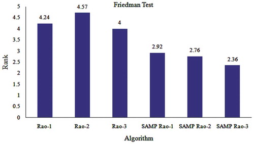
Table 2 presents the average rank of the considered algorithms provided by the Friedman test. The lower value of Friedman rank represents the better performance of the algorithm compared to other algorithms considered. From Table 2, it can be observed that the ranks of SAMP-Rao algorithms are better than the corresponding basic Rao algorithms. Hence, the performance of Rao algorithms is improved by incorporating SAMP approach in these algorithms. The SAMP-Rao-3 algorithm has obtained the first rank among the 6 algorithms with an average score of 2.36. As the p-value of the Friedman test is very less than 0.05, it confirms the high significance of proposed SAMP-Rao algorithms over Rao algorithms for the benchmark problems considered. Figure 2 presents the Friedman rank of algorithms considered on a column chart. From Figure 2, it can be observed that the performance ranking of the algorithms for considered benchmark problems is: SAMP-Rao-3, SAMP-Rao-2, SAMP-Rao-1, Rao-3, Rao-1 and at last Rao-2.

Table 2. Friedman rank test for 25 unconstrained benchmark problems.

Algorithm	Rao-1	Rao-2	Rao-3	SAMP-Rao-1	SAMP-Rao-2	SAMP-Rao-3
Friedman ranks	4.24	4.72	4	2.92	2.76	2.36
χ^2	31.926
p-value	0.00001 (<0.05)

Figure 2. Friedman rank test for 25 unconstrained benchmark problems with 500,000 function evaluations.

Furthermore, the computational complexity of the Rao and SAMP-Rao algorithms is evaluated as shown in Table 3 using guidelines given in the technical report of CEC 2017 (Awad et al. 2016). The computationally expensive Function 18 of CEC 2017 benchmark suite is considered as given in CEC 2017 guidelines to evaluate the computational complexity of the Rao and SAMP-Rao algorithms. The computing time taken by the test program given in CEC 2017 (T₀) is found to be 0.24 s. T₁ is the computing time taken by CEC 2017 benchmark Function 18 for 200,000 function evaluations. T₂ is the total average computing time taken by the algorithm with 200,000 function evaluations over 5 runs. In Table 3, the values of T₃₀/T₁₀ reveal the computational complexity of the algorithms when the dimension of problem changes from 10D to 30D. Similarly, the values of T₅₀/T₁₀ reveal the computational complexity of the algorithms when the dimension of problem changes from 10D to 50D. From Table 3, it can be observed that the complexity of the Rao-1, Rao-2, and Rao-3 algorithms is reduced by 17.33%, 10.5%, and 14.2% using SAMP-Rao-1, SAMP-Rao-2, and SAMP-Rao-3 algorithms, respectively. Similarly, the complexity of the Rao-1, Rao-2, and Rao-3 algorithms is reduced by 10%, 13.83%, and 13.81% using SAMP-Rao-1, SAMP-Rao-2, and SAMP-Rao-3 algorithms, respectively. Hence, the proposed SAMP-Rao algorithms have less computational complexity compared to the Rao algorithms.

Table 3. Computational complexity of the Rao and SAMP-Rao algorithms.

Algorithm	D	T0	T1	T2	TD = (T2-T1)/T0	T30/T10	T50/T10
Rao-1	10	0.24	0.2272	4.808	19.087	2.6518	4.2643
	30	0.24	0.5624	12.7096	50.613
	50	0.24	1.1624	20.6962	81.391
Rao-2	10	0.24	0.2254	5.871	23.523	2.3893	3.8905
	30	0.24	0.5624	14.0516	56.205
	50	0.24	1.14	23.1044	91.518
Rao-3	10	0.24	0.2262	5.9202	23.725	2.4005	3.8371
	30	0.24	0.5728	14.2412	56.952
	50	0.24	1.146	22.9946	91.036
SAMP-Rao-1	10	0.24	0.241	6.6792	26.826	2.1922	3.3524
	30	0.24	0.6	14.7138	58.808
	50	0.24	1.1576	22.741	89.931
SAMP-Rao-2	10	0.24	0.2502	7.559	30.453	2.1385	3.3072
	30	0.24	0.5862	16.2162	65.125
	50	0.24	1.1814	25.353	100.715
SAMP-Rao-3	10	0.24	0.245	7.7316	31.194	2.0595	3.0507
	30	0.24	0.5898	16.0086	64.245
	50	0.24	1.1572	23.9968	95.165

Engineering Design Optimization Problems

In this section, the performance of proposed algorithms is further tested on 14 well-known constrained engineering design problems described in the Appendix B. The performance of the proposed algorithms is compared with the other advanced optimization algorithms such as GA, PSO, ABC, CS, SA, MFO, GWO, ALO, WCA, MBA, ER-WCA, SSA, WOA, MVO, HGSO, and Rao algorithms. For each problem, the results are obtained by executing Rao algorithms and proposed SAMP-Rao algorithms for 50 runs independently. The optimal designs obtained for each problem using each Rao and SAMP-Rao algorithms are tabulated separately and the statistical results of all problems except a spur gear train design problem obtained using SAMP-Rao algorithms over 50 runs are compared with the results obtained using Rao algorithms and the other optimization algorithms. The precision of results up to six decimal points is considered in all problems. A penalty approach is considered to handle constraints in this work. The penalty values are assigned based on fitness values and sensitivity of constraints. In the search process of optimum solution, infeasible solutions that violate the constraint(s) are converted to worse solutions by assigning higher penalties to corresponding fitness values.

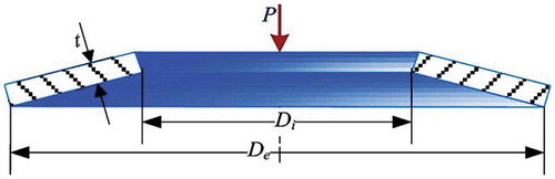
Figure 3 shows the schematic diagram of a Belleville spring. This problem is taken from Yildiz, Abderazek, and Mirjalili (2019) and was initially proposed by Coello (2000). The objective of this problem is the minimization of the weight of spring while satisfying seven non-linear constraints (given as Problem 1 in Appendix B). This problem consists of four continuous type design variables, namely the outer diameter of the spring (D_o), the inner diameter of the spring (D_i), the spring thickness (t), and the spring height (h). The limiting deflection of the spring δ_l depends on the ratio of height to the thickness of the spring.

Figure 3. Schematic diagram of a belleville spring (Yildiz, Abderazek, and Mirjalili 2019).

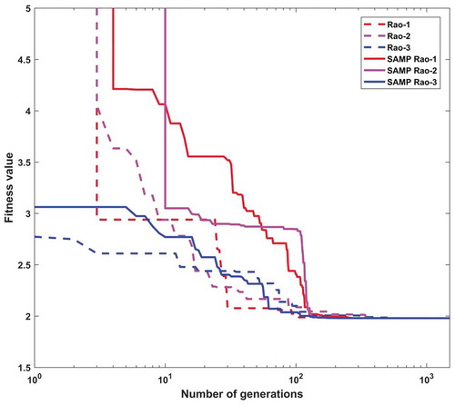
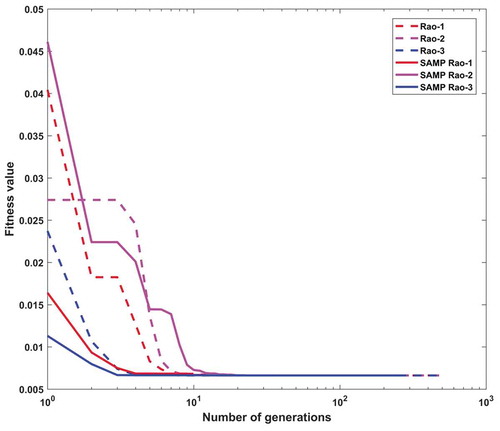
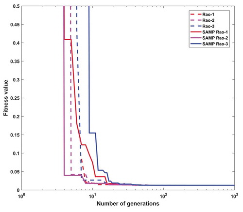
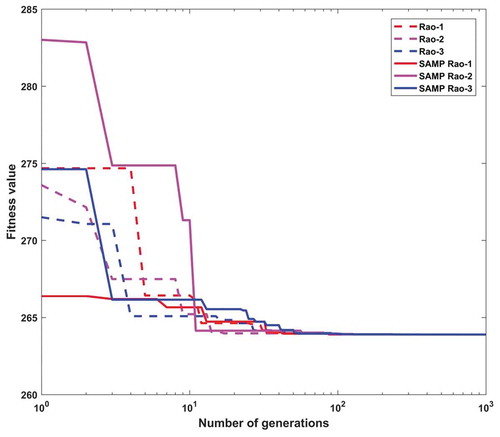
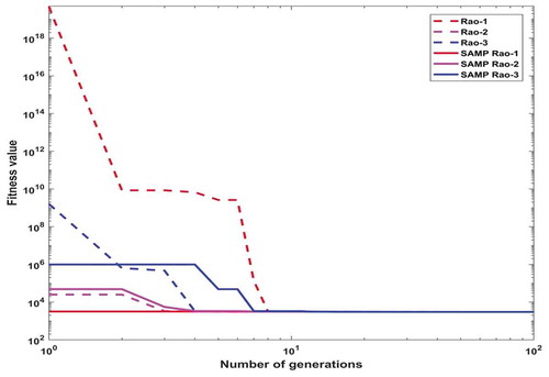
In this design problem, the population size and the maximum number of function evaluations are considered as 10 and 15,000, respectively, in each Rao and SAMP-Rao algorithm. Table 4 exhibits the optimal designs obtained for this problem using Rao and SAMP-Rao algorithms which are nearly the same, but SAMP-Rao algorithms have required less function evaluations than Rao algorithms to get the optimum solution for this problem. Table 5 presents the statistical results obtained using various optimization algorithms for the belleville spring problem over 50 runs. As shown in Table 5, the best fitness values obtained by Rao and SAMP-Rao algorithms are better than the other algorithms. Also, the best mean fitness value obtained using SAMP-Rao-1 algorithm is better than other algorithms. The standard deviation of results obtained by SAMP-Rao-1 algorithm is better than the other optimization algorithms considered for this problem. Figure 4 illustrates the speed of convergence of Rao and SAMP-Rao algorithms to reach the optimal solution of this problem. For this problem, the convergence speed of SAMP-Rao-3 algorithm is better and it has converged first to the optimum solution at 145th generation.

Table 4. Optimal designs of a belleville spring.

	Algorithm
Design variables	Rao-1	Rao-2	Rao-3	SAMP Rao-1	SAMP Rao-2	SAMP Rao-3
fmin	1.979674	1.979674	1.979674	1.979674	1.979674	1.979674
Do	12.01	12.01	12.01	12.01	12.01	12.01
Di	10.030473	10.030473	10.030473	10.030473	10.030473	10.030473
t	0.204143	0.204143	0.204143	0.204143	0.204143	0.204143
h	0.2	0.2	0.2	0.2	0.2	0.2
FEs	14,465	13,861	13,604	14,322	13,506	13,280
NP	10	10	10	10	10	10

Table 5. Comparison of statistical results of a belleville spring problem obtained over 50 runs.

Algorithm	Best	Mean	Worst	SD	maxFEs
WAO*	2.036250	2.233924	2.966195	1.5003E-01	15000
SSA*	1.979677	2.084371	2.361004	1.0203E-02	15000
MBA*	1.979675	1.979893	1.981627	3.6576E-04	15000
WCA*	1.979692	2.001388	2.164943	3.3176E-02	15000
GWO*	1.989215	2.009633	2.046591	1.4209E-02	15000
ER-WCA*	1.979698	2.009130	2.139935	3.2146E-02	15000
ALO*	1.983576	2.104509	2.368557	9.4178E-02	15000
MFO*	1.981209	2.062404	2.276791	6.4371E-02	15000
PSO*	1.979695	2.013715	2.350003	9.0931E-02	15000
ABC*	2.033455	2.167697	2.402849	7.5329E-02	15000
Rao-1	1.979674	1.979677	1.979704	5.5757E-06	15000
Rao-2	1.979674	2.004610	2.849536	1.3266E-01	15000
Rao-3	1.979674	2.021976	2.849536	1.7846E-01	15000
SAMP Rao-1	1.979674	1.979676	1.979683	1.7264E-06	15000
SAMP Rao-2	1.979674	1.983529	2.167558	2.6560E-02	15000
SAMP Rao-3	1.979674	1.979706	1.980113	7.7338E-05	15000

* The results of these algorithms are taken from Yildiz, Abderazek, and Mirjalili (2019).

Figure 4. Convergence plot for the belleville spring problem.

The objective of this problem is the minimization of the weight of a car while maintaining its safety rating score. This problem is taken from Yildiz, Abderazek, and Mirjalili (2019) and was formulated by Gu et al. (2001) using the European Enhanced Vehicle-safety Committees’ (EEVC) side-impact safety regulations. The total weight of some parts of the car, in which the gauges are defined as the design variables, is considered as an objective function (given as Problem 2 in Appendix B). This problem consists of 11 mixed-type design variables x₁–x₁₁. The variables x₁–x₇ are continuous variables related to the thicknesses of considered parts of the car, the variables x₈ and x₉ are discrete variables related to the material choice (i.e., either mild steel or high strength steel), and the variables x₁₀ and x₁₁ are continuous variables related to the noise factors. There are ten non-linear design constraints that are to be satisfied while reducing weight.

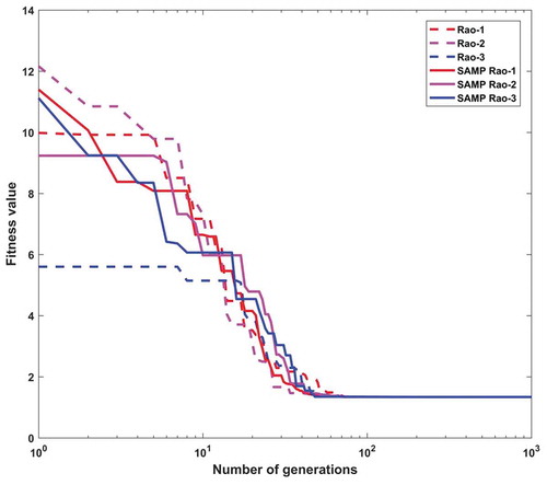
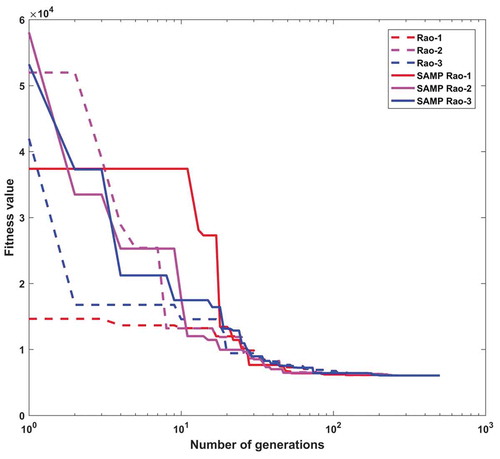
In this design problem, the population size and the maximum number of function evaluations are considered as 10 and 29,750, respectively, in each Rao and SAMP-Rao algorithm. Table 6 exhibits the optimal designs obtained for this problem using Rao algorithms and SAMP-Rao algorithms. The SAMP-Rao-2 algorithm obtained the best optimum design for this problem. Also, SAMP-Rao algorithms have required less function evaluations than Rao algorithms to get an optimum solution for this problem. Table 7 presents the statistical results obtained using various optimization algorithms for a car side impact problem over 50 runs. As shown in Table 7, the best fitness value obtained by SAMP-Rao-2 algorithm is better than the other algorithms. Also, the best mean fitness value obtained using SAMP-Rao-1 algorithm is better than the other algorithms. The standard deviation of results obtained by Rao-1 algorithm is better than other algorithms. Figure 5 illustrates the speed of convergence of Rao and SAMP-Rao algorithms to reach the optimal solution of this problem. For this problem, the convergence speed of SAMP-Rao-1 algorithm is better and it has converged first to optimum solution at the 160th generation.

Table 6. Optimal designs of a car side impact problem.

Design variables	Algorithm
	Rao-1	Rao-2	Rao-3	SAMP Rao-1	SAMP Rao-2	SAMP Rao-3
fmin	22.842934	22.842962	22.842952	22.842778	22.842474	22.842889
x1	0.5	0.5	0.5	0.5	0.5	0.5
x2	1.115454	1.115108	1.114729	1.117111	1.116409	1.112456
x3	0.5	0.5	0.5	0.5	0.5	0.5
x4	1.303705	1.304288	1.304915	1.300910	1.301776	1.308680
x5	0.5	0.5	0.5	0.5	0.5	0.5
x6	1.5	1.499987	1.5	1.5	1.500000	1.5
x7	0.5	0.5	0.5	0.5	0.500325	0.5
x8	0.345	0.345	0.345	0.345	0.345	0.345
x9	0.345	0.345	0.345	0.192	0.192	0.345
x10	−19.725672	−19.795653	−19.899042	−19.429599	−19.561806	−20.414686
x11	−0.313595	−0.079566	−0.401448	−0.187136	0.026451	−0.294756
FEs	25,640	28,600	25,000	23,794	22,636	22,390
NP	40	40	40	40	40	40

Table 7. Comparison of statistical results of a car side impact problem obtained over 50 runs.

Algorithm	Best	Mean	Worst	SD	maxFEs
WAO*	23.042162	24.814486	27.360813	9.6570E-01	29750
SSA*	22.846514	23.253716	23.829530	3.0557E-01	29750
MBA*	22.843596	22.936421	23.488942	1.5258E-01	29750
WCA*	22.843036	22.975164	23.370933	1.9772E-01	29750
GWO*	22.852792	22.992226	23.347095	1.6277E-01	29750
ER-WCA*	22.843264	23.069925	24.455312	3.5021E-01	29750
ALO*	22.842980	23.108402	23.824366	2.9093E-01	29750
MFO*	22.842970	22.972834	23.687547	2.0794E-01	29750
PSO*	22.842984	23.613571	26.190640	7.5252E-01	29750
ABC*	23.175889	23.860680	25.010762	3.7642E-01	29750
Rao-1	22.842934	22.888091	23.233663	1.1932E-01	29750
Rao-2	22.842962	22.899998	23.510730	1.5420E-01	29750
Rao-3	22.842952	22.932165	23.358370	1.4679E-01	29750
SAMP Rao-1	22.842778	22.846850	23.049444	2.9249E-02	29750
SAMP Rao-2	22.842474	22.887000	23.808878	1.5257E-01	29750
SAMP Rao-3	22.842889	22.880904	23.246891	8.9250E-02	29750

* The results of these algorithms are taken from Yildiz, Abderazek, and Mirjalili (2019).

Figure 5. Convergence plot for the car side impact problem.

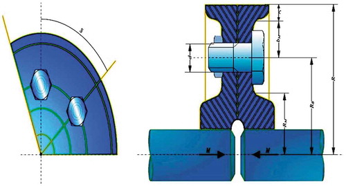
Figure 6 shows the schematic diagram of a coupling with a bolted rim. This problem is taken from Yildiz, Abderazek, and Mirjalili (2019). The N number of bolts placed at R_B radius having diameter d transmit a torque M by adhesion. The objective of this problem is the minimization of the radius of coupling, the torque, and the number of bolts simultaneously while satisfying eleven inequality design constraints (given as Problem 3 in Appendix B). This problem is a multi-objective problem with weighing coefficients of individual objectives as β₁, β₂, and β₃. There are four mixed-type design variables, such as the bolt diameter as d which is a discrete variable, the number of bolts as N which is an integer variable, the location of bolts from center of coupling as R_B and the torque transmitted as M which are continuous variables.

Figure 6. Schematic diagram of a coupling with a bolted rim (Yildiz, Abderazek, and Mirjalili 2019).

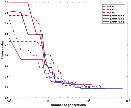
In this design problem, the population size and the maximum number of function evaluations are considered as 20 and 5,000, respectively, in each Rao and SAMP-Rao algorithm. Table 8 exhibits the optimal designs obtained for this problem using Rao algorithms and SAMP-Rao algorithms which are the same, but SAMP-Rao algorithms have required less function evaluations than Rao algorithms to get the optimum solution for this problem. Table 9 presents the statistical results obtained using various optimization algorithms for coupling with a bolted rim problem over 50 runs. As shown in Table 9, the best fitness value obtained by Rao and SAMP-Rao algorithm is better than the other algorithms. Also, the best mean fitness value obtained using SAMP-Rao-1 algorithm is better than the other algorithms. The standard deviation of results obtained by Rao-3 algorithm is better than the other algorithms. Figure 7 illustrates the speed of convergence of Rao and SAMP-Rao algorithms to reach the optimal solution of this problem. For this problem, the convergence speed of SAMP-Rao-3 algorithm is better and it has converged first to optimum solution at 10th generation.

Table 8. Optimal designs of a coupling with a bolted rim.

Design variables	Algorithm
	Rao-1	Rao-2	Rao-3	SAMP Rao-1	SAMP Rao-2	SAMP Rao-3
fmin	3.4	3.4	3.4	3.4	3.4	3.4
d	6	6	6	6	6	6
N	8	8	8	8	8	8
Rb	57.5	57.5	57.5	57.5	57.5	57.5
M	40	40	40	40	40	40
FEs	3,118	3,443	3,339	3,004	3,201	2,912
NP	20	20	20	20	20	20

Table 9. Comparison of statistical results of a coupling with a bolted rim problem obtained over 50 runs.

Algorithm	Best	Mean	Worst	SD	maxFEs
WAO*	3.480000	3.482102	3.552623	1.0670E-02	5000
SSA*	3.480000	3.480000	3.480000	1.6555E-08	5000
MBA*	3.480000	3.480000	3.480000	7.4154E-08	5000
WCA*	3.480000	3.480000	3.480000	1.1405E-09	5000
GWO*	3.480000	3.480188	3.480645	1.5178E-04	5000
ER-WCA*	3.480000	3.480000	3.480000	8.8909E-10	5000
ALO*	3.480000	3.480000	3.480000	9.5005E-09	5000
MFO*	3.480000	3.479999	3.480000	1.6943E-15	5000
PSO*	3.480000	3.539601	4.600000	2.1333E-01	5000
ABC*	3.480000	3.480001	3.480041	5.8746E-06	5000
Rao-1	3.400000	3.400000	3.400000	3.1402E-15	5000
Rao-2	3.400000	3.400000	3.400000	3.1402E-15	5000
Rao-3	3.400000	3.400000	3.400000	3.1402E-15	5000
SAMP Rao-1	3.400000	3.400000	3.400000	3.0073E-15	5000
SAMP Rao-2	3.400000	3.400000	3.400000	2.9723E-15	5000
SAMP Rao-3	3.400000	3.400000	3.400000	2.9641E-15	5000

* The results of these algorithms are taken from Yildiz, Abderazek, and Mirjalili (2019).

Figure 7. Convergence plot for the coupling with a bolted rim problem.

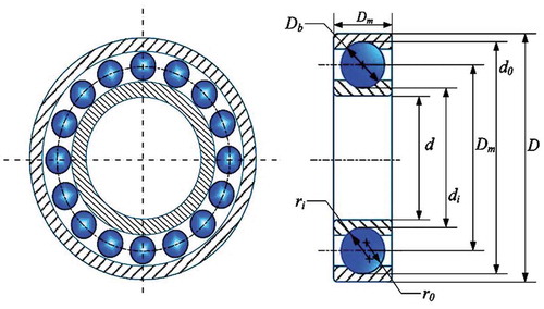
Figure 8 shows the schematic diagram of a rolling element bearing. This problem is taken from Yildiz, Abderazek, and Mirjalili (2019). The maximization of the dynamic load capacity of the rolling element bearing is the objective of this problem while satisfying nine non-linear inequality design constraints (given as Problem 4 in Appendix B). This problem consists of 10 variables out of which five are design variables, namely the pitch diameter of bearing as D_m, the diameter of balls as D_b, the number of balls as Z, the curvature coefficient of inner and outer raceway as f_i and f_o, and five variables are constraint parameters such as K_Dmin, K_Dmax, β, ε, and e. The number of balls Z is an integer variable and the remaining nine variables are continuous. The previous researchers had converted this problem into a minimization problem by multiplying the objective function by −1. Hence, in this paper also the objective function as presented by the previous researchers is considered.

Figure 8. Schematic diagram of a rolling element bearing (Yildiz, Abderazek, and Mirjalili 2019).

In the case of a rolling element bearing design problem, the population size and the maximum number of function evaluations are considered as 20 and 25,000, respectively, in each Rao and SAMP-Rao algorithm. Table 10 exhibits the optimal designs obtained for this problem using Rao and SAMP-Rao algorithms. The optimal designs obtained by Rao algorithms are nearly same as shown in Table 10, but SAMP-Rao algorithms have required less function evaluations than Rao algorithms to get the optimum solution for this problem. Table 11 shows statistical results obtained using different optimization algorithms for a rolling element bearing problem over 50 runs. The negative sign has occurred due to the conversion of the maximization problem to minimization problem. The results of other algorithms shown in Table 11 are found incorrect when the values of optimal design variables given by the authors are substituted in the objective function. The actual values of the fitness functions corresponding to the given best design variables are shown in Table 11 as the corrected best values. This might have happened due to consideration of incorrect formulations by the previous researchers. Hence, the results of these considered algorithms are required to be obtained again with correct formulations.

Table 10. Optimal designs of a rolling element bearing.

Design variables	Algorithm
	Rao-1	Rao-2	Rao-3	SAMP Rao-1	SAMP Rao-2	SAMP Rao-3
fmin	−81859.741597	−81859.741597	−81859.741597	−81859.741597	−81859.741597	−81859.741597
Dm	125.719056	125.719056	125.719056	125.719056	125.719056	125.719056
Db	21.425590	21.425590	21.425590	21.425590	21.425590	21.425590
Z	11	11	11	11	11	11
fi	0.515	0.515	0.515	0.515	0.515	0.515
fo	0.515	0.515	0.515	0.515	0.515	0.515
KDmin	0.487144	0.5	0.425908	0.400000	0.499999	0.499975
KDmax	0.613365	0.7	0.698588	0.681588	0.614931	0.639602
ε	0.3	0.3	0.3	0.3	0.3	0.3
e	0.098218	0.099999	0.025928	0.020000	0.020015	0.083386
β	0.846550	0.810140	0.85	0.782642	0.845021	0.831343
FEs	6880	6075	4535	6094	4272	4414
NP	20	20	20	20	20	20

Table 11. Comparison of statistical results of a rolling element bearing problem obtained over 50 runs.

Algorithm	Best	Corrected best	Mean	Worst	SD	maxFEs
WAO*	−85,433.018335	−81,743.340214	−69,384.18	−42,011.53	1.9229E+04	25,000
SSA*	−85,546.410556	−81,837.070844	−83,930.609521	−74,121.960572	2.8890E+03	25,000
MBA*	−85,546.801668	−81,857.250907	−85,545.918790	−85,528.981256	3.9311E+00	25,000
WCA*	−85,546.801669	−81,857.250907	−85,320.986197	−80,482.382194	8.4006E+02	25,000
GWO*	−85,529.083044	−77,633.397960	−83,395.084960	−43,543.450846	8.2245E+03	25,000
ER-WCA*	−85,546.801668	−81,857.250907	−85,198.285411	−80,481.640316	1.2258E+03	25,000
ALO*	−85,546.637712	−81,648.595595	−84,032.863623	−73,872.816454	3.1218E+03	25,000
MFO*	−85,546.801669	−81,857.250907	−85,459.048355	−84,459.784937	2.9768E+02	25,000
PSO*	−85,546.805166	−81,857.250907	−81,775.478308	−33,705.060621	8.1802E+03	25,000
ABC*	−85,428.249543	−81,741.794843	−85,121.754420	−83,859.085138	3.6257E+02	25,000
Rao-1	-	−81,859.741597	−81,859.741597	−81,859.741597	1.0290E-10	25,000
Rao-2	-	−81,859.741597	−81,606.710464	−73,415.731009	1.2166E+03	25,000
Rao-3	-	−81,859.741597	−80,910.151887	−73,415.731009	2.5433E+03	25,000
SAMP Rao-1	-	−81,859.741597	−81,859.741597	−81859.741597	9.7018E-11	25,000
SAMP Rao-2	-	−81,859.741597	−81,754.552945	−80,807.855077	3.1877E+02	25,000
SAMP Rao-3	-	−81,859.741597	−81,500.943443	−73,415.731009	1.6738E+03	25,000

* The results of these algorithms are taken from Yildiz, Abderazek, and Mirjalili (2019).

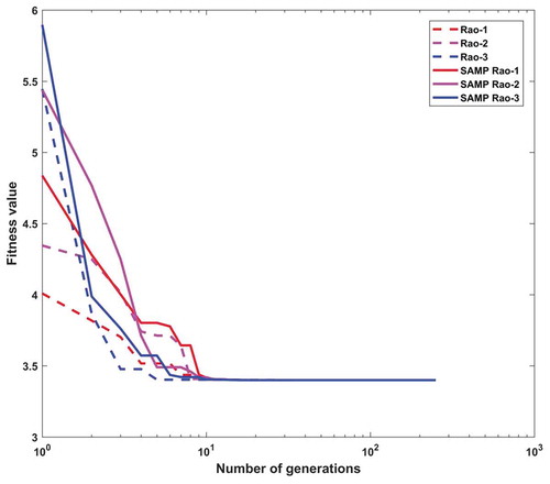
Table 11 shows statistical results obtained using different optimization algorithms for a rolling element bearing problem over 50 runs. As shown in Table 11, the best fitness values obtained by Rao and SAMP-Rao algorithms are better than the other algorithms. Also, the best mean fitness value obtained using the SAMP-Rao-1 algorithm is the same as Rao-1 algorithm and better than the other algorithms. The standard deviation of results obtained by SAMP-Rao-1 algorithm is better than the other optimization algorithms considered for this problem. Figure 9 illustrates the speed of convergence of Rao and SAMP-Rao algorithms to reach the optimal solution of this problem. For this problem, the convergence speed of SAMP-Rao-2 algorithm is better and it has converged first to optimum solution at 64th generation.

Figure 9. Convergence plot for the rolling element bearing problem.

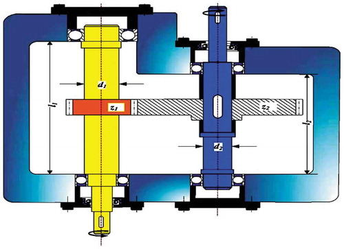
Figure 10 shows the schematic diagram of a speed reducer. This problem is taken from Yildiz, Abderazek, and Mirjalili (2019). The minimization of its total weight is the objective of this design problem (given as Problem 5 in Appendix B). There are seven design variables, namely, the face width as b, the module of teeth as m, the number of teeth on pinion as Z, the length of shaft 1 between bearings as l₁, the length of shaft 2 between bearings as l₂, shaft 1 diameter as d₁, and the shaft 2 diameter as d₂. All are continuous-type design variables except Z which is an integer design variable. This problem is having eleven constraints which are related to the bending stress in the gear teeth, the surface stress, the stresses in the two shafts, and transverse deflections of the two shafts due to transmitted load.

Figure 10. Schematic diagram of a speed reducer (Yildiz, Abderazek, and Mirjalili 2019).

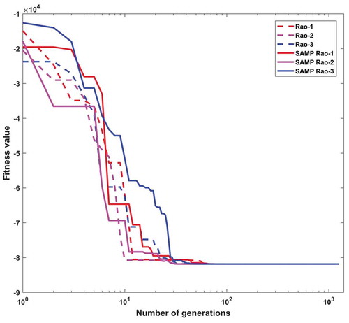
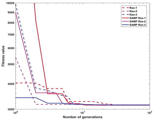
In the case of a speed reducer design problem, the maximum number of function evaluations and the number of populations are considered as 25,000 and 10, respectively, in each Rao and SAMP-Rao algorithm. Table 12 exhibits the optimal designs obtained for this problem using Rao and SAMP-Rao algorithms. The optimal designs obtained by Rao algorithms and SAMP-Rao are nearly the same as shown in Table 12, but SAMP-Rao algorithms have required less function evaluations than Rao algorithms to get the optimum solution for this problem. Table 13 shows statistical results obtained using different optimization algorithms for a speed reducer problem over 50 runs. As shown in Table 13, the best fitness values obtained by Rao and SAMP-Rao algorithms are better than the other algorithms. Also, the best mean fitness values obtained using SAMP-Rao algorithms are the same as Rao-1 algorithm and better than the other algorithms. The standard deviation of results obtained by SAMP-Rao-1 algorithm is better than the other optimization algorithms considered for this problem. Figure 11 illustrates the speed of convergence of Rao and SAMP-Rao algorithms to reach the optimal solution of this problem. For this problem, the convergence speed of SAMP-Rao-3 algorithm is better and it has converged first to optimum solution at 67th generation.

Table 12. Optimal designs of a speed reducer.

Design variables	Algorithm
	Rao-1	Rao-2	Rao-3	SAMPRao-1	SAMPRao-2	SAMPRao-3
fmin	2,994.345132	2,994.345132	2,994.345132	2,994.345132	2,994.345132	2,994.345132
b	3.5	3.5	3.5	3.5	3.5	3.5
m	0.7	0.7	0.7	0.7	0.7	0.7
Z	17	17	17	17	17	17
l1	7.3	7.3	7.3	7.3	7.3	7.3
l2	7.715320	7.715320	7.715320	7.715320	7.715320	7.715320
d1	3.350215	3.350215	3.350215	3.350215	3.350215	3.350215
d2	5.286654	5.286654	5.286654	5.286654	5.286654	5.286654
FEs	24,714	24,461	24,183	22,511	23,380	23,385
NP	40	40	40	40	40	40

Table 13. Comparison of statistical results of a speed reducer problem obtained over 50 runs.

Algorithm	Best	Mean	Worst	SD	maxFEs
WAO*	2,996.604340	3,042.915000	3,233.598124	4.0888E+01	25,000
SSA*	2,996.021720	3,005.574377	3,015.662612	4.6387E+00	25,000
MBA*	2,994.471371	2,994.744437	2,994.484788	2.4195E-03	25,000
WCA*	2,994.471066	2,996.203773	3,016.578575	4.8705E+00	25,000
GWO*	2,995.704434	3,001.556162	3,009.944296	4.1218E+00	25,000
ER-WCA*	2,994.471066	2,996.744541	3,007.436552	4.3876E+00	25,000
ALO*	2,996.521745	3,005.644279	3,014.379001	4.7422E+00	25,000
MFO*	2,994.471066	2,994.471000	2,994.471000	7.3921E-10	25,000
PSO*	2,994.471069	3,070.655058	3,209.297397	5.8657E+01	25,000
ABC*	2,994.471067	2,994.471075	2,994.471115	9.2123E-06	25,000
Rao-1	2,994.345132	2,994.345132	2,994.345132	1.8443E-12	25,000
Rao-2	2,994.345132	2,995.916235	3,033.622701	7.7749E+00	25,000
Rao-3	2,994.345132	2,996.701786	3,033.622701	9.4226E+00	25,000
SAMP Rao-1	2,994.345132	2,994.345132	2,994.345132	1.9489E-13	25,000
SAMP Rao-2	2,994.345132	2,994.345132	2,994.345132	7.6429E-12	25,000
SAMP Rao-3	2,994.345132	2,994.345132	2,994.345132	3.2959E-12	25,000

* The results of these algorithms are taken from Yildiz, Abderazek, and Mirjalili (2019).

Figure 11. Convergence plot for the speed reducer problem.

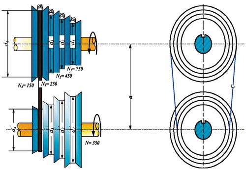
Figure 12 shows the schematic diagram of a step-cone pulley. This problem is taken from Yildiz, Abderazek, and Mirjalili (2019). The minimization of its weight is the objective of this design problem (given as Problem 6 in Appendix B). There are five design variables with step diameters as d₁, d₂, d₃, and d₄, respectively, and the pulley width w. This problem is having eleven design constraints in which three are equality constraints and eight are inequality constraints. The power transmitted by this pulley is to be at least 0.75 HP with 350 rpm input speed, and output speeds at each step are 750, 450, 250, and 150 rpm, respectively.

Figure 12. Schematic diagram of a step-cone pulley (Yildiz, Abderazek, and Mirjalili 2019).

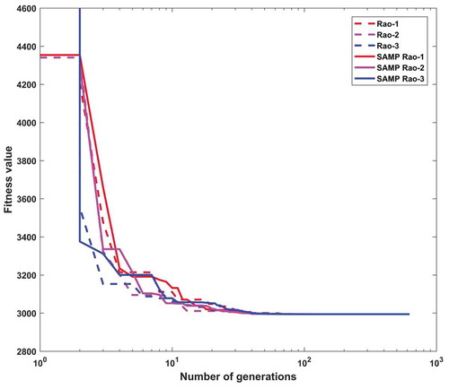
In the case of a step-cone pulley design problem, the maximum number of function evaluations and the number of populations are considered as 15,000 and 10, respectively, in each Rao and SAMP-Rao algorithm. Table 14 exhibits the optimal designs obtained for this problem using Rao and SAMP-Rao algorithms. The optimal designs obtained by Rao and SAMP-Rao algorithms are exactly the same as shown in Table 14. Table 15 shows statistical results obtained using different optimization algorithms for a step-cone pulley problem over 50 runs. As shown in Table 15, the best fitness values obtained by Rao and SAMP-Rao algorithms are the same as SSA and MFO algorithms, and better than other algorithms. Also, the best mean fitness value obtained using the SAMP-Rao-1 algorithm is better than the other algorithms. The standard deviation of results obtained by SAMP-Rao-1 algorithm is better than the other optimization algorithms considered for this problem. Figure 13 illustrates the speed of convergence of Rao and SAMP-Rao algorithms to reach the optimal solution of this problem. For this problem, the convergence speed of SAMP-Rao-2 algorithm is better and it has converged first to optimum solution at 30th generation.

Table 14. Optimal designs of a step-cone pulley.

Design variables	Algorithm
	Rao-1	Rao-2	Rao-3	SAMP Rao-1	SAMP Rao-2	SAMP Rao-3
fmin	16.634504	16.634504	16.634504	16.634504	16.634504	16.634504
d1	40	40	40	40	40	40
d2	54.764301	54.764301	54.764301	54.764301	54.764301	54.764301
d3	73.013177	73.013177	73.013177	73.013177	73.013177	73.013177
d4	88.428420	88.428420	88.428420	88.428420	88.428420	88.428420
w	85.986243	85.986243	85.986243	85.986243	85.986243	85.986243
FEs	8589	6903	6312	9471	7974	8745
NP	10	10	10	10	10	10

Table 15. Comparison of statistical results of a step-cone pulley problem obtained over 50 runs.

Algorithm	Best	Mean	Worst	SD	maxFEs
WAO*	16.634521	20.938294	24.848825	3.3498E+00	15000
SSA*	16.634504	17.286354	19.045457	1.8164E-01	15000
MBA*	16.634507	16.702535	18.323714	2.6279E-01	15000
WCA*	16.634508	17.530376	18.833029	9.2296E-01	15000
GWO*	16.647961	18.128588	19.015492	9.3755E-01	15000
ER-WCA*	16.634509	17.647333	18.832978	8.3766E-01	15000
ALO*	16.634508	16.789416	18.015810	3.6058E-01	15000
MFO*	16.634504	17.839171	24.777860	1.4201E+00	15000
PSO*	16.634521	20.938294	24.848825	3.3498E+00	15000
ABC*	16.648275	16.791388	17.468562	1.8164E-01	15000
Rao-1	16.634504	17.058070	19.354135	7.0999E-01	15000
Rao-2	16.634504	17.532656	19.379791	1.1492E+00	15000
Rao-3	16.634504	17.247839	19.387243	9.0818E-01	15000
SAMP Rao-1	16.634504	16.696366	17.115707	1.1316E-01	15000
SAMP Rao-2	16.634504	17.449175	19.240789	9.3855E-01	15000
SAMP Rao-3	16.634504	17.115218	19.240789	9.1497E-01	15000

* The results of these algorithms are taken from Yildiz, Abderazek, and Mirjalili (2019).

Figure 13. Convergence plot for the step-cone pulley problem.

Figure 14 shows the schematic diagram of a welded beam. This problem is taken from Hashim et al. (2019). The objective of this design problem is the minimization of fabrication cost (given as Problem 7 in Appendix B). There are four design variables, i.e., the thickness of weld as h(x₁), the length of an attached part of the bar as l(x₂), the height of the bar as t(x₃) and the thickness of the bar as b(x₄₎. This design problem is having seven constraint equations which are related to the bending stress in the beam (σ), the end deflection of the beam (δ), the shear stress (τ), the bucking load on the beam (P_c), and the side constraints.

Figure 14. Schematic diagram of a welded beam.

In the welded beam problem, the maximum number of function evaluations and the number of populations are considered as 5,000 and 10, respectively, in each Rao and SAMP-Rao algorithm. In this problem, the optimum designs obtained by Rao and SAMP-Rao algorithms are nearly equal as shown in Table 17, but SAMP-Rao algorithms have required less function evaluations than Rao algorithms to get the optimum solution for this problem. From Table 16, the solution given by MFO, i.e., 1.72452 is nearest to the solution given by Rao and SAMP-Rao algorithms for this problem. But the solution given by MFO is an infeasible solution due to violation of two constraints. So, the optimal solution given by Rao and SAMP-Rao algorithms for this problem is superior to GWO, ALO, MVO, MFO, WOA, and HGSO algorithms.

Table 16. Comparison of best fitness values of different optimization algorithms for the seven engineering design problems considered.

Algorithm	Welded beam	I-beam	Cantilever beam	Tension/Compression Spring	Pressure vessel	Gear train	3-bar truss
CS*	NA	0.0130747	1.33999	NA	6059.7143348	2.701e-12	263.9716
GWO*	1.72624	NA	NA	0.012666	6051.5639^c	NA	NA
ALO*	NA	NA	1.33995	NA	NA	2.7009e-12	263.895843
MFO*	1.72452^a	0.0066259	1.339988	NA	6059.7143	2.7009e-12	263.895979
MVO*	1.72645	NA	1.339959	NA	6060.8066	2.7009e-12	263.895849
WOA*	1.730499	NA	NA	0.0126763	6059.7410	NA	NA
HGSO*	1.7260	NA	NA	0.01265^b	NA	NA	NA
Rao-1	1.724852	0.0066259	1.339958	0.012666	6059.714334	2.7009e-12	263.895841
Rao-2	1.724852	0.0066259	1.339957	0.012669	6059.714334	2.7009e-12	263.895845
Rao-3	1.724852	0.0066259	1.339957	0.012672	6059.714334	2.7009e-12	263.895843
SAMP Rao-1	1.724852	0.0066259	1.339957	0.012666	6059.714334	2.7009e-12	263.895837
SAMP Rao-2	1.724852	0.0066259	1.339957	0.012667	6059.714334	2.7009e-12	263.895842
SAMP Rao-3	1.724852	0.0066259	1.339957	0.012669	6059.714334	2.7009e-12	263.895826

*CS (Gandomi, Yang, and Alavi 2013); GWO (Mirjalili, Mirjalili, and Lewis 2014); ALO (Mirjalili 2015b); MFO (Mirjalili 2015a); MVO (Mirjalili and Lewis 2016); WOA (Mirjalili and Lewis 2016); HGSO (Hashim et al. 2019).

^aAn infeasible solution due to violation of two constraints.

^bAn infeasible solution due to violation of one constraint.

^cAn infeasible solution because of variable T_h (x₂) is not an integer multiple of 0.0625 in. (i.e., 0.4345/0.0625 = 6.952)

Table 17. Optimal designs of a welded beam.

Design variables	Algorithm
	Rao-1	Rao-2	Rao-3	SAMP Rao-1	SAMP Rao-2	SAMP Rao-3
fmin	1.724852	1.724852	1.724852	1.724852	1.724852	1.724852
h	0.205730	0.205730	0.205730	0.205730	0.205730	0.205730
l	3.470487	3.470487	3.470488	3.470489	3.470489	3.470489
t	9.036624	9.036624	9.036624	9.036624	9.036624	9.036624
b	0.205730	0.205730	0.205730	0.205730	0.205730	0.205730
FEs	4790	4768	4831	4638	4626	4714
NP	10	10	10	10	10	10

Table 18 shows statistical results obtained using Rao and SAMP-Rao algorithms for this problem over 50 runs. As shown in Table 18, the best and best mean fitness values obtained by Rao and SAMP-Rao algorithms are the same, but the standard deviation of results obtained by the SAMP-Rao-1 algorithm is better than the other algorithms. Figure 15 illustrates the speed of convergence of Rao and SAMP-Rao algorithms to reach the optimal solution of this problem. For this problem, the convergence speed of the SAMP-Rao-2 algorithm is better and it has converged first to optimum solution at 170th generation.

Table 18. Statistical results of a welded beam problem obtained over 50 runs.

Algorithm	Best	Mean	Worst	SD	maxFEs
Rao-1	1.724852	1.724852	1.724852	1.1387E-08	5000
Rao-2	1.724852	1.724852	1.724852	1.0219E-08	5000
Rao-3	1.724852	1.724852	1.724852	5.1434E-08	5000
SAMP Rao-1	1.724852	1.724852	1.724852	1.0017E-08	5000
SAMP Rao-2	1.724852	1.724852	1.724852	3.4096E-08	5000
SAMP Rao-3	1.724852	1.724852	1.724852	5.2798E-08	5000

Figure 15. Convergence plot for the welded beam problem.

Figure 16 shows the schematic diagram of an I-beam. This problem is taken from Mirjalili (2015a). The objective of this design problem is the minimization of its vertical deflection (given as Problem 8 in Appendix B). There are four design variables as cross-sectional dimensions of I-beam, i.e., the overall width as b (x₁), the overall height as h (x₂), the thickness of the web as t_w (x₃) and the thickness of flange as t_h (x₄). The constraint equation in this problem is related to the cross-sectional area of an I-beam.

Figure 16. Schematic diagram of an I-beam.

In the I-beam problem, the maximum number of function evaluations and the number of populations are considered as 5000 and 10, respectively, in each Rao and SAMP-Rao algorithm. In this problem, the optimum designs obtained by Rao and SAMP-Rao algorithms are the same as shown in Table 19, but SAMP-Rao algorithms have required less function evaluations than Rao algorithms to get the optimum solution for this problem. From Table 16, the optimal solution given by Rao and SAMP-Rao algorithms is the same as the solution given by MFO algorithm and superior to CS algorithm for an I-beam problem. Table 20 shows statistical results obtained using Rao and SAMP-Rao algorithms for this problem over 50 runs. As shown in Table 20, the best mean fitness values and the standard deviation of results obtained by SAMP-Rao algorithms are better than the Rao algorithms. Figure 17 illustrates the speed of convergence of Rao and SAMP-Rao algorithms to reach the optimal solution of this problem. For this problem, the convergence speed of the SAMP-Rao-3 algorithm is better and it has converged first to optimum solution at 23rd generation.

Table 19. Optimal designs of an I-beam.

Design variables	Algorithm
	Rao-1	Rao-2	Rao-3	SAMP Rao-1	SAMP Rao-2	SAMP Rao-3
fmin	0.0066259	0.0066259	0.0066259	0.0066259	0.0066259	0.0066259
b	50	50	50	50	50	50
h	80	80	80	80	80	80
tw	1.764705	1.764706	1.764706	1.764706	1.764706	1.764706
th	5	5	5	5	5	5
FEs	1,419	1,446	2,237	1,350	1,300	1,203
NP	10	10	10	20	20	20

Table 20. Statistical results of an I-beam problem obtained over 50 runs.

Algorithm	Best	Mean	Worst	SD	maxFEs
Rao-1	0.0066259	0.0066409	0.0068503	5.6925E-05	5000
Rao-2	0.0066259	0.0066634	0.0068503	8.5049E-05	5000
Rao-3	0.0066259	0.0066409	0.0068503	5.6925E-05	5000
SAMP Rao-1	0.0066259	0.0066259	0.0066259	1.7523E-18	5000
SAMP Rao-2	0.0066259	0.0066259	0.0066259	1.7523E-18	5000
SAMP Rao-3	0.0066259	0.0066259	0.0066259	1.7523E-18	5000

Figure 17. Convergence plot for the I-beam problem.

Figure 18 shows the schematic diagram of a cantilever beam. This problem is taken from Mirjalili and Mirjalili (2016). The objective of this design problem is the minimization of its weight (given as Problem 9 in Appendix B). This cantilever beam is having five elements which are hollow and square in cross-section. The thickness of the hollow cross-section of all five elements is constant. Also, a vertical load is applied at the free end of the beam and the other end is rigidly supported. The side length of the square cross-section of each element is a design parameter. So this problem has five design variables. The constraint equation in this problem is related to the vertical displacement of the beam.

Figure 18. Schematic diagram of a cantilever beam.

In the cantilever beam problem, the maximum number of function evaluations and the number of populations are considered as 10000 and 10, respectively, in each Rao and SAMP-Rao algorithm. In this problem, the optimum designs obtained by Rao and SAMP-Rao algorithms are nearly the same as shown in Table 21, but SAMP-Rao algorithms have required less function evaluations than Rao algorithms to get the optimum solution for this problem. As shown in Table 16, the optimal solutions given by SAMP-Rao algorithms for a cantilever beam design problem are superior to CS, MFO, and MVO algorithms and competitive with ALO algorithm. Table 22 shows statistical results obtained using Rao and SAMP-Rao algorithms for this problem over 50 runs. As shown in Table 22, the best mean fitness values and the standard deviation of results obtained by the SAMP-Rao-1 algorithm are better than the other algorithms. Figure 19 illustrates the speed of convergence of Rao and SAMP-Rao algorithms to reach the optimal solution of this problem. For this problem, the convergence speed of the SAMP-Rao-3 algorithm is better and it has converged first to optimum solution at the 48th generation.

Table 21. Optimal designs of a cantilever beam.

Design variables	Algorithm
	Rao-1	Rao-2	Rao-3	SAMP Rao-1	SAMP Rao-2	SAMP Rao-3
fmin	1.339958	1.339957	1.339957	1.339957	1.339957	1.339957
x1	6.010575	6.012820	6.017600	6.019652	6.015386	6.017337
x2	5.310288	5.309512	5.308477	5.307321	5.307974	5.311291
x3	4.496193	4.496385	4.492312	4.492792	4.495085	4.494742
x4	3.504149	3.503597	3.502903	3.501437	3.499924	3.499465
x5	2.152484	2.151360	2.152373	2.152471	2.155307	2.150834
FEs	8558	8617	8837	8420	8549	8605
NP	10	10	10	10	10	10

Table 22. Statistical results of a cantilever beam problem obtained over 50 runs.

Algorithm	Best	Mean	Worst	SD	maxFEs
Rao-1	1.339958	1.339968	1.339984	6.6086E-06	10000
Rao-2	1.339957	1.339966	1.339994	8.6796E-06	10000
Rao-3	1.339957	1.339966	1.339995	8.1907E-06	10000
SAMP Rao-1	1.339957	1.339965	1.339981	5.8948E-06	10000
SAMP Rao-2	1.339957	1.339966	1.339989	6.7825E-06	10000
SAMP Rao-3	1.339957	1.339966	1.339989	7.7507E-06	10000

Figure 19. Convergence plot for the cantilever beam problem.

Figure 20 shows the schematic diagram of a tension/compression spring. This problem is taken from Hashim et al. (2019). The objective of this design problem is the minimization of its weight (given as Problem 10 in Appendix B). As shown in Figure 20, this problem is having three design variables, namely, the wire diameter as d (x₁), the mean coil diameter as D (x₂) and the number of active coils as N (x₃). This problem is having four constraints which are related to the shear stress, the minimum deflection, the surge frequency, and limits on the outside diameter and on the design variables.

Figure 20. Schematic diagram of a tension/compression spring.

In the tension/compression spring problem, the maximum number of function evaluations and the number of populations are considered as 10,000 and 10, respectively, in each Rao and SAMP-Rao algorithm. In this problem, the optimum designs obtained by Rao-1 and SAMP-Rao-1 algorithms are the same and better than other the algorithms as shown in Table 23, but the SAMP-Rao-1 algorithm has required less function evaluations than Rao-1 algorithm to get the optimum solution for this problem. As shown in Table 16, the solution given by SAMP-Rao-1 is the same as the solution given by the GWO algorithm. Also, the solution given by the HGSO algorithm for this problem, i.e., 0.01265 is an infeasible solution due to violation of one constraint. The optimal solution given by the SAMP-Rao-1 algorithm for this problem is better than the WOA algorithm. Table 24 shows statistical results obtained using Rao and SAMP-Rao algorithms for this problem over 50 runs. As shown in Table 24, the best mean fitness values and the standard deviation of results obtained by the SAMP-Rao-1 algorithm are better than the other algorithms. Figure 21 illustrates the speed of convergence of Rao and SAMP-Rao algorithms to reach the optimal solution of this problem. For this problem, the convergence speed of the SAMP-Rao-2 algorithm is better and it has converged first to optimum solution at the 40th generation.

Table 23. Optimal designs of a tension/compression spring.

Design variables	Algorithm
	Rao-1	Rao-2	Rao-3	SAMP Rao-1	SAMP Rao-2	SAMP Rao-3
fmin	0.012666	0.012669	0.012672	0.012666	0.012667	0.012669
d	0.051654	0.051217	0.051445	0.051654	0.052020	0.051290
D	0.355859	0.345455	0.350813	0.355859	0.364719	0.347177
N	11.340849	11.981684	11.648891	11.340849	10.835314	11.871772
FEs	6,793	6,429	6,004	6,078	6,287	5,886
NP	10	10	10	10	10	10

Table 24. Statistical results of a tension/compression spring problem obtained over 50 runs.

Algorithm	Best	Mean	Worst	SD	maxFEs
Rao-1	0.012666	0.012712	0.012846	3.6195E-05	10,000
Rao-2	0.012669	0.013232	0.030455	2.5886E-03	10,000
Rao-3	0.012672	0.013086	0.017773	1.2062E-03	10,000
SAMP Rao-1	0.012666	0.012709	0.012818	3.5852E-05	10,000
SAMP Rao-2	0.012667	0.013246	0.017773	1.5264E-03	10,000
SAMP Rao-3	0.012669	0.013471	0.017773	1.7625E-03	10,000

Figure 21. Convergence plot for the tension/compression spring problem.

Figure 22 shows the schematic diagram of a pressure vessel. This problem is taken from Mirjalili and Mirjalili (2016). The objective of this design problem is the minimization of the total cost (given as Problem 11 in Appendix B). This total cost comprises the cost of the material, welding, and forming. As shown in Figure 22, this problem is having four design variables, namely, the thickness of the shell as T_s (x₁), the thickness of the head as T_h (x₂), the inner radius of the shell as R(x₃), and the length of the cylindrical section of the vessel without considering the head as L(x₄). The first two design variables, i.e., T_s and T_h must be integer multiples of 0.0625 in. due to the available thickness of rolled steel plates. Remaining two variables, i.e., R and L are continuous. This problem is having four design constraints.

Figure 22. Schematic diagram of a pressure vessel.

In the pressure vessel problem, the maximum number of function evaluations and the number of populations are considered as 10,000 and 20, respectively, in each Rao and SAMP-Rao algorithm. In this problem, the optimum designs obtained by Rao and SAMP-Rao algorithms are the same as shown in Table 25, but SAMP-Rao algorithms have required less function evaluations than Rao algorithms to get the optimum solution for this problem. In Table 16, the solution given by GWO algorithm for pressure vessel problem, i.e., 6,051.5639 is an infeasible solution because variable T_h (x₂) is not an integer multiple of 0.0625 in. (Mirjalili, Mirjalili, and Lewis 2014). As shown in Table 16, the optimal solution given by SAMP-Rao algorithms for this problem is nearest to the solutions given by CS and MFO algorithms, and superior to MVO and WOA algorithms. Table 26 shows statistical results obtained using Rao and SAMP-Rao algorithms for this problem over 50 runs. As shown in Table 26, the standard deviation of results obtained by Rao-2 algorithm is better than the other algorithms, but the best mean fitness value obtained by the SAMP-Rao-2 algorithm is better than the other algorithms. Figure 23 illustrates the speed of convergence of Rao and SAMP-Rao algorithms to reach the optimal solution of this problem. For this problem, the convergence speed of the SAMP-Rao-1 algorithm is better and it has converged first to optimum solution at the 120th generation.

Table 25. Optimal designs of a pressure vessel.

Design variables	Algorithm
	Rao-1	Rao-2	Rao-3	SAMP Rao-1	SAMP Rao-2	SAMP Rao-3
fmin	6059.714334	6059.714334	6059.714334	6059.714334	6059.714334	6059.714334
Ts	0.8125	0.8125	0.8125	0.8125	0.8125	0.8125
Th	0.4375	0.4375	0.4375	0.4375	0.4375	0.4375
R	42.098446	42.098446	42.098446	42.0984456	42.0984456	42.0984456
L	176.636596	176.636596	176.636596	176.636596	176.636596	176.636596
FEs	6,855	8,691	8,779	6,816	8,364	8,204
NP	20	20	20	20	20	20

Table 26. Statistical results of a pressure vessel problem obtained over 50 runs.

Algorithm	Best	Mean	Worst	SD	maxFEs
Rao-1	6059.714334	6069.230694	6093.903548	10.451664	10000
Rao-2	6059.714334	6062.055668	6090.526202	7.171409	10000
Rao-3	6059.714334	6061.883052	6090.526202	7.810982	10000
SAMP Rao-1	6059.714334	6068.004283	6093.713518	10.088323	10000
SAMP Rao-2	6059.714334	6061.786654	6370.779827	44.594750	10000
SAMP Rao-3	6059.714334	6061.821818	6370.779713	44.546246	10000

Figure 23. Convergence plot for the pressure vessel problem.

Figure 24 shows the schematic diagram of a gear train. This problem is taken from Mirjalili and Mirjalili (2016). The objective of this design problem is the minimization of the gear ratio (given as Problem 12 in Appendix B) . As shown in Figure 24, this problem is having four design variables as the number of teeth on four gears of a gear train, i.e., n_A (x₁), n_B (x₂), n_C (x₃), and n_D (x₄). All these four design variables must be integer variables. In addition to this, the problem is having a design constraint.

Figure 24. Schematic diagram of a gear train.

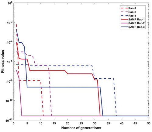
In the gear train problem, the maximum number of function evaluations and the number of populations are considered as 500 and 10, respectively, in each Rao and SAMP-Rao algorithm. In this problem, the values of design variables x₂ and x₃ as well as x₁ and x₄ are interchangeable due to its mathematical formulations. So that there are different combinations of design variables for the same value of optimal gear ratio. As shown in Table 27, even if the Rao and SAMP-Rao algorithms got different sets of optimal design variables, but their corresponding optimal values of fitness function, i.e., gear ratios are equal, i.e., 2.7009e-12. As shown in Table 16, the optimal fitness value given by SAMP-Rao algorithms is the same as other algorithms. Even though SAMP-Rao algorithms have required more function evaluations than Rao algorithms to get the optimum solution for this problem, the best mean fitness value and the standard deviation of results obtained by SAMP-Rao algorithms are better than the Rao algorithms as shown in Table 28. Figure 25 illustrates the speed of convergence of Rao and SAMP-Rao algorithms to reach the optimal solution of this problem. For this problem, the convergence speed of the SAMP-Rao-2 algorithm is better and it has converged first to optimum solution at the third generation.

Table 27. Optimal designs of a gear train.

Design variables	Algorithm
	Rao-1	Rao-2	Rao-3	SAMP Rao-1	SAMP Rao-2	SAMP Rao-3
fmin	2.7009E-12	2.7009E-12	2.7009E-12	2.7009E-12	2.7009E-12	2.7009E-12
nA	49	43	49	43	43	49
nB	16	16	19	19	19	16
nC	19	19	16	16	16	19
nD	43	49	43	49	49	43
FEs	108	235	108	210	279	270
NP	10	10	10	10	10	10

Table 28. Statistical results of a gear train problem obtained over 50 runs.

Algorithm	Best	Mean	Worst	SD	maxFEs
Rao-1	2.7009E-12	9.6288E-08	1.2045E-06	2.6504E-07	500
Rao-2	2.7009E-12	5.7864E-08	8.9490E-07	1.6169E-07	500
Rao-3	2.7009E-12	1.2022E-07	8.9490E-07	2.5475E-07	500
SAMP Rao-1	2.7009E-12	1.9898E-08	1.5244E-07	3.0089E-08	500
SAMP Rao-2	2.7009E-12	2.8413E-08	5.0415E-07	7.4334E-08	500
SAMP Rao-3	2.7009E-12	1.6216E-08	7.8022E-08	1.7207E-08	500

Figure 25. Convergence plot for the gear train problem.

The objective of a 3-bar truss design problem is the minimization of its total weight (given as Problem 13 in Appendix B). This problem is taken from Mirjalili and Mirjalili (2016). As shown in Figure 26, this problem is having two design variables, i.e., the areas of bar 1 and 3 as A₁ (x₁) and the area of bar 2 as A₂ (x₂). This problem is having three design constraints related to stress in each of the truss members.

Figure 26. Schematic diagram of a 3-bar truss.

In the 3-bar truss problem, the maximum number of function evaluations and the number of populations are considered as 10,000 and 10, respectively, in each Rao and SAMP-Rao algorithm. As shown in Table 16, the optimal fitness value given by the SAMP-Rao-3 algorithm is better than other algorithms. In this problem, the optimum designs obtained by SAMP-Rao algorithms are better than corresponding Rao algorithms as shown in Table 29. Also, SAMP-Rao algorithms have required less function evaluations than Rao algorithms to get an optimum solution for this problem. As shown in Table 30, the best mean fitness value obtained by the SAMP-Rao-2 algorithm is better than other algorithms and the standard deviation of results obtained by the SAMP-Rao-1 algorithm is better than the other algorithms. Figure 27 illustrates the speed of convergence of Rao and SAMP-Rao algorithms to reach the optimal solution of this problem. For this problem, the convergence speed of the SAMP-Rao-3 algorithm is better and it has converged first to optimum solution at the 263rd generation.

Table 29. Optimal designs of a 3-bar truss.

Design variables	Algorithm
	Rao-1	Rao-2	Rao-3	SAMP Rao-1	SAMP Rao-2	SAMP Rao-3
fmin	263.895841	263.895845	263.895843	263.895837	263.895842	263.895826
A1	0.788686	0.788673	0.788746	0.788688	0.788603	0.788587
A2	0.408217	0.408253	0.408047	0.408212	0.408453	0.408498
FEs	7,257	7,342	7,514	7,244	7,177	7,470
NP	10	20	20	10	10	10

Table 30. Statistical results of a 3-bar truss problem obtained over 50 runs.

Algorithm	Best	Mean	Worst	SD	maxFEs
Rao-1	263.895841	263.896207	263.897166	3.7109E-04	10,000
Rao-2	263.895846	263.897469	263.899734	1.0976E-03	10,000
Rao-3	263.895843	263.897243	263.899650	1.0390E-03	10,000
SAMP Rao-1	263.895837	263.896209	263.897572	3.3987E-04	10,000
SAMP Rao-2	263.895842	263.896207	263.897545	3.8663E-04	10,000
SAMP Rao-3	263.895826	263.896340	263.900474	7.8503E-04	10,000

Figure 27. Convergence plot for the 3-bar truss problem.

Figure 28 shows the schematic diagram of a single-stage spur gear train. The objective of this design problem is the minimization of the weight of a spur gear train (given as Problem 14 in Appendix B). This design problem is taken from Savsani, Rao, and Vakharia (2010) and was formulated initially by Yokota, Taguchi, and Gen (1998). This problem consists of five mixed-type design variables such as the face width as b, the pinion shaft diameter as d₁, the gear shaft diameter as d₂, the number of teeth on pinion as Z₁ and the module as m with five non-linear constraints. Among these five design variables, three are continuous types of design variables such as b, d₁ and d₂, an integer type variable as Z₁, and a discrete-type variable as m. There are two cases for the ranges of the design variables as shown in Appendix B. Case 1 was given by Yokota, Taguchi, and Gen (1998) which had considered compact search space, and case 2 was given by Savsani, Rao, and Vakharia (2010) which had considered an expanded search space.

Figure 28. Schematic diagram of a spur gear train.

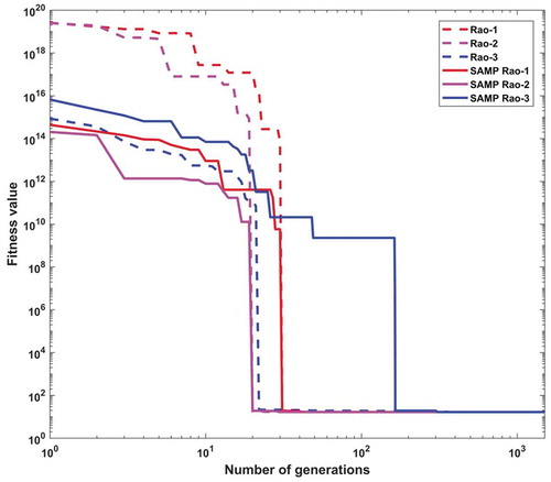
In the case of a spur gear train design problem, the optimal designs are obtained by considering two cases of search space as shown in the Appendix B. In both the cases, the population size and the maximum number of function evaluations are considered as 10 and 1,000, respectively, in each Rao and SAMP-Rao algorithm. Table 31 exhibits the optimal designs obtained for compact search space, i.e., case 1 of this problem. The optimal designs obtained by SAMP-Rao algorithms and Rao-2 are the same as shown in Table 16. Also, SAMP-Rao algorithms have required less function evaluations than corresponding Rao algorithms to get the optimum solution for this problem. The optimal designs obtained using SA, PSO, and GWO are infeasible due to violation of its design constraint(s). So the optimal designs obtained in case 1 of this problem using SAMP-Rao algorithms are superior to the optimal designs obtained using GA, SA, PSO, GWO, and Rao algorithms. Also, the computational time taken by SAMP-Rao algorithms is very less than SA and PSO algorithms, and there is very small difference between the time taken by Rao and SAMP-Rao algorithms for this problem. Figure 29 illustrates the speed of convergence of Rao and SAMP-Rao algorithms to reach the optimal solution for case 1 of this problem. For this problem, the convergence speed of the SAMP-Rao-1 algorithm is better and it has converged first to optimum solution at the 26th generation.

Table 31. Optimal designs of a spur gear train in compact search space (case 1).

Design variables	Algorithm
	GA*	SA*	PSO*	GWO*	Rao-1	Rao-2	Rao-3	SAMP Rao-1	SAMP Rao-2	SAMP Rao-3
fmin	3,512.6	3,127.71^a	3,127.7^a	3,094.8626^a	3,134.247907	3,134.247895	3,134.247896	3,134.247895	3,134.247895	3,134.247895
b	24	23.7	23.7	23.9031	23.90306526	23.90306511	23.90306511	23.903065	23.903065	23.90306511
d1	30	30	30	30	30	30	30	30	30	30
d2	30	36.761	36.763	30	36.73591229	36.73591223	36.73591229	36.735912	36.735912	36.7359
Z1	18	18	18	18	18	18	18	18	18	18
m	2.75	2.75	2.75	2.75	2.75	2.75	2.75	2.75	2.75	2.75
Active constraints	NA	1,4	1,4	1,3	1,4	1,4	1,4	1,4	1,4	1,4
maxFEs	20,000	2,200	1,000	9,000	1,000	1,000	1,000	1,000	1,000	1,000
FEs	NA	NA	NA	7,569	960	970	990	940	950	980
NP	20	NA	20	30	10	10	10	10	10	10
Time taken (s)	NA	5.23	1.79	NA	0.2	0.24	0.21	0.26	0.28	0.27

*GA (Yokota, Taguchi, and Gen 1998); SA and PSO (Savsani, Rao, and Vakharia 2010); GWO (Dorterler, Sahin, and Gokce 2019).

^aInfeasible solution due to violation of constraint(s).

Figure 29. Convergence plot for the spur gear train problem with compact search space.

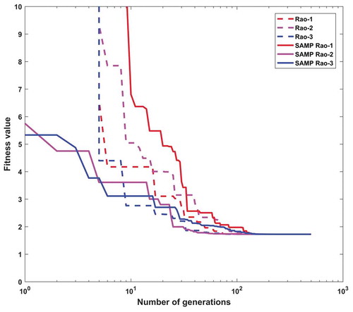
In case 2 of a spur gear train design problem, the optimal designs obtained using SAMP-Rao algorithms are the same as shown in Table 32. The optimal design obtained using GWO is infeasible due to the violation of its design constraint(s). So the optimal designs obtained in case 2 of this problem using SAMP-Rao algorithms are superior to the optimal designs obtained using SA, PSO, GWO and Rao algorithms. Also, the computational time taken by SAMP-Rao algorithms is less than SA and PSO algorithms, and there is very small difference between the time taken by Rao and SAMP-Rao algorithms for this problem. Figure 30 illustrates the speed of convergence of Rao and SAMP-Rao algorithms to reach the optimal solution for case 1 of this problem. For this problem, the convergence speed of the SAMP-Rao-1 algorithm is better and it has converged first to optimum solution at the 30th generation.

Table 32. Optimal designs of a spur gear train in expanded search space (case 2).

Design variables	Algorithm
	SA*	PSO*	GWO*	Rao-1	Rao-2	Rao-3	SAMP Rao-1	SAMP Rao-2	SAMP Rao-3
fmin	3,094.61	3,094.6	2,714.1645^a	2,993.166033	2,993.166040	2,993.166034	2,993.166030	2,993.166029	2,993.166030
b	32	32	35	33.89379939	33.89379939	33.89379937	33.893799	33.893799	33.893799
d1	30	30	29.97	30	30	30	30	30	30
d2	36.756	36.759	17.1614	36.7359	36.7359	36.7359	36.735912	36.735912	36.735912
Z1	25	25	23	24	24	24	24	24	24
m	2	2	2	2	2	2	2	2	2
Active constraints	1,4	1,4	3	1,4	1,4	1,4	1,4	1,4	1,4
maxFEs	2,200	1,000	9,000	1,000	1,000	1,000	1,000	1,000	1,000
FEs	NA	NA	5,200	1,000	1,000	950	980	1,000	950
NP	NA	20	30	10	10	10	10	10	10
Time taken (sec)	6.08	1.94	NA	0.2	0.24	0.22	0.28	0.32	0.3

* SA and PSO (Savsani, Rao, and Vakharia 2010); GWO (Dorterler, Sahin, and Gokce 2019).

^aInfeasible solution due to violation of a constraint.

Figure 30. Convergence plot for the spur gear train problem with expanded search space.

The proposed SAMP-Rao algorithms have provided better or competitive solutions for the constrained complex engineering design problems as compared to the other advanced optimization algorithms. Furthermore, the computational results of constrained engineering design problems have shown that the proposed SAMP-Rao algorithms have the ability to obtain better solutions for real-world constrained optimization problems in less number of iterations. The comparison of results has shown the effectiveness and robustness of SAMP-Rao algorithms over the other considered algorithms.

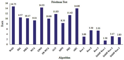
Furthermore, the performance of the proposed algorithms for the considered engineering design problems is validated using the Friedman rank test explained earlier. Table 33 presents the average rank of the algorithms provided by the Friedman test considering engineering design problems 1–6. From Table 33, it can be observed that the rank of SAMP-Rao algorithms is better than the corresponding Rao algorithms as well as the other algorithms considered. The SAMP-Rao-1 algorithm has obtained first rank among 16 algorithms with an average score of 1.5. As the p-value of the Friedman test is very less than 0.05, it confirms the high significance of proposed SAMP-Rao algorithms over the other algorithms for the design problems 1–6. Figure 31 presents the Friedman ranks of algorithms considered for the design problems 1–6 on a column chart. From Figure 31, it can be observed that the performance ranking of the algorithms for the design problems 1–6 is: SAMP-Rao-1, SAMP-Rao-3, Rao-1, SAMP-Rao-2, Rao-3, Rao-2, MFO, WCA, ER-WCA, MBA, SSA, PSO, ALO, ABC, GWO, and at last WAO.

Table 33. Friedman rank test for engineering design problems 1–6.

Algorithm	WAO	SSA	MBA	WCA	GWO	ER-WCA	ALO	MFO	PSO	ABC	Rao-1	Rao-2	Rao-3	SAMP Rao-1	SAMP Rao-2	SAMP Rao-3
Friedman ranks	14.75	10.50	10.17	9.33	14.33	10.00	11.83	8.33	11.42	14.00	3.00	5.50	5.33	1.50	3.17	2.83
χ^2	77.173
p-value	0.00001 (<0.05)

Figure 31. Friedman rank test for engineering design problems 1–6.

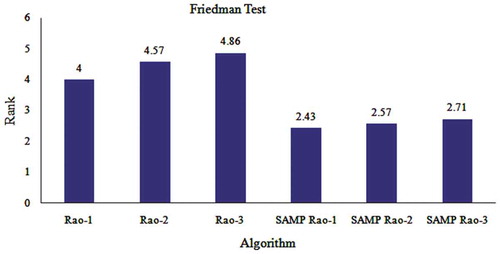
Table 34 presents the average rank of the considered algorithms provided by Friedman test considering engineering design problems 7–13. From Table 34, it can be observed that the rank of SAMP-Rao algorithms is better than the corresponding basic Rao algorithms. The SAMP-Rao-1 algorithm has obtained the first rank among the 6 algorithms with an average score of 2.43. As the p-value of the Friedman test is less than 0.05, it confirms the significance of proposed SAMP-Rao algorithms over Rao algorithms for the design problems 7–13. Figure 32 presents the Friedman ranks of algorithms considered for the design problems 7–32 on a column chart. From Figure 32, it can be observed that the performance ranking of the algorithms for the design problems 7–13 is: SAMP-Rao-1, SAMP-Rao-2, SAMP-Rao-3, Rao-1, Rao-2, and Rao-3.

Table 34. Friedman rank test for engineering design problems 7–13.

Algorithm	Rao-1	Rao-2	Rao-3	SAMP Rao-1	SAMP Rao-2	SAMP Rao-3
Friedman ranks	4	4.57	4.86	2.43	2.57	2.71
χ^2	13.735
p-value	0.0174 (<0.05)

Figure 32. Friedman rank test for engineering design problems 7–13.

Conclusions

In this work, the self-adaptive multi-population Rao algorithms are proposed. The performance of the proposed algorithms is explored over 25 unconstrained benchmark problems and 14 constrained engineering design optimization problems having a number of constraints and mixed type (continuous, discrete, and integer) design variables. From the comparison of results, it can be concluded that the proposed algorithms are effective and robust than the other optimization algorithms considered by the previous researchers for solving the benchmark problems as well as the complex constrained engineering design problems. The performance of the proposed algorithms is validated using the Friedman rank test and it can be concluded that the performance of proposed algorithms is significant than the other algorithms considered. The concept of SAMP-Rao algorithms is very simple and they are not having any algorithm-specific control parameters to be tuned. In the proposed algorithms, the basic Rao algorithms are upgraded using multi-population search process. The diversity of search is improved due to multi-population search scheme. Also, the exploration and exploitation rates of search process have been maintained with adaptive change of multi-population based on fitness values. In addition, the proposed algorithms have the potential to handle mixed-type design variables while satisfying a number of complex design constraints simultaneously. Furthermore, the computational complexity of basic Rao algorithms is reduced with the help of proposed SAMP-Rao algorithms. In future studies, the proposed algorithms will be used to solve other engineering design optimization problems. Also, multi-objective engineering design optimization problems will be attempted using the proposed algorithms.

Appendix A

Table 35. Unconstrained benchmark functions considered.

No.	Function	Formulation	D	Search range	C
F1	Sphere	$F_1(y)=\sum _{i=1}^D{y}_i^2$	30	[−100,100]	US
F2	SumSquares	$F_2(y)=\sum _{i=1}^{D}i{y}_i^2$	30	[−10,10]	US
F3	Beale	$F_3(y)=\sum _{i=1}^D{\left(1.5-y_1+y_1{y}_2\right)}^2+{\left(2.25-y_1+y_1{y}_2^2\right)}^2+{\left(2.625-y_1+y_1{y}_2^3\right)}^2$	2	[−4.5,4.5]	UN
F4	Easom	$F_4(y)=-cos(y_1)cos(y_2)exp(-(y_1-\pi {)}^2-(y_2-\pi {)}^2)$	2	[−100,100]	UN
F5	Matyas	$F_5(y)=0.26(y_1^2+y_2^2)-0.48y_1{y}_2$	2	[−10,10]	UN
F6	Colville	$\begin{array}{rl}& F_6(y)=100(y_1^2-y_2{)}^2+(y_1-1{)}^2+(y_3-1{)}^2-90(y_3^2-y_4)+\\ & 10.1\left({(y_2-1)}^2+{(y_4-1)}^2\right)+19.8(y_2-1)(y_4-1)\end{array}$	4	[−10,10]	UN
F7	Trid 6	$F_7(y)=\sum _{i=1}^D{(y_i-1)}^2-\sum _{i=2}^D{y}_i{y}_{i-1}$	6	[-D^2,D^2]	UN
F8	Trid 10	$F_8(y)=\sum _{i=1}^D{(y_i-1)}^2-\sum _{i=2}^D{y}_i{y}_{i-1}$	10	[-D^2,D^2]	UN
F9	Zakharov	$F_9(y)=\sum _{i=1}^D{y_i^2+\left(\sum _{i=1}^{D}0.5i{y}_i\right)}^2+{\left(\sum _{i=1}^{D}0.5i{y}_i\right)}^4$	10	[−5,10]	UN
F10	Schwefel 1.2	$F_{10}(y)=\sum _{i=1}^D{\left(\sum _{j=1}^i{y}_j^2\right)}^2$	30	[−100,100]	UN
F11	Rosenbrock	$F_{11}(y)=\sum _{i=1}^D\left[100{\left(y_i^2-y_{i+1}\right)}^2+{\left(1-y_i\right)}^2\right]$	30	[−30,30]	UN
F12	Dixon-Price	$F_{12}(y)={\left(y_i-1\right)}^2+\sum _{i=2}^{D}i{\left(2y_i^2-y_{i-1}\right)}^2$	30	[−10,10]	UN
F13	Branin	2	[−5,10] [0,15]	MS
F14	Bohachevsky 1	$F_{14}(y)=y_1^2+2y_2^2-0.3cos\left(3\pi y_1\right)-0.4cos\left(4\pi y_2\right)+0.7$	2	[−100,100]	MS
F15	Bohachevsky 2	$F_{15}(y)=y_1^2+2y_2^2-0.3cos\left(3\pi y_1\right)\left(4\pi y_2\right)+0.3$	2	[−100,100]	MN
F16	Bohachevsky 3	$F_{16}(y)=y_1^2+2y_2^2-0.3cos\left(3\pi y_1+4\pi y_2\right)+0.3$	2	[−100,100]	MN
F17	Booth	$F_{17}(y)={\left(y_1+2y_2-7\right)}^2+{\left(2y_1+y_2-5\right)}^2$	2	[−10,10]	MS
F18	Michalewicz 2	$F_{18}(y)=-\sum _{i=1}^{D}sin{y}_1{\left(sin\left(i{y}_i^2/\pi \right)\right)}^{20}$	2	[0,π]	MS
F19	Michalewicz 5	$F_{19}(y)=-\sum _{i=1}^{D}sin{y}_1{\left(sin\left(i{y}_i^2/\pi \right)\right)}^{20}$	5	[0,π]	MS
F20	GoldStein-Price	$\begin{array}{rl}& F_{20}(y)=\left[1+{\left(y_1+y_2+1\right)}^2\left(19-14y_1+3y_1^2-14y_2+6y_1{y}_2+3y_2^2\right)\right]\\ & \left[30+{\left(2y_1-3y_2\right)}^2\left(18-32y_1+12y_1^2+48y_2-36y_1{y}_2+27y_2^2\right)\right]\end{array}$	2	[−2,2]	MN
F21	Perm	$F_{21}(y)=\sum _{k=1}^D{\left[\sum _{i=1}^D\left(i^k+\beta \right)\left({\left(y_i/i\right)}^k-1\right)\right]}^2$	4	[-D,D]	MN
F22	Ackley	$F_{22}(y)=-20exp\left(-0.2\sqrt{\frac{1}{D}\sum _{i=1}^D{y}_i^2}\right)-exp\left(\frac{1}{D}\sum _{i=1}^{D}cos2\pi y_i\right)+20+e$	30	[−32,32]	MN
F23	Shekel’s Foxholes	$F_{23}(y)=\left[\frac{1}{500}+\sum _{j=1}^{25}\frac{1}{j+\sum _{i=1}^2{\left(y_i-a_{ij}\right)}^6}\right]$	2	[−65.536,65.536]	MS
F24	Hartmann 3	$F_{24}(y)=-\sum _{i=1}^4{c}_{i}exp\left[-\sum _{j=1}^3{a}_{ij}{\left(y_j-p_{ij}\right)}^2\right]$	3	[0,1]	MN
F25	Penalized 2	$\begin{array}{rl}& F_{25}(y)=0.1\left[{sin}^2\left(\pi y_1\right)+\sum _{i=1}^{D-1}\begin{array}{c}{\left(y_i-1\right)}^2\left\{1+{sin}^2\left(3\pi y_{i+1}\right)\right\}\\ +{\left(y_D-1\right)}^2+\left(1+{sin}^2\left(2\pi y_D\right)\right)\end{array}\right]\\ & \begin{array}{ccc}\hspace{0.17em}& \hspace{0.17em}& \end{array}+\sum _{i=1}^{D}u\left(y_i,5,100,4\right),\begin{array}{ccc}\hspace{0.17em}& \hspace{0.17em}& \hspace{0.17em}\end{array}u\left(y_i,a,k,m\right)=\left\{\begin{array}{c}k{\left(y_i-a\right)}^m\begin{array}{cc}\hspace{0.17em}& \hspace{0.17em}\end{array}{y}_i\succ a,\\ 0\begin{array}{ccc}\begin{array}{cc}\hspace{0.17em}& \hspace{0.17em}\end{array}& \hspace{0.17em}& \hspace{0.17em}\end{array}-a\le y_i\le a,\\ k{\left(-y_i-a\right)}^m\begin{array}{cc}\hspace{0.17em}& \hspace{0.17em}\end{array}{y}_i\prec -a\end{array}\right\}\end{array}$	30	[−50,50]	MN

D, dimension; C, characteristics; U, unimodal; M, multimodal; S, separable, N, nonseparable.

Appendix B.

Formulations of the considered engineering design optimization problems

Problem 1: Belleville spring

(B.1) $\mathrm{D}\mathrm{e}\mathrm{s}\mathrm{i}\mathrm{g}\mathrm{n}\mathrm{v}\mathrm{a}\mathrm{r}\mathrm{i}\mathrm{a}\mathrm{b}\mathrm{l}\mathrm{e}\mathrm{s},\left\{x\right\}=\left[D_o,D_i,t,h\right]$(B.1)

Objective function:

(B.2) $f(x)=0.07075\pi \left(D_o^2-D_i^2\right)t$(B.2)

Design constraints:

(B.3) $C_1\left(x\right)=\frac{4E{\delta }_{max}}{(1-{\mu }^2)\alpha D_e^2}\left[\beta \left(h-0.5{\delta }_{max}\right)+\gamma .t\right]\le \sigma$(B.3)

(B.4) $C_2\left(x\right)=\frac{4E{\delta }_{max}}{(1-{\mu }^2)\alpha D_e^2}\left[\left(h-0.5{\delta }_{max}\right)\left(h-{\delta }_{max}\right)t+t^3\right]\ge P_{max}$(B.4)

(B.5) $C_3\left(x\right)={\delta }_l\ge {\delta }_{max};C_4\left(x\right)=H-t\ge h;$(B.5)

(B.6) $C_5\left(x\right)=D_o\le D_{max};C_6\left(x\right)=D_o\ge D_i;$(B.6)

(B.7) $C_7\left(x\right)=\left(\frac{h}{D_o-D_i}\right)\le 0.3$(B.7)

(B.8) $5\le D_o\le 15;5\le D_i\le 15;0.2\le t\le 0.25;0.2\le h\le 0.25$(B.8)

(B.9) $\mathrm{w}\mathrm{h}\mathrm{e}\mathrm{r}\mathrm{e}K=\frac{D_o}{D_i};\alpha =\frac{6}{\pi ln(K)}{\left(\frac{K-1}{K}\right)}^2;$(B.9)

(B.10) $\beta =\frac{6}{\pi ln(K)}\left(\frac{K-1}{ln(K)}-1\right);\gamma =\frac{6}{\pi ln(K)}\left(\frac{K-1}{2}\right)$(B.10)

(B.11) $a=\frac{h}{t};{\delta }_l=h\times f(a);P_{max}=5400lb;{\delta }_{max}=0.2in;$(B.11)

(B.12) $\sigma =200kPsi;E=30e6Psi;\mu =0.3;H=2in;$(B.12)

(B.13) $D_{max}=12.01in.$(B.13)

Problem 2: Car side impact design

(B.14) $\mathrm{D}\mathrm{e}\mathrm{s}\mathrm{i}\mathrm{g}\mathrm{n}\mathrm{v}\mathrm{a}\mathrm{r}\mathrm{i}\mathrm{a}\mathrm{b}\mathrm{l}\mathrm{e}\mathrm{s},\left\{x\right\}=\left[x_1,x_2,x_3,x_4,x_5,x_6,x_7,x_8,x_9,x_{10},x_{11}\right]$(B.14)

Objective function:

(B.15) $f(x)=4.9x_1+6.67x_2+6.98x_3+4.01x_4+1.78x_5+2.73x_7+1.98$(B.15)

Design constraints:

(B.16) $\begin{array}{rl}& C_1(x)=0.3717x_2{x}_4+0.00931x_2{x}_{10}+0.484x_3{x}_9\\ & -0.01343x_6{x}_{10}+0.16\ge 0\end{array}$(B.16)

(B.17) $\begin{array}{rl}& C_2(x)=0.0159x_1{x}_2+0.188x_1{x}_8+0.019x_2{x}_7-0.0144x_3{x}_5\\ & -0.0008757x_5{x}_{10}-0.080405x_6{x}_9-0.00139x_8{x}_{11}\\ & -0.00001575x_{10}{x}_{11}+0.059\ge 0\end{array}$(B.17)

(B.18) $\begin{array}{rl}& C_3(x)=0.106-0.00817x_5+0.131x_1{x}_8+0.0704x_1{x}_9\\ & -0.03099x_2{x}_6+0.018x_2{x}_7-0.0208x_3{x}_8\\ & -0.121x_3{x}_9+0.00364x_5{x}_6-0.0007715x_5{x}_{10}\\ & +0.0005354x_6{x}_{10}-0.00121x_8{x}_{11}\ge 0\end{array}$(B.18)

(B.19) $\begin{array}{rl}& C_4(x)=0.246+0.061x_2+0.163x_3{x}_8-0.001232x_3{x}_{10}\\ & +0.166x_7{x}_9-0.227x_2^2\ge 0\end{array}$(B.19)

(B.20) $\begin{array}{rl}& C_5(x)=3.02+4.2x_1{x}_2-3.818x_3-0.0207x_5{x}_{10}\\ & +7.7x_7{x}_8-6.63x_6{x}_9-0.32x_9{x}_{10}\ge 0\end{array}$(B.20)

(B.21) $\begin{array}{rl}& C_6(x)=-1.86+5.057x_1{x}_2-2.95x_3+11x_2{x}_8-0.1792x_{10}\\ & +9.98x_7{x}_8+0.0215x_5{x}_{10}-22x_8{x}_9\ge 0\end{array}$(B.21)

(B.22) $C_7(x)=12.9x_1{x}_8+9.9x_2-0.1107x_3{x}_{10}-14.36\ge 0$(B.22)

(B.23) $\begin{array}{rl}& C_8(x)=-0.72+0.5x_4+0.19x_2{x}_3+0.0122x_4{x}_{10}\\ & -0.009325x_6{x}_{10}-0.000191x_{11}^2\ge 0\end{array}$(B.23)

(B.24) $\begin{array}{rl}& C_9(x)=-0.68+0.674x_1{x}_2-0.02054x_3{x}_{10}+1.95x_2{x}_8\\ & -0.028x_6{x}_{10}+0.0198x_4{x}_{10}\ge 0\end{array}$(B.24)

(B.25) $\begin{array}{rl}& C_{10}(x)=-0.75+0.489x_3{x}_7+0.843x_5{x}_6+0.0556x_9{x}_{11}\\ & -0.0432x_9{x}_{10}+0.000786x_{11}^2\ge 0\end{array}$(B.25)

(B.26) $\mathrm{w}\mathrm{h}\mathrm{e}\mathrm{r}\mathrm{e}0.5\le x_i\le 1.5\mathrm{f}\mathrm{o}\mathrm{r}i=1,\dots \dots .,7$(B.26)

(B.27) $x_8,x_9\in \left[0.192,0.345\right]\mathrm{a}\mathrm{n}\mathrm{d}-30\le x_{10},x_{11}\le 30$(B.27)

Problem 3: Coupling with a bolted rim

(B.28) $\mathrm{D}\mathrm{e}\mathrm{s}\mathrm{i}\mathrm{g}\mathrm{n}\mathrm{v}\mathrm{a}\mathrm{r}\mathrm{i}\mathrm{a}\mathrm{b}\mathrm{l}\mathrm{e}\mathrm{s},\left\{x\right\}=\left[d,N,R_B,M\right]$(B.28)

Objective function:

(B.29) $f(x)={\beta }_1\left(\frac{R_B+{\phi }_4(d)+c}{R_M}\right)+{\beta }_2\left(\frac{N}{N_M}\right)+{\beta }_3\left(\frac{M}{M_T}\right)$(B.29)

Design constraints:

(B.30) $C_1(x)=K(d)-\frac{\alpha M}{N{R}_B}\ge 0;C_2(x)=\frac{2\pi R_B}{N}-{\varphi }_5(d)\ge 0$(B.30)

(B.31) $C_3(x)=R_B-R_M-{\varphi }_4(d)\ge 0;C_4(x)=d-6\ge 0$(B.31)

(B.32) $C_5(x)=24-d\ge 0;C_6(x)=N-N_M\ge 0$(B.32)

(B.33) $C_7(x)=N_{max}-N\ge 0;C_8(x)=R_B-R_M\ge 0$(B.33)

(B.34) $C_9(x)=R_{max}-R_B\ge 0;C_{10}(x)=M-M_T\ge 0$(B.34)

(B.35) $C_{11}(x)=M_{max}-M\ge 0$(B.35)

(B.36) $\mathrm{w}\mathrm{h}\mathrm{e}\mathrm{r}\mathrm{e}{K}_d(x)=\frac{0.9f_m{R}_e\pi {\left[{\varphi }_1\left(d\right)\right]}^2}{4\sqrt{1+3{\left[\frac{4\left(0.16{\varphi }_3\left(d\right)+0.583{\varphi }_2\left(d\right)f_1\right)}{{\varphi }_1\left(d\right)}\right]}^2}}$(B.36)

(B.37) $\alpha =1.5;R_e=627MPa;M_T=40Nm;M_{max}=100Nm$(B.37)

(B.38) $c=5mm;N_M=8;N_{max}=100;{\beta }_1={\beta }_2={\beta }_3=1$(B.38)

(B.39) $R_M=50mm;R_{max}=100mm;6\le d\le 24$(B.39)

(B.40) $50\le R_B\le 100;8\le N\le 100;40\le M\le 100$(B.40)

Problem 4: Rolling element bearing

(B.41) $\mathrm{D}\mathrm{e}\mathrm{s}\mathrm{i}\mathrm{g}\mathrm{n}\mathrm{v}\mathrm{a}\mathrm{r}\mathrm{i}\mathrm{a}\mathrm{b}\mathrm{l}\mathrm{e}\mathrm{s},\left\{x\right\}=\left[D_m,D_b,f_i,f_o,Z,K_{Dmin},K_{Dmax},\beta ,\epsilon ,e\right]$(B.41)

Objective function:

(B.42) $f\left(x\right)=C_d=\left\{\begin{array}{c}{f}_c{Z}^{2/3}{D_b}^{1.8}if{D}_b\le 25.4mm\\ 3.647f_c{Z}^{2/3}{D_b}^{1.4}if{D}_b>25.4mm\end{array}\right.$(B.42)

where

(B.43) $fc=37.91{\left[1+{\left\{1.04{\left(\frac{1-\gamma }{1+\gamma }\right)}^{1.72}{\left(\frac{f_i\left(2f_o-1\right)}{f_o\left(2f_o-1\right)}\right)}^{0.41}\right\}}^{10/3}\right]}^{-0.3}\left[\frac{{\gamma }^{0.3}{\left(1-\gamma \right)}^{1.39}}{{\left(1+\gamma \right)}^{1/3}}\right]{\left[\frac{2f_i}{2f_i-1}\right]}^{0.41}$(B.43)

(B.44) $\gamma =D_{b}cos\alpha /D_m(Here\alpha =0)$(B.44)

Design constraints:

(B.45) $C_1\left(x\right)=\frac{{\phi }_0}{2{sin}^{-1}\left(D_b/D_m\right)}+1\ge Z$(B.45)

(B.46) $C_2\left(x\right)=2D_b-\left(D-d\right)K_{Dmin}\ge 0$(B.46)

(B.47) $C_3\left(x\right)=\left(D-d\right)K_{Dmax}-2D_b\ge 0$(B.47)

(B.48) $C_4\left(x\right)=\beta w-D_b\ge 0$(B.48)

(B.49) $C_5\left(x\right)=D_m-\left(D+d\right)\left(0.5-e\right)\ge 0$(B.49)

(B.50) $C_6\left(x\right)=\left(D+d\right)\left(0.5+e\right)-D_m\ge 0$(B.50)

(B.51) $C_7\left(x\right)=0.5\left(D-D_b-D_m\right)-\left(\epsilon \times D_b\right)\ge 0$(B.51)

(B.52) $C_8\left(x\right)=f_i-0.515\ge 0$(B.52)

(B.53) $C_9\left(x\right)=f_o-0.515\ge 0$(B.53)

where

(B.54) ${\phi }_0=2\pi -2{cos}^{-1}\left[\frac{{\left(\frac{D}{2}-T-D_b\right)}^2-{\left(\frac{d}{2}+T\right)}^2+U^2}{2\left(\frac{D}{2}-T-D_b\right)U}\right]$(B.54)

(B.55) $T=\frac{D-d-2D_b}{4};U=\frac{D-d}{2}-3T$(B.55)

(B.56) $D=160;d=90;w=30$(B.56)

(B.57) $0.5(D+d)\le D_m\le 0.6(D+d);0.15(D-d)\le D_b\le 0.45(D-d)$(B.57)

(B.58) $0.515\le f_i\le 0.6;0.515\le f_o\le 0.6;4\le Z\le 50$(B.58)

(B.59) $0.4\le K_{Dmin}^{\hspace{0.17em}}\le 0.5;0.6\le K_{Dmax}^{\hspace{0.17em}}\le 0.7;0.3\le \epsilon \le 0.4$(B.59)

(B.60) $0.02\le e\le 0.1;0.6\le \beta \le 0.85$(B.60)

Problem 5: Speed reducer

(B.61) $\mathrm{D}\mathrm{e}\mathrm{s}\mathrm{i}\mathrm{g}\mathrm{n}\mathrm{v}\mathrm{a}\mathrm{r}\mathrm{i}\mathrm{a}\mathrm{b}\mathrm{l}\mathrm{e}\mathrm{s},\left\{x\right\}=\left[b,m,Z,l_1,l_2,d_1,d_2\right]$(B.61)

Objective function:

(B.62) $\begin{array}{rl}& f\left(x\right)=0.7854b{m}^2\left(3.3333Z^2+14.9334Z-43.0934\right)\\ & \begin{array}{cc}\hspace{0.17em}& \hspace{0.17em}\end{array}\begin{array}{cc}\hspace{0.17em}& \hspace{0.17em}\end{array}-1.508b\left(d_1^2+d_2^2\right)+7.4777\left(d_1^3+d_2^3\right)\\ & \begin{array}{cc}\hspace{0.17em}& \hspace{0.17em}\end{array}\begin{array}{cc}\hspace{0.17em}& \hspace{0.17em}\end{array}+0.7854\left(l_1{d}_1^2+l_2{d}_2^2\right)\end{array}$(B.62)

Design constraints:

(B.63) $C_1\left(x\right)=27-b{m}^{2}Z\le 0$(B.63)

(B.64) $C_2\left(x\right)=397.5-b{m}^2{Z}^2\le 0$(B.64)

(B.65) $C_3\left(x\right)=1.93l_1^3-mZ{d}_1^4\le 0$(B.65)

(B.66) $C_4\left(x\right)=1.93l_2^3-mZ{d}_2^4\le 0$(B.66)

(B.67) $C_5\left(x\right)=\sqrt{{\left(745l_1/mZ\right)}^2+(16.9\times {10}^6)}-110d_1^3\le 0$(B.67)

(B.68) $C_6\left(x\right)=\sqrt{{\left(745l_2/mZ\right)}^2+(157.5\times {10}^6)}-85d_2^3\le 0$(B.68)

(B.69) $C_7\left(x\right)=mZ-40\le 0$(B.69)

(B.70) $C_8\left(x\right)=5m-b\le 0$(B.70)

(B.71) $C_9\left(x\right)=b-12m\le 0$(B.71)

(B.72) $C_{10}\left(x\right)=1.5d_1-l_1+1.9\le 0$(B.72)

(B.73) $C_{11}\left(x\right)=1.1d_2-l_2+1.9\le 0$(B.73)

(B.74) $2.6\le b\le 3.6,0.7\le m\le 0.8,17\le Z\le 28,7.3\le l_1\le 8.3,$(B.74)

(B.75) $7.8\le l_2\le 8.3,2.9\le d_1\le 3.9,5\le d_2\le 5.5$(B.75)

Problem 6: Step-cone pulley

(B.76) $\mathrm{D}\mathrm{e}\mathrm{s}\mathrm{i}\mathrm{g}\mathrm{n}\mathrm{v}\mathrm{a}\mathrm{r}\mathrm{i}\mathrm{a}\mathrm{b}\mathrm{l}\mathrm{e}\mathrm{s},\left\{x\right\}=\left[d_1,d_2,d_3,d_4,w\right]$(B.76)

Objective function:

(B.77) $f(x)=\frac{\pi }{4}\rho w\left\{\begin{array}{c}{d}_1^2\left[1+{\left(\frac{N_1}{N}\right)}^2\right]+d_2^2\left[1+{\left(\frac{N_2}{N}\right)}^2\right]+\\ d_3^2\left[1+{\left(\frac{N_3}{N}\right)}^2\right]+d_4^2\left[1+{\left(\frac{N_4}{N}\right)}^2\right]\end{array}\right\}$(B.77)

Design constraints:

(B.78) $C_1\left(x\right)=c_1-c_2=0$(B.78)

(B.79) $C_2\left(x\right)=c_1-c_3=0$(B.79)

(B.80) $C_3\left(x\right)=c_1-c_4=0$(B.80)

(B.81) $C_{4,5,6,7}\left(x\right)=R_i-2\ge 0\begin{array}{cc}\hspace{0.17em}& \hspace{0.17em}\end{array}i=1,...,4$(B.81)

(B.82) $C_{8,9,10,11}\left(x\right)=P_i-(0.75\times 745.6998)\ge 0\begin{array}{cc}\hspace{0.17em}& \hspace{0.17em}\end{array}i=1,...,4$(B.82)

where

c_i is the belt length to obtain speed N_i and can be calculated by

(B.83) $c_i=\frac{\pi d_i}{2}\left(\frac{N_i}{N}+1\right)+\frac{{\left(\frac{N_i}{N}-1\right)}^2{d}_i^2}{4a}+2a\begin{array}{cc}\hspace{0.17em}& \hspace{0.17em}\end{array}i=1,...,4$(B.83)

R_i is the tension ratio and can be calculated by

(B.84) $R_i=exp\left\{\mu \left[\pi -2{sin}^{-1}\left\{\frac{d_i}{2a}\left(\frac{N_i}{N}-1\right)\right\}\right]\right\}\begin{array}{cc}\hspace{0.17em}& \hspace{0.17em}\end{array}i=1,...,4$(B.84)

P_i is the power transmitted at each step and can be calculated by

(B.85) $\begin{array}{rl}& P_i=stw\left[1-exp\left\{-\mu \left[\pi -2{sin}^{-1}\left\{\frac{d_i}{2a}\left(\frac{N_i}{N}-1\right)\right\}\right]\right\}\right]\times \left(\frac{\pi d_i{N}_i}{60}\right)\\ & \begin{array}{cc}\hspace{0.17em}& \hspace{0.17em}\end{array}\begin{array}{cc}\hspace{0.17em}& \hspace{0.17em}\end{array}\begin{array}{cc}\hspace{0.17em}& \hspace{0.17em}\end{array}\begin{array}{cc}\hspace{0.17em}& \hspace{0.17em}\end{array}\begin{array}{cc}\hspace{0.17em}& \hspace{0.17em}\end{array}\begin{array}{cc}\hspace{0.17em}& \hspace{0.17em}\end{array}\begin{array}{cccc}\hspace{0.17em}& \hspace{0.17em}& \hspace{0.17em}& \hspace{0.17em}\end{array}\begin{array}{cccc}\hspace{0.17em}& \hspace{0.17em}& \hspace{0.17em}& \hspace{0.17em}\end{array}i=1,...,4\end{array}$(B.85)

(B.86) $\rho =7200kg/m^3;\mu =0.35;a=3m;t=8mm;s=1.75MPa$(B.86)

(B.87) $16\le w\le 100;40\le d_i\le 100\begin{array}{cc}\hspace{0.17em}& \hspace{0.17em}\end{array}i=1,...,4.$(B.87)

Problem 7: Welded beam

(B.88) $\mathrm{D}\mathrm{e}\mathrm{s}\mathrm{i}\mathrm{g}\mathrm{n}\mathrm{v}\mathrm{a}\mathrm{r}\mathrm{i}\mathrm{a}\mathrm{b}\mathrm{l}\mathrm{e}\mathrm{s},\vec{x}=\left[x_1,x_2,x_3,x_4\right]=\left[h,l,t,b\right]$(B.88)

Objective function:

(B.89) $\mathrm{M}\mathrm{i}\mathrm{n}\mathrm{i}\mathrm{m}\mathrm{i}\mathrm{z}\mathrm{e}f\left(\vec{x}\right)=1.10471x_1^2{x}_2+0.04811x_3{x}_4\left(14.0+x_2\right)$(B.89)

Design constraints:

(B.90) $C_1\left(\vec{x}\right)=\tau \left(\vec{x}\right)-{\tau }_{max}\le 0$(B.90)

(B.91) $C_2\left(\vec{x}\right)=\sigma \left(\vec{x}\right)-{\sigma }_{max}\le 0$(B.91)

(B.92) $C_3\left(\vec{x}\right)=P-P_c\left(\vec{x}\right)\le 0$(B.92)

(B.93) $C_4\left(\vec{x}\right)=\delta \left(\vec{x}\right)-{\delta }_{max}\le 0$(B.93)

(B.94) $C_5\left(\vec{x}\right)=x_1-x_4\le 0$(B.94)

(B.96) $C_6\left(\vec{x}\right)=0.125-x_1\le 0$(B.96)

(B.97) $C_7\left(\vec{x}\right)=0.10471x_1^2+0.04811x_3{x}_4(14.0+x_2)-5.0\le 0$(B.97)

(B.98) $0.1\le x_1\le 2,0.1\le x_2\le 10,0.1\le x_3\le 10,0.1\le x_4\le 2$(B.98)

where,

(B.100) $\tau \left(\vec{x}\right)=\sqrt{{({\tau }^{\prime })}^2+2{\tau }^{\prime }\tau \frac{x_2}{2R}+{(\tau )}^2}$(B.100)

(B.101) ${\tau }^{\prime }=\frac{P}{\sqrt{2}{x}_1{x}_2};\tau =\frac{MR}{J};M=P\left(L+\frac{x_2}{2}\right)$(B.101)

(B.102) $R=\sqrt{\frac{x_2^2}{4}+{\left(\frac{x_1+x_3}{2}\right)}^2}$(B.102)

(B.103) $J=2\left\{\sqrt{2}{x}_1{x}_2\left[\frac{x_2^2}{12}+{\left(\frac{x_1+x_3}{2}\right)}^2\right]\right\}$(B.103)

(B.104) $\sigma \left(\vec{x}\right)=\frac{6PL}{x_4{x}_3^2};\delta \left(\vec{x}\right)=\frac{4P{L}^3}{E{x}_3^3{x}_4}$(B.104)

$P_c\left(\vec{x}\right)=\frac{4.013E\sqrt{\frac{x_3^2{x}_4^6}{36}}}{L^2}\left(1-\frac{x_3}{2L}\sqrt{\frac{E}{4G}}\right)$

$\begin{array}{rl}& P=6000lb,L=14in,E=30\times {10}^{6}psi,G=12\times {10}^{6}psi,\\ & {\sigma }_{max}=30000psi,{\tau }_{max}=13600psi,{\delta }_{max}=0.25in\end{array}$

Problem 8: I-beam

(B.106) $\mathrm{D}\mathrm{e}\mathrm{s}\mathrm{i}\mathrm{g}\mathrm{n}\mathrm{v}\mathrm{a}\mathrm{r}\mathrm{i}\mathrm{a}\mathrm{b}\mathrm{l}\mathrm{e}\mathrm{s},\vec{x}=\left[x_1,x_2,x_3,x_4\right]=\left[b,h,t_w,t_h\right]$(B.106)

Objective function:

(B.107) $\mathrm{M}\mathrm{i}\mathrm{n}\mathrm{i}\mathrm{m}\mathrm{i}\mathrm{z}\mathrm{e}f\left(\vec{x}\right)=\frac{5000}{\frac{t_w{\left(h-2t_f\right)}^3}{12}+\frac{b{t}_f^3}{6}+2b{t}_f{\left(\frac{h-t_f}{2}\right)}^2}$(B.107)

Design constraint:

(B.108) $C_1\left(\vec{x}\right)=2b{t}_w+t_w(h-2t_f)\le 300$(B.108)

(B.109) $10\le x_1\le 50,10\le x_2\le 80,0.9\le x_3\le 5,0.9\le x_4\le 5$(B.109)

Problem 9: Cantilever beam

(B.110) $\mathrm{D}\mathrm{e}\mathrm{s}\mathrm{i}\mathrm{g}\mathrm{n}\mathrm{v}\mathrm{a}\mathrm{r}\mathrm{i}\mathrm{a}\mathrm{b}\mathrm{l}\mathrm{e}\mathrm{s},\vec{x}=\left[x_1,x_2,x_3,x_4,x_5\right]$(B.110)

Objective function:

(B.111) $\mathrm{M}\mathrm{i}\mathrm{n}\mathrm{i}\mathrm{m}\mathrm{i}\mathrm{z}\mathrm{e}f\left(\vec{x}\right)=0.0624(x_1+x_2+x_3+x_4+x_5)$(B.111)

Design constraint:

(B.112) $C_1\left(\vec{x}\right)=\frac{61}{x_1^3}+\frac{37}{x_2^3}+\frac{19}{x_3^3}+\frac{7}{x_4^3}+\frac{1}{x_5^3}\le 1$(B.112)

(B.113) $0.01\le x_i\le 100\mathrm{f}\mathrm{o}\mathrm{r}\mathrm{i}=1,2,3,4,5$(B.113)

Problem 10: Tension/compression spring

(B.114) $\mathrm{D}\mathrm{e}\mathrm{s}\mathrm{i}\mathrm{g}\mathrm{n}\mathrm{v}\mathrm{a}\mathrm{r}\mathrm{i}\mathrm{a}\mathrm{b}\mathrm{l}\mathrm{e}\mathrm{s},\vec{x}=\left[x_1,x_2,x_3\right]=\left[d,D,N\right]$(B.114)

Objective function:

(B.115) $\mathrm{M}\mathrm{i}\mathrm{n}\mathrm{i}\mathrm{m}\mathrm{i}\mathrm{z}\mathrm{e}f\left(\vec{x}\right)=(x_3+2)x_2{x}_1^2$(B.115)

Design constraints:

(B.116) $C_1\left(\vec{x}\right)=71785x_1^4-x_2^3{x}_3\le 0$(B.116)

(B.117) $C_2\left(\vec{x}\right)=\frac{4x_2^2-x_1{x}_2}{12566(x_2{x}_1^3-x_1^4)}+\frac{1}{5108x_1^2}-1\le 0$(B.117)

(B.118) $C_3\left(\vec{x}\right)=x_2^2{x}_3-140.45x_1\le 0$(B.118)

(B.119) $C_4\left(\vec{x}\right)=x_1+x_2-1.5\le 0$(B.119)

(B.120) $0.05\le x_1\le 2,0.25\le x_2\le 1.3,2\le x_3\le 15$(B.120)

Problem 11: Pressure vessel

(B.121) $\mathrm{D}\mathrm{e}\mathrm{s}\mathrm{i}\mathrm{g}\mathrm{n}\mathrm{v}\mathrm{a}\mathrm{r}\mathrm{i}\mathrm{a}\mathrm{b}\mathrm{l}\mathrm{e}\mathrm{s},\vec{x}=\left[x_1,x_2,x_3,x_4\right]=\left[T_s,T_h,R,L\right]$(B.121)

Objective function:

(B.122) $\mathrm{M}\mathrm{i}\mathrm{n}\mathrm{i}\mathrm{m}\mathrm{i}\mathrm{z}\mathrm{e}f\left(\vec{x}\right)=0.6224x_1{x}_3{x}_4+1.7781x_2{x}_3^2+3.1661x_1^2{x}_4+19.84x_1^2{x}_3$(B.122)

Design constraints:

(B.123) $C_1\left(\vec{x}\right)=0.0193x_3-x_1\le 0$(B.123)

(B.124) $C_2\left(\vec{x}\right)=0.00954x_3-x_2\le 0$(B.124)

(B.125) $C_3\left(\vec{x}\right)=1296000-\pi x_3^2{x}_4-\frac{4}{3}\pi x_3^3\le 0$(B.125)

(B.126) $C_4\left(\vec{x}\right)=x_4-240\le 0$(B.126)

(B.127) $x_1,x_2\in \left[0.0625,0.125,.......,1.1875,1.25\right],10\le x_3,x_4\le 200$(B.127)

Problem 12: Gear train

(B.128) $\mathrm{D}\mathrm{e}\mathrm{s}\mathrm{i}\mathrm{g}\mathrm{n}\mathrm{v}\mathrm{a}\mathrm{r}\mathrm{i}\mathrm{a}\mathrm{b}\mathrm{l}\mathrm{e}\mathrm{s},\vec{x}=\left[x_1,x_2,x_3,x_4\right]=\left[n_A,n_B,n_C,n_D\right]$(B.128)

Objective function:

(B.129) $\mathrm{M}\mathrm{i}\mathrm{n}\mathrm{i}\mathrm{m}\mathrm{i}\mathrm{z}\mathrm{e}f\left(\vec{x}\right)={\left(\frac{1}{6.931}-\frac{x_3{x}_2}{x_1{x}_4}\right)}^2$(B.129)

(B.130) $\mathrm{s}\mathrm{u}\mathrm{b}\mathrm{j}\mathrm{e}\mathrm{c}\mathrm{t}\mathrm{t}\mathrm{o}:12\le x_1,x_2,x_3,x_4\le 60$(B.130)

Problem 13: 3-bar truss

Design variables,

(B.131) $\vec{x}=\left[x_1,x_2\right]=\left[A_1,A_2\right]$(B.131)

Objective function:

(B.132) $\mathrm{M}\mathrm{i}\mathrm{n}\mathrm{i}\mathrm{m}\mathrm{i}\mathrm{z}\mathrm{e}f\left(\vec{x}\right)=\left(2\sqrt{2}{x}_1+x_2\right)\times L$(B.132)

Design constraints:

(B.133) $C_1\left(\vec{x}\right)=\left(\sqrt{2}{x}_1+x_2\right)P-\sigma \left(\sqrt{2}{x}_1^2+2x_1{x}_2\right)\le 0$(B.133)

(B.134) $C_2\left(\vec{x}\right)=x_{2}P-\sigma \left(\sqrt{2}{x}_1^2+2x_1{x}_2\right)\le 0$(B.134)

(B.135) $C_3\left(\vec{x}\right)=P-\sigma \left(\sqrt{2}{x}_2+x_1\right)\le 0$(B.135)

(B.136) $0\le x_1,x_2\le 1$(B.136)

where $L=100cm,$ $P=2KN/c{m}^2$ and $\sigma =2KN/c{m}^2$

Problem 14: Spur gear train

(B.137) $\mathrm{D}\mathrm{e}\mathrm{s}\mathrm{i}\mathrm{g}\mathrm{n}\mathrm{v}\mathrm{a}\mathrm{r}\mathrm{i}\mathrm{a}\mathrm{b}\mathrm{l}\mathrm{e}\mathrm{s},\left\{x\right\}=\left[b,Z_1,d_1,d_2,m\right]$(B.137)

Objective function:

(B.138) $f\left(x\right)=\frac{\pi }{4}\frac{\rho }{1000}\left[b{Z}_1^2{m}^2\left(a^2+1\right)-\left(D_i^2-d_o^2\right)\left(l-b_w\right)-n{b}_w{d}_p^2-b\left(d_1^2+d_2^2\right)\right]$(B.138)

Design constraints:

(B.139) $C_1(x)=b_1\le F_s$(B.139)

(B.140) $C_2(x)=b_2\le \left(F_s/F_p\right)$(B.140)

(B.141) $C_3(x)=b_3\le d_1^3$(B.141)

(B.142) $C_4(x)=b_4\le d_2^3$(B.142)

(B.143) $C_5(x)=b_5-\frac{Z_1(1+a)m}{2}\ge 0$(B.143)

(B.144) $\mathrm{w}\mathrm{h}\mathrm{e}\mathrm{r}\mathrm{e}a=4,\rho =8mg/m^3,P=7.5kW,n=6$(B.144)

(B.145) $N_1=1500rpm,b_w=3.5m,l_w=2.5m,D_r=am{Z}_1-2.5m$(B.145)

(B.146) $d_o=d_2+25,D_i=D_r-2l_w,D_1=m{Z}_1,D_2=am{Z}_1$(B.146)

(B.147) $d_p=0.25(D_i-d_o),N_2=N_1/a,Z_2=Z_1{D}_2/D_1$(B.147)

(B.148) $v=\pi D_1{N}_1/60000,b_5=151.5,b_4=(48.68e6P)/N_2\tau$(B.148)

(B.149) $b_3=(48.68e6P)/N_1\tau ,b_1=(1000P/v),K_v=0.389$(B.149)

(B.150) $K_w=0.8,\sigma =294.3MPa,\tau =19.62MPa,y=0.102$(B.150)

(B.151) $F_s=\pi K_v{K}_{w}bmy\sigma ,F_p=2K_v{K}_{w}b{D}_1{Z}_2/(Z_1+Z_2)$(B.151)

Ranges of design variables:

(B.152) $\mathrm{C}\mathrm{a}\mathrm{s}\mathrm{e}1:20\le b\le 32,10\le d_1\le 30,30\le d_2\le 40$(B.152)

(B.153) $18\le Z_1\le 25\mathrm{a}\mathrm{n}\mathrm{d}m=\left[2.75,3,3.5,4\right]$(B.153)

(B.154) $\mathrm{C}\mathrm{a}\mathrm{s}\mathrm{e}2:10\le b\le 35,10\le d_1\le 30,10\le d_2\le 40$(B.154)

(B.155) $18\le Z_1\le 25\mathrm{a}\mathrm{n}\mathrm{d}m=\left[1,1.25,1.5,2,2.75,3,3.5,4\right]$(B.155)

References

- Awad, N. H., M. Z. Ali, P. N. Suganthan, J. J. Liang, and B. Y. Qu. 2016. Problem definitions and evaluation criteria for the CEC 2017 special session and competition on single objective real-parameter numerical optimization. Technical report, Nanyang Technological University, Singapore.
- Chowdhury, S., M. Marufuzzaman, H. Tunc, L. Bian, and W. Bullington. 2019. A modified ant colony optimization algorithm to solve a dynamic travelling salesman problem: A case study with drones for wildlife surveillance. Journal of Computational Design and Engineering 6:368–86. doi:10.1016/j.jcde.2018.10.004.
- Coello, C. A. C. 2000. Treating constraints as objectives for single-objective evolutionary optimization. Engineering Optimization 32 (3):275–308. doi:10.1080/03052150008941301.
- Derrac, J., S. Garcia, D. Molina, and F. Herrera. 2011. A practical tutorial on the use of nonparametric statistical tests as a methodology for comparing evolutionary and swarm intelligence algorithms. Swarm and Evolutionary Computation 1:3–18. doi:10.1016/j.swevo.2011.02.002.
- Dorterler, M., I. Sahin, and H. Gokce. 2019. A grey wolf optimizer approach for optimal weight design problem of the spur gear. Engineering Optimization 51 (6):1013–27. doi:10.1080/0305215X.2018.1509963.
- Gandomi, A. H., X. Yang, and A. H. Alavi. 2013. Cuckoo search algorithm: A metaheuristic approach to solve structural optimization problems. Engineering with Computers 29:17–35. doi:10.1007/s00366-011-0241-y.
- Gu, L., R. J. Yang, C. H. Tho, M. Makowskit, O. Faruquet, and Y. Lit. 2001. Optimization and robustness for crashworthiness of side impact. International Journal of Vehicle Design 26 (4):348–60. doi:10.1504/IJVD.2001.005210.
- Gulcu, S., and H. Kodaz. 2015. A novel parallel multi-swarm algorithm based on comprehensive learning particle swarm optimization. Engineering Applications of Artificial Intelligence 45:33–45. doi:10.1016/j.engappai.2015.06.013.
- Hashim, F. A., E. H. Houssein, M. S. Mabrouk, A. Walid, and S. Mirjalili. 2019. Henry gas solubility optimization: A novel physics-based algorithm. Future Generation Computer Systems 101:646–67. doi:10.1016/j.future.2019.07.015.
- Jena, P. K., D. N. Thatoi, and D. R. Parhi. 2015. Dynamically self-adaptive fuzzy PSO technique for smart diagnosis of transverse crack. Applied Artificial Intelligence 29 (3):211–32. doi:10.1080/08839514.2015.1004611.
- Li, C., T. T. Nguyen, M. Yang, S. Yang, and S. Zeng. 2015. Multi-population methods in un-constrained continuous dynamic environments: The challenges. Information Sciences 296:95–118. doi:10.1016/j.ins.2014.10.062.
- Li, C., and S. Yang. 2008. Fast multi-swarm optimization for dynamic optimization problems. In Proceedings of the Fourth International Conference on Natural Computation, ICNC’08, 7, Jinan, China, IEEE, 624–28. doi:10.1109/ICNC.2008.313
- Mirjalili, S. 2015a. Moth-flame optimization algorithm: A novel nature-inspired heuristic paradigm. Knowledge-based Systems 89:228–49. doi:10.1016/j.knosys.2015.07.006.
- Mirjalili, S. 2015b. The ant lion optimizer. Advances in Engineering Software 83:80–98. doi:10.1016/j.advengsoft.2015.01.010.
- Mirjalili, S., and A. Lewis. 2016. The whale optimization algorithm. Advances in Engineering Software 95:51–67. doi:10.1016/j.advengsoft.2016.01.008.
- Mirjalili, S., and S. M. Mirjalili. 2016. Multi-verse optimizer: A nature-inspired algorithm for global optimization. Neural Computing and Applications 27 (2):495–513. doi:10.1007/s00521-015-1870-7.
- Mirjalili, S., S. M. Mirjalili, and A. Lewis. 2014. Grey wolf optimizer. Advances in Engineering Software 69:46–61. doi:10.1016/j.advengsoft.2013.12.007.
- Mortazavi, A. 2019. Interactive fuzzy search algorithm: A new self-adaptive hybrid optimization algorithm. Engineering Applications of Artificial Intelligence 81:270–82. doi:10.1016/j.engappai.2019.03.005.
- Nseef, S. K., S. Abdullah, A. Turky, and G. Kendall. 2016. An adaptive multi-population artificial bee colony algorithm for dynamic optimisation problems. Knowledge-based Systems 104:14–23. doi:10.1016/j.knosys.2016.04.005.
- Rao, R. V. 2016. Jaya: A simple and new optimization algorithm for solving constrained and unconstrained optimization problems. International Journal of Industrial Engineering Computations 7 (1):19–34.
- Rao, R. V. 2019. Jaya: An advanced optimization algorithm and its engineering applications. Switzerland: Springer International Publishing.
- Rao, R. V. 2020. Rao algorithms: Three metaphor-less simple algorithms for solving optimization problems. International Journal of Industrial Engineering Computations 11:107–30. doi:10.5267/j.ijiec.2019.6.002.
- Rao, R. V., and V. K. Patel. 2013. Multi-objective optimization of heat exchangers using modified teaching-learning–Based optimization. Applied Mathematical Modelling 37 (3):1147–62. doi:10.1016/j.apm.2012.03.043.
- Rao, R. V., and A. Saroj. 2017. A self-adaptive multi-population based Jaya algorithm for engineering optimization. Swarm and Evolutionary Computation 37:1–26. doi:10.1016/j.swevo.2017.04.008.
- Rao, R. V., V. J. Savsani, and D. P. Vakharia. 2011. Teaching-learning-based optimization: A novel method for constrained mechanical design optimization problems. Computer-Aided Design 43 (3):303–15. doi:10.1016/j.cad.2010.12.015.
- Rizk-Allah, R. M. 2018. Hybridizing sine cosine algorithm with multi-orthogonal search strategy for engineering design problems. Journal of Computational Design and Engineering 5:249–73. doi:10.1016/j.jcde.2017.08.002.
- Savsani, V., R. V. Rao, and D. P. Vakharia. 2010. Optimal weight design of a gear train using particle swarm optimization and simulated annealing algorithms. Mechanism and Machine Theory 45:531–41. doi:10.1016/j.mechmachtheory.2009.10.010.
- Turky, A. M., and S. Abdullah. 2014. A multi-population harmony search algorithm with external archive for dynamic optimization problems. Information Sciences 272 (1):84–95. doi:10.1016/j.ins.2014.02.084.
- Vafashoar, R., and M. R. Meybodi. 2018. Multi swarm optimization algorithm with adaptive connectivity degree. Applied Intelligence 48:909–41. doi:10.1007/s10489-017-1039-4.
- Wang, S., Y. Li, and H. Yang. 2017. Self-adaptive differential evolution algorithm with improved mutation mode. Applied Intelligence 47:644–58. doi:10.1007/s10489-017-0914-3.
- Xia, L., J. Chu, and Z. Geng. 2014. A multiswarm competitive particle swarm algorithm for optimization control of an ethylene cracking furnace. Applied Artificial Intelligence 28 (1):30–46. doi:10.1080/08839514.2014.862772.
- Yang, S., and C. Li. 2010. A clustering particle swarm optimizer for locating and tracking multiple optima in dynamic environments. IEEE Transactions on Evolutionary Computation 14 (6):959–74. doi:10.1109/TEVC.2010.2046667.
- Yildiz, A. R., H. Abderazek, and S. Mirjalili. 2019. A comparative study of recent non-traditional methods for mechanical design optimization. Archives of Computational Methods in Engineering 1–18. doi:10.1007/s11831-019-09343-x
- Yokota, T., T. Taguchi, and M. Gen. 1998. A solution method for optimal weight design problem of the gear using genetic algorithms. Computers and Industrial Engineering 35 (3–4):523–26. doi:10.1016/S0360-8352(98)00149-1.
- Zarchi, D. A., and B. Vahidi. 2018. Multi objective self adaptive optimization method to maximize ampacity and minimize cost of underground cables. Journal of Computational Design and Engineering 5:401–08. doi:10.1016/j.jcde.2018.02.004.
- Zhang, J., and X. Ding. 2011. A multi-swarm self-adaptive and cooperative particle swarm optimization. Engineering Applications of Artificial Intelligence 24:958–67. doi:10.1016/j.engappai.2011.05.010.
- Zhao, Z., B. Liu, C. Zhang, and H. Liu. 2019. An improved adaptive NSGA-II with multi-population algorithm. Applied Intelligence 49:569–80. doi:10.1007/s10489-018-1263-6.