Comparison of Supervised Classifiers and Image Features for Crop Rows Segmentation on Aerial Images

ABSTRACT

In this paper we present a comparison of supervised classifiers and image features for crop row segmentation of aerial images captured from an unmanned aerial vehicle (UAV). The main goal is to investigate which methods are the most suitable to solve this specific problem, as well as to test quantitatively how well they perform for robust segmentation of row patterns. For this purpose, we conducted a systematic literature review over the recent methods specifically designed for aerial image crop row segmentation, and for comparison purposes we implemented the most prominent approaches. Most used Color-texture features were faced against most used classifiers, resulting into a total of 48 combinations, usually having their construction concepts based on the following two step-procedures: (i) supervised training step to build some model over the selected color-texture feature space which is also based upon user-selected samples from the input image; and (ii) classification step, where each pixel of the input image is classified employing the corresponding classifier. The obtained results were compared against a Ground-Truth (GT) image, performed by a human expert, using two distinct evaluation metrics, indicating the most suitable combination of color-texture descriptors and classifiers able to solve the segmentation problem of specific cultures obtained from UAV images.

Introduction

Precision agriculture is a relatively new application field characterized by the use of technology to increase productivity and quality of cultures while making use of policies to preserve the environment McBratney et al. (2005). There are several examples of precision agriculture tools, varying according to their application such as decision support systems for farm management, data management, pesticide/nutrient use optimization, crop marketing, telematics services, unmanned aerial vehicles (UAV), and others Reyns et al. (2002). Specifically, regarding UAVs, their use provides aerial images that allow inspecting a wide monitoring area, offering high-resolution imaging with varied multispectral channels (visible light and near, medium and far infrared channels).

Aerial images can be used in the most varied fields in precision agriculture. The identification of rows corresponding to the vegetation patterns in images may facilitate the optimization of chemicals spreading. Further tasks such as counting plants, rows length measurement, skips detection and weed management also provide relevant information that can be used to estimate the relative productivity of specific plantation zones, estimating their vigor, coverage, and density Torres-Sánchez, López-Granados, and Pen˜a (2015); Torres-Sánchez et al. (2014). Additionally, autonomous navigation ground vehicles such as tractors can be assisted by the row information gathered through UAVs, combined with other geographical and topographical data.

In order to be able to support precision agriculture through aerial imaging, precise and reliable quantitative analysis of agricultural images is necessary. This is usually done through computerized methods based on Computer Vision (CV) methods, employed as a toolbox of routines used for gathering data for the decision making procedure.

The vegetation rows identification, for example, consists in a pixel-wise classification problem (semantic segmentation), where each pixel is classified into crop row or background (soil/inter-row) area, providing a segmented image. Usually, when vegetation is confronted against soil, the high color variances makes easier to differentiate those classes. However, when in the presence of distinct evolutionary stages of a specific culture, or advanced stages with very dense vegetation covering, providing an accurate classification becomes a challenging problem.

Objectives

The objective of our work is to investigate the problem of vegetation row segmentation on aerial images and address it employing supervised classification methods. For this purpose, we:

• investigate which classifiers and features extractors are commonly used in the literature;

• implement the most common or promising;

• apply them to an UAV-acquired sugar cane orthomosaic dataset, using various combinations of information in their feature space;

• validate their performance against a ground truth produced by a biologist.

This paper is organized as follows: Section 2 provides an overview of the state of the art. In Section 3 the data set, classifiers, features extractors and validation methods used in our experiments are described. Results are presented in Section 4. Finally, discussion, conclusions and further works are presented in Section 5.

State of the Art

In order to obtain a state of the art related to vegetation row segmentation approaches, we performed a systematic literature review. The review was performed accordingly to the method for systematic literature review proposed in Kitchenham (2004).

The research main question asked in our approach is: Which methods of image segmentation, specifically designed for crop rows in aerial images, have already been proposed in scientific articles available over the literature? The research was conducted in 2018, for articles written in English Language, published between 2008 and 2018, which proposed some algorithm capable of segmenting plants into aerial images. The databases used in the research were Science Direct, IEEE and Springer. The search strings used, as well as the number of articles returned, are shown in the Table 1.

Table 1. Search string used on this systematic review.

Database	Search String	Retrieved Papers
Science Direct	(“unmanned aerial vehicle”) AND (“agriculture”) AND ((“crop” AND “row”) OR (“weed”) AND (“detection” OR “maping”))	103
IEEEXplore	((“unmanned aerial vehicle” AND “agriculture” AND “crop” AND “row”) OR “unmanned aerial vehicle” AND “agriculture” AND “weed” AND “mapping”)	121
Springer	(“weed detection”) OR (“weed detection” AND “unmaned aerial vehicles”)	139

To the 363 papers returned by our search strings, we applied the following exclusion and inclusion criteria:

• exclusion criteria: simple application case studies or review articles that did not propose any method or method modification tailored for the problem in question;

• inclusion criteria: articles that proposed an algorithm or method, which, at some stage, includes the segmentation of vegetation in aerial images of plantations;

Only 22 papers met these criteria. They are listed and classified accordingly to approach and method in Appendix A. Below we provide a summary of what we identified in these works.

The precision agriculture application of the reviewed works varies between the detection of vegetation row, skips in rows, crop rows center line, and weeds. For all of these applications, at some point, its solution method needs to segment the image into crop and some other classes.

Additionally, it is possible to divide the reviewed works in two main categories: (i) use object-based image analysis (OBIA) Torres-Sánchez, López-Granados, and Pen˜a (2015); Pérez-Ortiz et al. (2016b); de Souza et al. (2017); Gao et al. (2018), and (ii) the ones based on other approaches not OBIA-based. The concept behind OBIA consist in utilize a general segmentation algorithm to divide the image into several small partitions (objects), and then classify each object instead of each pixel Hossain and Chen (2019).

The principal computer vision difference between each work is the feature space used to describe the elements on the image (pixels or objects). A large amount of the founded works uses some kind of vegetation index as features. These features consist of intensity values calculated from the spectral information, representing the greenness of each pixel. The most common indexes are the Excess Green Index (ExG) for visible spectrum cameras, and Normalized Difference Vegetation Index (NDVI) for multispectral cameras Torres-Sánchez, López-Granados, and Peña (2015); Pérez-Ortiz et al. (2015), Pérez-Ortiz et al. (2016b)); de Souza et al. (2017); Comba et al. (2015); Gao et al. (2018); Sa et al. (2018); David, Charlemagne, and Ballado (2016); Pérez-Ortiz et al. (2016a); Lottes et al. (2017); Bah, Hafiane, and Canals (2017). Works that focus on OBIA uses several features to describe data. Vegetation indices represent color information, gray level co-occurrence matrices (GLCM) are commonly used to capture texture, and object area/shape is used to describe geometric information of detected objects.

In some works, the plantations covered contains quite spaced crop rows, making possible to segment them with a simple Otsu threshold Torres-Sánchez et al. (2014). These works usually use this threshold as a starting seed point, to execute a more robust method. It is possible to use this strategy to apply Hough transform Duda and Hart (1972); Rong-Chin and Tsai (1995) to detect the center line of plantation rows, and use this information as spacial features to detect inter-row weeds Pérez-Ortiz et al. (2015), Pérez-Ortiz et al. (2016b)); Gao et al. (2018).

For the classification step, the majority of revised methods employ a well-known supervised algorithm. Support vector machines, random forests and K-nearest neighbors were used in some works Castillejo-González et al. (2014); Pérez-Ortiz et al. (2015), Pérez-Ortiz et al. (2016b)); Dos Santos Ferreira et al. (2017); Ishida et al. (2018); Gao et al. (2018).

More recent works are making use of newer machine learning techniques (deep learning), like Convolutional Neural Network (CNN) Sa et al. (2018), Dos Santos Ferreira et al. (2017). These networks have shown a great advance in pattern recognition tasks. In addition to its good performance, they have the capability to automatically learn what features best describe the observed data Zeiler and Fergus (2014).

Material and Methods

To investigate the problem of vegetation row segmentation in aerial images we implemented the most used supervised classifications algorithms, and the most used image features extractors. To compare the performance of those classifiers with each possible feature described, we perform the following experiment. A UAV image of a sugar cane field was segmented several times using each classifier. Each classifier was tested with different combinations of features in their feature vector.

Orthomosaic Image

The data set used in our experiments was build as follows. We employed a single UAV-acquired sugar cane field orthomosaic as our dataset. The image was captured from a Horus Aeronaves¹ fixed-wing UAV with a camera model canon G9X with a resolution of 20.4 megapixels. The UAV captured the data following a flight altitude of 125 to 200 meters, resulting in a resolution of $5cm/pixel$.

Ground Truth

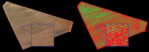
From the data set, an expert biologist produced a human-made ground truth (GT). The expert classified all pixels of the image manually, using the GNU image manipulation program (GIMP),² into two classes: crop row and background. Figure 1 presents the orthomosaic and the corresponding GT.³

Figure 1.: The left image shows the sugar cane Orthomosaic. The right image present the ground truth, whereas green = crop row area, and red = background area.

Classifiers

Our literature review showed that support vector machine (SVM), random forest (RF), Mahalanobis classifier (MC) and K-nearest neighbors (KNN) are commonly used supervised algorithms, for this kind of pixel classification problem.

K-Nearest Neighbors

Possibly the simplest supervised classification machine learning algorithm, the KNN classifier is a type of instance-based learning, or lazy learning, where the training data is simply recorded and no model is created based on train data Cover and Hart (1967). The classification of unclassified data is done by voting between the K nearest samples in the train data. The most common distance function used to calculate the nearest samples is the Euclidean distance. Hyperparameter K has to be chosen upon the data. Larger values of K can be used to reduces the effect of noise on train data but can make boundaries between classes less distinct.

The KNN classifier was used in this comparative study as a base method. It was chosen because it is a classic and quite simple method. Two K values were used, a small one and a larger one (three and eleven respectively).

Mahalanobis Distance

Mahalanobis distance is a distance metric based on the correlation between the vector components of a data sample. Given two arbitrary vector coordinates $u$ and $g$, and a data sample of vector coordinates $C$ with same dimensionality as $u$ and $g$, the Mahalanobis distance (MD) is computed by:

(1) $MD(u,g)={\left({\left(u-g\right)}^T{A}^{-1}\left(u-g\right)\right)}^{1/2}=\parallel u-g{\parallel }_A$(1)

where $A^{-1}$ is the inverse of the co-variance matrix obtained from $C$. The MD is a dual metric: if $A$ is an identity matrix, MD is reduced to the $L_2$-norm. As a main characteristic, the statistical distance presents an elliptic topology which surrounds the center of $C$.

An interesting variation of the MD is the Polynomial Mahalanobis Distance (PMD). The PMD was proposed by Grudic and Mulligan (2006) as a distance metric that has the ability to capture the non-linear characteristics of a multivariate distribution as a global metric. The degree of the polynomial ($q$-order) determines how rigorous the distance will be, based on the samples of the input distribution. A first-order PMD has the same effect as a simple MD.

The Mahalanobis distance, in both its linear and higher-order polynomial variations, has been shown to produce better results than linear color-metric approaches such as RGB or CIELab, when employed as a customized color-metric in various segmentation algorithms Lopes et al. (2016); Carvalho et al. (2015), Carvalho et al. (2014)); Sobieranski et al. (2014a); Sobieranski, Comunello, and von Wangenheim. (2011); Sobieranski et al. (2009a); Sobieranski et al. (2009b).

The methodology using the Mahalanobis Classifier consists, in the training step, to generate a different distance metrics (PMD) for each class present in the training set. The classification step consists of finding the closest class mean, using their respective distance metrics. We used the first three polynomial orders on our experiments.

Support Vector Machines

Probably one of the most popular classifier algorithms, support vector machines incrementally approximate a data classifier trying to create hyperplanes that best separate the data set into their classes. The best hyperplane must maximize the margin between the extreme points in each class. These extreme points that define the hyperplane are called support vectors Jakkula (2006). Since this method tries to separate the data employing hyperplanes, the classification can only work on linearly separable data. To overcome this limitation, a nonlinear kernel function is applied in the data set, transforming the feature space in a nonlinear high-dimensional projection, where it is linearly separable. The most popular kernels are the polynomial and the radial basis function (RBF). In our experiments, we tested two kernels, a simple linear and the RBF kernel. The RBF kernel is described in equation 2.

(2) $K({\mathbf{X}}_{\mathbf{i}},{\mathbf{Y}}_{\mathbf{j}})=EXP(-\gamma ||{\mathbf{X}}_{\mathbf{i}}-{\mathbf{Y}}_{\mathbf{j}}|{|}^2)$(2)

Random Forests

Random forest uses ensemble learning (bootstrap aggregating or bagging) on multiples decision trees Breiman (2001). Each one of these trees contains internal nodes (condition nodes) and leaf nodes (decision nodes). Each condition node contains a simple rule using one feature from the feature vector, and each decision node contains a class label. The classification of an unlabeled data is done walking down the tree following each condition node until a leaf node is reached, outputting a class label.

The bagging method is used in a slightly different way, de-correlating the trees splitting the feature vector into random subsets of features. Each tree in the forest considers only a small subset of features rather than all of the features of the model (each subset has $\sqrt{n}$ features, where $n$ is the total number of features). This way, highly correlated trees are avoided.

Feature Space

For the features, we found that vegetation indices are almost unanimously used as color information, and gray level co-occurrence matrices (GLCM) are frequently used for texture features extractor. Since texture is important information to discriminate different objects with the same color (connected parallel crop rows for example), we decided to include another well know texture feature extractor in our experiments, Gabor filters.

Vegetation Indices

Since most crops present a green coloration, it is intuitive that color information can be a useful feature for the segmentation. A vegetation index (VI) consists of mathematical manipulation of the image spectral channels (RGB), to measure the greenness of a pixel. Various VI’s were proposed on the literature Wang, Zhang, and Wei (2019), the most present ones in our review were the excess green index (ExG), for RGB cameras, and the normalized difference vegetation index (NDVI), for cameras with near-infrared spectrum. In this work, we only used VI for RGB cameras. The ExG index is expressed by the Equation 3, where G, R, and B are the intensity values of each channel normalized by the sum of the three.

(3) $ExG=2G-R-B$(3)

Gabor Filters

Gabor filters are traditional texture descriptors proposed by Denis Gabor Gabor (1946). The texture is extracted from the image by a set of base functions, which can be employed to build a Gabor filter bank. Each base function is modulated by a specific scale and orientation, and a process of convolution of the filters with an image produces responses where the structure adapts with the scale and orientation analyzed. Gabor filters have been shown to help in performing texture-based image segmentation through integrated color-texture descriptors Ilea and Whelan (2011). Gabor filter-based segmentation approaches have also been shown to be easy to parallelize, implement in GPUs and use to perform fast color-texture-based image segmentation Sobieranski et al. (2014b). The Gabor filter can be expressed by the Equation 4, where $u_0$ and $\varphi$ respectively correspond to frequency, and the phase offset (in degrees). The standard deviation $\sigma$ determines the size of the Gaussian filed.

(4) $h(x,y)=exp\left\{-\frac{1}{2}\left[\frac{x^2}{{\sigma }_x^2}+\frac{y^2}{{\sigma }_y^2}\right]\right\}cos(2\pi u_{0}x+\varphi ).$(4)

Different orientations can be obtained employing a rigid rotation of the $x$-$y$ coordinate system with an angle value predefined by $\theta$, as follows:

(5) $x=x_{0}cos(\theta )+y_{0}sin(\theta ),y=y_{0}cos(\theta )-x_{0}sin(\theta )$(5)

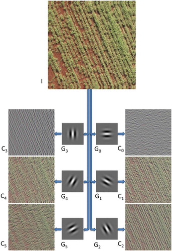
Figure 2 shows an example of processing an image $I$ by a Gabor Filter Bank $G_0...G_5$ composed of kernels presenting all the same amplitude and six different orientations.

Figure 2.: Image decomposition with a filter bank composed of six Gabor Kernels.

The Gabor filter bank used in our experiments was composed of 4 filters. The guidelines proposed in Jain and Farrokhnia (1991) were used to chose the Gabor features. We utilized frequencies values that generate kernels with a size that matches a crop row width. Only two orientations were used (0° and 90°) to reduce the feature vector size generated from the filter back.

Gray Level Co-Occurrence Matrix

Gray Level Co-Occurrence Matrix are second order statistic matrix used to extract texture information from an image Haralick, Shanmugam, and Dinstein (1973). This information is extracted from the image computing several co-occurrence matrices. A Gray Level Co-Occurrence Matrix $\mathbf{P}n\times n$, where $n$ is the number of gray levels of the image, is defined using the neighborhood of pixels, where ${\mathbf{P}}_{ij}$ is the probability of two neighbors pixels have intensities of $i$ and $j$. The neighborhood relationship is defined by an offset from the reference pixel. Different offsets can be used, a vertical GLCM can use $(1,0)$ and $(-1,0)$ offsets, and a horizontal one can use $(0,1)$ and $(0,-1)$. From each GLCM P, different texture features can be extracted, some of them are energy, entropy, contrast, dissimilarity, homogeneity, mean, standard deviation, and correlation.

For the experiments, we downsampled the input image from 8 bits per channel to 4 bits, so our GLCM’s have $16\times 16$ size. We used the most referenced features on our review, so we used five features: contrast, energy, mean, standard deviation, and correlation. Vertical and horizontal GLCM’s are used as offsets, with a window size of 33 pixels.

Validation Procedure

The combinations of features tested were done in an incremental form. First, feature vectors with only color information (RGB channels and vegetation indices), then color plus texture information (Gabor Filters and GLCM).

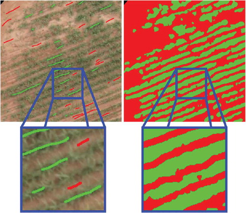
The training and classification step ware performed as follows. We manually selected some pixels as samples for each class and computed the feature vector (color and texture features) of each pixel. All the classifiers were then trained with the same train data. Once all classifiers were trained, the classification step was applied over the whole input images. Figure 3 shows one of the samples selected for training in this experiment and the ground truth of the corresponding portion of the image. For these images were considered as background the soil and inter-row areas.

Figure 3. Details of training sugar cane crop images: left image shows some samples selected for training, whereas green = crop row area, and red = soil/inter-row area. Right image illustrate the corresponding ground truth.

The validation of our results was performed through an automated quantitative comparison of our results against the GTs. The precision measures employed in our experiments were:

• the Jaccard index Everingham et al. (2010), also known as intersection-over-union index (IOU);

• the F1-score Van Rijsbergen (1979).

Results

The quantitative results obtained from the precision measures are demonstrated on Table 2. A total of 48 results were obtained, one from each combination of classifiers (with different parameters) and feature vectors. For each classifier, the feature vector that presented the best result has his result marked in bold. In the same way, for each feature vector, the best classifier has his result underlined.

Table 2. Precision measures for each combination of classifier and feature vector. The underlined values, in each column, represent the best result for the respective feature vector. The bold values, in each row, represent the best result for the respective classifier.

		RGB	RGB+EXG	RGB+GABOR	RGB+EXG+GABOR	RGB+GLCM	RGB+EXG+GLCM
Order 1	IOU	0.698119	0.697408	0.703623	0.692624	0.634717	0.630541
	F1	0.817026	0.816443	0.820750	0.812572	0.766440	0.762906
Order 2	IOU	0.701198	0.702799	0.712002	0.698958	0.527848	0.536951
	F1	0.819304	0.820475	0.827032	0.817356	0.666899	0.676264
Order 3	IOU	0.695696	0.699051	0.691902	0.691966	0.487234	0.494376
	F1	0.815242	0.817730	0.812188	0.812193	0.622772	0.630830
LSVM	IOU	0.749118	0.751493	0.771953	0.788654	0.460858	0.552117
	F1	0.853670	0.855305	0.869302	0.880129	0.624880	0.701774
SVMRBF	IOU	0.749793	0.744385	0.775278	0.781153	0.618053	0.581793
	F1	0.854297	0.850555	0.871527	0.875335	0.756181	0.724577
KNN3	IOU	0.736040	0.738847	0.760250	0.764573	0.561399	0.567494
	F1	0.844844	0.846798	0.861466	0.864365	0.710523	0.715644
KNN11	IOU	0.734586	0.738951	0.757570	0.762214	0.559606	0.565582
	F1	0.843771	0.846822	0.859617	0.862745	0.708793	0.713821
RF	IOU	0.700687	0.732188	0.663252	0.743981	0.646504	0.724697
	F1	0.819503	0.841898	0.791804	0.850180	0.779854	0.836857

The best observed result was archived using linear SVM with $RGB+EXG+GABOR$, reaching an F1 score precision of 0.88. This feature vector was the most interesting one, presenting the best results with almost every classifier. Both linear and RBF SVM had great results with little differences, for feature vector of color and Gabor features combinations. The RF classifier was the only one that was capable of make good use of GLCM features, showing the best results for this kind of feature vector.

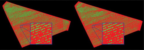
Figure 4 shows the result achieved on the entire field, with the linear SVM classifier and feature vector composed of $RGB+EXG+GABOR$. A visibly denser area can be noticed on the top part of the image, and a sparse one on the bottom part.

Figure 4. The left image shows the ground truth. The right image present the prediction archived with linear svm using RGB channels, EXG index and gabor features in the feature vector.

Discussion

This work performs a comparison of supervised classification technique, applied to the problem of crop row segmentation on aerial images. A systematic literature review was performed to find what methods are being used for this task. Four of the most common classifiers were selected and used on experiments. All classifiers were tested using several combinations of the most used features found on our review.

Our experiments were designed to measure, in a qualitative and quantitative manner, the precision of each method. Ground truth was generated by a biologist, that manually classified each pixel in sugar cane orthomosaic images. We employed the Jaccard index and the F1-score for the quantitative validation of the methods we tested because these are the most widely employed quantitative GT comparison measures in the area of semantic segmentation approaches that were published in the last years. This will allow researchers using this database, in the future, to also compare these approaches to CNN-based semantic segmentation approaches.

Classification Approaches and Decision Boundaries

One unexpected result was the poor performance of the segmentation employing the Mahalanobis distance as a classifier. Previous works had shown that the Mahalanobis distance, especially the non-linear higher order polynomial Mahalanobis distance, outperforms many other approaches when applied as a color-metric in different segmentation algorithms in the segmentation of both natural outdoors scenes and a varied set of medical imaging domains Lopes et al. (2016); Carvalho et al. (2015), Carvalho et al. (2014)); Sobieranski et al. (2014a); Sobieranski, Comunello, and von Wangenheim. (2011); Sobieranski et al. (2009a); Sobieranski et al. (2009b). In the application scenario we explored in this work this was clearly not the fall: both the linear and the polynomial Mahalanobis distances showed poorer results as other methods in most situations, with a best F1 of 82.7% and a best IoU of 71.2%, whereas LSVM obtained a F1 of 88.0% and an IoU of 78.8%. This, however, can be explained in the manner the Mahalanobis distance treats data: it is a statistic distance metric and relies on the mean value of the distribution of its samples. This means that, if the distribution is extremely convoluted, the mean can land outside the distribution and the Mahalanobis distance will lead to a description of the decision (hyper-)surfaces that can be even poorer as as a simple piece-wise linear kNN classifier.

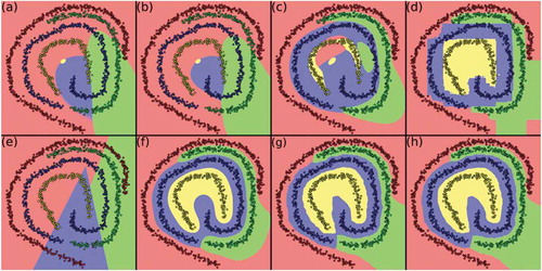
In order to illustrate the behavior of each classifier, we developed a simple software tool that produces a picture of the decision boundaries for any bi-dimensional hand generated data set and for any of the classifiers used in this work. Figure 5 shows a distribution of four 2-dimensional variables, with their samples depicted as data points. The colored surfaces are the decision surfaces and their boundaries, as generated by each of the classifiers we employed in this work. This tool was made freely available online, together with segmentation tools that can be used in order to reproduce the results described in this paper.⁴ The figure shows that linear and second-order polynomial Mahalanobis, together with linear SVM (a,b and e) cannot adequately represent the decision surfaces for these specific convoluted data distributions.

This shows that the decision, which classifier to use, depends strongly on the characteristics of the data. Since this sometimes is difficult to predict beforehand, to test an application with different combinations of classifiers and descriptors for the data seems to be indicated, as Table 2 indicates.

Figure 5. Decision Boundaries of hand generated data. (a):MC1, (b): MC2, (c): MC3, (d): RF, (e): SVM-Linear, (f): SVM-RBF, (g): KNN3, (h): KNN11.

Conclusions

The quantitative results showed that the combination of RGB, EXG and Gabor features generates the bests results, for the images used in our experiments, and the SVM methods outperformed the other ones when using this feature vector. A pixel-wise F1-score of 88.0% and an IoU of 78.8% indicate that classic color-texture-based image segmentation methods can still be considered an option for this application field, even with the present tendencies toward deep learning-based approaches. One of the advantages of this approach is that only a very simple and fast training is necessary, which can easily be achieved with a few manually generated examples, as shown in Figure 3. A deep learning semantic segmentation approach would demand the arduous creation of GTs similar to the ones we created for the validation of this work for each new kind of crop.

Further works should include an extensive validation with a richer and vast data set, containing other cultures besides sugar cane. Another state of the art computer vision approaches, like newer deep learning approaches, should be also included in future comparisons.

We made our dataset publicly available and the code used in our experiments is also available for download.⁵

Acknowledgments

This study was financed in part by the Coordenação de Aperfeiçoamento de Pessoal de Nível Superior - Brasil (CAPES) and by Fundação de Amparo à Pesquisa e Inovação do Estado de Santa Catarina (FAPESC). We also thank to Horus Aeronaves for support and data.

Notes

1. https://horusaeronaves.com/.

2. https://www.gimp.org/.

3. Dataset available for download at http://www.lapix.ufsc.br/crop-rows-sugar-cane.

4. https://codigos.ufsc.br/lapix/Tools-for-Supervised-Color-Texture-Segmentation-and-Results-Analysis.

5. https://codigos.ufsc.br/lapix/Tools-for-Supervised-Color-Texture-Segmentation-and-Results-Analysis.

Apependix A.

Systematic Literature Review Results

Table

Ref.	Author	Title	Detection Objective	Crop Type	Segmentation Method	Features
Torres- Sánchez, López- Granados, and Peña (2015)	Torres-Sánchez, López-Granados, and Peña 2015	An automatic object-based method for optimal thresholding in uav images: Application for vegetation detection in herbaceous crops	Vegetation detection	Herbaceous crops	Own threshold method based on Otsu.	EXG and NDVI indices
Torres-Sánchez et al. (2014)	Torres-Sánchez et al. 2014	Multi-temporal mapping of the vegetation fraction in early-season wheat fields using images from UAV	Vegetation detection	Wheat crops	Pixel based fixed threshold.	NGRDI, ExG, CIVE, VEG, ExGR, COM, COM2, and WI indices
Castillejo-González et al. (2014)	Castillejo-González, J.M. Pena- Barragán, M. Jurado-Expósito, F.J. Mesas-Carrascosa, F. López-Granados	Evaluation of pixel-and object-based approaches for mapping wild oat (Avena sterilis) weed patches in wheat fields using QuickBird imagery for site-specific management	Weed mapping	Wild oat in wheat crops	Supervised pixel and object classification. Comparison of several classifiers.	Spectral information (RGB-NIR)
Pérez-Ortiz et al. (2015)	Pérez-Ortiz et al. 2015	A semi-supervised system for weed mapping in sunflower crops using unmanned aerial vehicles and a crop row detection method	weed mapping	Sunflower crops	Pixel wise classification. Comparison of unsupervised, supervised and sime-supervised classifiers.	Spectral information (RGB-NIR), vegetation indices (EXG and NDVI) and hough lines transform crop row information
Pérez-Ortiz et al. (2016b)	Pérez-Ortiz et al. 2016b	Selecting patterns and features for between-and within-crop row weed mapping using uav-imagery	Weed mapping	Maize and sunflower crops	Object wise classification with SVM.	Vegetation Indices, histograms, GLCM, shape, proximity of plantation rows
de Souza et al. (2017)	de Souza et al. 2017	Mapping skips in sugar cane fields using object-based analysis of unmanned aerial vehicle (uav) images	Skip row mapping	sugar cane crops	Own OBIA procedure, developed on commercial software eCognition Developer 8.	NDVI index
Comba et al. (2015)	Comba et al. 2015	Vineyard detection from unmanned aerial systems images	Row detection	Vineyard crops	Dynamic local neighboring window segmentation procedure.	NDVI index
Gao et al. (2018)	Gao et al. 2018	Fusion of pixel and object-based features for weed mapping using unmanned aerial vehicle imagery	Weed Mapping	Maize crops	Object wise classification with Randon Forest.	Spectral RGB, vegetation index EXG, GLCM, geometrical and textural features and hough lines transform crop row information
Dos Santos Ferreira et al. (2017)	A. dos Santos Ferreira, D.M. Freitas, G.G. da Silva,H. Pistori, M.T. Folhes	Weed detection in soybean crops using ConvNets	Weed mapping	Soybean crops	Object wise classification with a convolutional neural network.	(GLCM), local binary patterns, histogram of oriented gradients (HOG) and RGB, HSV and CIELab color spaces
Ishida et al. (2018)	T. Ishida, J. Kurihara, F.A. Viray, S.B. Namuco, E.C. Pa-ringit, G.J. Perez, Y. Takahashi, J.J. Marciano Jr	A novel approach for vegetation classification using UAV-based hyperspectral imaging	Vegetation classification	Mango orchard	Pixel wise classification with SVM.	Spectral information (33 spectral bands, ranging from 460 to 780 nm at 1 nm intervals)
Sa et al. (2018)	Sa et al. 2018	Weednet: Dense semantic weed classification using multispectral images and mav for smart farming	Weed mapping	Sugar beet crops	Pixel wise classification with a semantic segmentation convnet.	Spectral information (RGB) and vegetation index (NDVI)
David, Charlemagne, and Ballado (2016)	David, Charlemagne, and Ballado 2016	Vegetation indices and textures in object-based weed detection from uav imagery	Weed mapping	Eggplant, corn, string beans crops	Object wise classification with SVM.	Vegetation indices: ExG, VEG, ExGR, Woebbecke, COM, VAR, green. And GLCM
Pérez- Ortiz et al. (2016a)	Pérez-Ortiz et al. 2016a	Machine learning paradigms for weed mapping via unmanned aerial vehicles	Weed mapping	Sunflower crops	Machine learning methods for pixel wise classification.	Spectral information (RGB-NIR), vegetation indices (EXG and NDVI)
Lottes et al. (2017)	Lottes et al. 2017	Uav-based crop and weed classification for smart farming	Weed mapping	Sugar beet crops	Object wise classification with Random Forest.	EXG,NDVI, geometric features, hough lines transform crop row information, gradient representation, color space and texture
Bah, Hafiane, and Canals (2017)	Bah, Hafiane, and Canals 2017	Weeds detection in uav imagery using slic and the hough transform	Weed mapping	Unspecified	Segmentation with Simple Linear Iterative Clustering (SLIC). Object classification with own method.	ExG, hough lines transform crop row information
de Castro et al. (2012)	de Castro et al. 2012	Airborne multi-spectral imagery for mapping cruciferous weeds in cereal and legume crops	Weed mapping	Cruciferous weeds in bean, pea and wheat crops	Pixel wise classification with some supervised classifiers.	Vegetation indices (R/B, B/G, NDVI and RVI)
de Castro, López-Granados, and Jurado-Expósito. (2013)	de Castro, López-Granados, and Jurado-Expósito. 2013	Broad-scale cruciferous weed patch classification in winter wheat using QuickBird imagery for in-season site-specific control	Weed mapping	Cruciferous weed in wheat, peas, beans and olive orchards crops	Object wise classification with Maximum Likelihood Classifier	Four band ratios (B/G, R/G, NIR/B and NIR/G), NDVI, R/B and DVI
López- Granados et al. (2016b)	López-Granados, Torres-Sánchez, Serrano-Pérez, de Castro, Mesas-Carrascosa, Pena 2016	Early season weed mapping in sunflower using UAV technology: variability of herbicide treatment maps against weed thresholds	Weed mapping	Sunflower crops	Object wise classification with adapted Otsu and crop row detection.	Visible and NIR spectrum, ExG and NDVI
López- Granados et al. (2016a)	López-Granados, Torres-Sánchez, De Castro, Serrano-Pérez, Mesas-Carrascosa, Peña 2016	Object-based early monitoring of a grass weed in a grass crop using high resolution UAV imagery	Weed mapping	Grass crops	Object wise classification with adapted Otsu and crop row detection.	Spectral information and vegetation index (ExG and NDVI)
Louargant et al. (2017)	Louargant, Villette, Jones, Vigneau, Paoli, Gée 2017	Weed detection by UAV: Simulation of the impact of spectral mixing in multispectral images	Weed mapping	lamb’s quarters and thistle weeds in maize crops	Pixel wise unsupervised classification with K-means and mahalanobis distance.	NDVI index
Barrero and Perdomo (2018)	Barrero, Perdomo 2018	RGB and multispectral UAV image fusion for Gramineae weed detection in rice fields	Weed mapping	Rice crops	Pixel wise classification with multi layer perceptron neural network.	Spectral information (RGB) and Haar wavelet transform, GLCM
Rasmussen et al. (2018)	Rasmussen et al. 2018	Pre-harvest weed mapping of Cirsium arvense in wheat and barley with off-the-shelf UAVs	Weed mapping	Wheat and barley crops	Own threshold method for object wise classification.	Vegetation index (EXG)

References

- Bah, M. D., A. Hafiane, and R. Canals. 2017. Weeds detection in UAV imagery using SLIC and the hough transform. Image Processing Theory, Tools and Applications (IPTA), 2017 Seventh International Conference on, 1–6, Montreal, Canada: IEEE.
- Barrero, O., and S. A. Perdomo. 2018. RGB and multispectral UAV image fusion for Gramineae weed detection in rice fields. Precision Agriculture 19 (5):809–22. doi:10.1007/s11119-017-9558-x.
- Breiman, L. 2001. Random forests. Machine Learning 45 (1):5–32. doi:10.1023/A:1010933404324.
- Carvalho, L. E., S. L. Mantelli Neto, A. C. Sobieranski, E. Comunello, and A. von Wangenheim. 2015. Improving graph-based image segmentation using nonlinear color similarity metrics. International Journal of Image and Graphics 15 (04):1550018. doi:10.1142/S0219467815500187.
- Carvalho, L. E., S. L. Mantelli Neto, A. von Wangenheim, A. C. Sobieranski, L. Coser, and E. Comunello. 2014. Hybrid color segmentation method using a customized nonlinear similarity function. International Journal of Image and Graphics 14 (01n02):1450005. doi:10.1142/S0219467814500053.
- Castillejo-González, I. L., J. M. Pena-Barragán, M. Jurado-Expósito, F. J. Mesas-Carrascosa, and F. López-Granados. 2014. Evaluation of pixel-and object-based approaches for mapping wild oat (Avena sterilis) weed patches in wheat fields using QuickBird imagery for site-specific management. European Journal of Agronomy 59:57–66. doi:10.1016/j.eja.2014.05.009.
- Comba, L., P. Gay, J. Primicerio, and D. R. Aimonino. 2015. Vineyard detection from unmanned aerial systems images. Computers and Electronics in Agriculture 114:78–87. doi:10.1016/j.compag.2015.03.011.
- Cover, T., and P. Hart. 1967. Nearest neighbor pattern classification. IEEE Transactions on Information Theory 13 (1):21–27. doi:10.1109/TIT.1967.1053964.
- David, L., G. Charlemagne, and A. H. Ballado. 2016. Vegetation indices and textures in object-based weed detection from UAV imagery. Control System, Computing and Engineering (ICCSCE), 2016 6th IEEE International Conference on, 273–78, Penang, Malaysia: IEEE.
- de Castro, A. I., M. Jurado-Expósito, J. M. Peña-Barragán, and F. López-Granados. 2012. Airborne multi-spectral imagery for mapping cruciferous weeds in cereal and legume crops. Precision Agriculture 13 (3):302–21. doi:10.1007/s11119-011-9247-0.
- de Castro, A. I., F. López-Granados, and M. Jurado-Expósito. 2013. Broad-scale cruciferous weed patch classification in winter wheat using QuickBird imagery for in-season site-specific control. Precision Agriculture 14 (4):392–413. doi:10.1007/s11119-013-9304-y.
- de Souza, C. H. W., R. A. C. Lamparelli, J. V. Rocha, and P. S. G. Magalhães. 2017. Mapping skips in sugarcane fields using object-based analysis of unmanned aerial vehicle (UAV) images. Computers and Electronics in Agriculture 143:49–56. doi:10.1016/j.compag.2017.10.006.
- Dos Santos Ferreira, A., D. M. Freitas, G. G. da Silva, H. Pistori, and M. T. Folhes. 2017. Weed detection in soybean crops using ConvNets. Computers and Electronics in Agriculture 143:314–24. doi:10.1016/j.compag.2017.10.027.
- Duda, R. O., and P. E. Hart. 1972. Use of the hough transformation to detect lines and curves in pictures. Communications of the ACM 15 (1):11–15. doi:10.1145/361237.361242.
- Everingham, M., L. Van Gool, C. K. I. Williams, J. Winn, and A. Zisserman. 2010. The pascal visual object classes (voc) challenge. International Journal of Computer Vision 88 (2):303–38. doi:10.1007/s11263-009-0275-4.
- Gabor, D. 1946. Theory of communication. Part 1: The analysis of information. Journal of the Institution of Electrical Engineers-Part III: Radio and Communication Engineering 93 (26):429–41.
- Gao, J., W. Liao, D. Nuyttens, P. Lootens, J. Vangeyte, A. Pižurica, Y. He, and J. G. Pieters. 2018. Fusion of pixel and object-based features for weed mapping using unmanned aerial vehicle imagery. International Journal of Applied Earth Observation and Geoinformation 67:43–53. doi:10.1016/j.jag.2017.12.012.
- Grudic, G. Z., and J. Mulligan. 2006. Outdoor path labeling using polynomial mahalanobis distance. In Robotics: Science and systems. University of Pennsylvania, Philadelphia, Pennsylvania, USA.
- Haralick, R., K. Shanmugam, and I. Dinstein. 1973. Textural features for image classification. IEEE Transactions on Systems, Man, and Cybernetics SMC-3:610–21. doi:10.1109/TSMC.1973.4309314.
- Hossain, M. D., and D. Chen. 2019. Segmentation for Object-based image analysis (OBIA): A review of algorithms and challenges from remote sensing perspective. ISPRS Journal of Photogrammetry and Remote Sensing 150:115–34. doi:10.1016/j.isprsjprs.2019.02.009.
- Ilea, D. E., and P. F. Whelan. 2011. Image segmentation based on the integration of colour–texture descriptors—A review. Pattern Recognition 44 (10–11):2479–501. doi:10.1016/j.patcog.2011.03.005.
- Ishida, T., J. Kurihara, F. A. Viray, S. B. Namuco, E. C. Paringit, G. J. Perez, Y. Takahashi, and J. J. Marciano Jr. 2018. A novel approach for vegetation classification using UAV-based hyperspectral imaging. Computers and Electronics in Agriculture 144:80–85. doi:10.1016/j.compag.2017.11.027.
- Jain, A. K., and F. Farrokhnia. 1991. Unsupervised texture segmentation using Gabor filters. PR 24 (12):1167–86.
- Jakkula, V. 2006. Tutorial on support vector machine (svm). 37, School of EECS, Washington State University .
- Kitchenham, B. 2004. Procedures for performing systematic reviews. Keele University, Joint Technical Report TR/SE-0401 33 (2004):1–26.
- Lopes, M. D., A. C. Sobieranski, A. V. Wangenheim, and E. Comunello. 2016. A web-based tool for semi-automated segmentation of histopathological images using nonlinear color classifiers. 2016 IEEE 29th International Symposium on Computer-Based Medical Systems (CBMS), Dublin and Belfast, Ireland, June, 247–52.
- López-Granados, F., J. Torres-Sánchez, A. I. D. C. Angélica Serrano-Pérez, F.-J. Mesas-Carrascosa, and J.-M. Pena. 2016b. Early season weed mapping in sunflower using UAV technology: Variability of herbicide treatment maps against weed thresholds. Precision Agriculture 17 (2):183–99. doi:10.1007/s11119-015-9415-8.
- López-Granados, F., J. Torres-Sánchez, A.-I. De Castro, A. Serrano-Pérez, F.-J. Mesas-Carrascosa, and J.-M. Peña. 2016a. Object-based early monitoring of a grass weed in a grass crop using high resolution UAV imagery. Agronomy for Sustainable Development 36 (4):67. doi:10.1007/s13593-016-0405-7.
- Lottes, P., R. Khanna, J. Pfeifer, R. Siegwart, and C. Stachniss. 2017. UAV-based crop and weed classification for smart farming. Robotics and Automation (ICRA), 2017 IEEE International Conference on, 3024–31, Marina Bay Sands, Singapore: IEEE.
- Louargant, M., S. Villette, G. Jones, N. Vigneau, J.-N. Paoli, and C. Gée. 2017. Weed detection by UAV: Simulation of the impact of spectral mixing in multispectral images. Precision Agriculture 18 (6):932–51. doi:10.1007/s11119-017-9528-3.
- McBratney, A., B. Whelan, T. Ancev, and J. Bouma. 2005. Future directions of precision agriculture. Precision Agriculture 6 (1):7–23. doi:10.1007/s11119-005-0681-8.
- Pérez-Ortiz, M., J. M. Pena, P. A. Gutiérrez, J. Torres-Sánchez, C. Hervás-Martnez, and F. López-Granados. 2015. A semi-supervised system for weed mapping in sunflower crops using unmanned aerial vehicles and a crop row detection method. Applied Soft Computing 37:533–44. doi:10.1016/j.asoc.2015.08.027.
- Pérez-Ortiz, M., P. A. Gutiérrez, J. M. Peña, J. Torres-Sánchez, F. López-Granados, and C. Hervás-Martnez. 2016a. Machine learning paradigms for weed mapping via unmanned aerial vehicles. Computational Intelligence (SSCI), 2016 IEEE Symposium Series on, 1–8, Athens, Greece: IEEE.
- Pérez-Ortiz, M., J. M. Peña, P. A. Gutiérrez, J. Torres-Sánchez, C. Hervás-Martnez, and F. López-Granados. 2016b. Selecting patterns and features for between-and within-crop-row weed mapping using UAV-imagery. Expert Systems with Applications 47:85–94. doi:10.1016/j.eswa.2015.10.043.
- Rasmussen, J., J. Nielsen, J. C. Streibig, J. E. Jensen, K. S. Pedersen, and S. I. Olsen. 2018. Pre-harvest weed mapping of Cirsium arvense in wheat and barley with off-the-shelf UAVs. Precision Agriculture 20 (5):983–999.
- Reyns, P., B. Missotten, H. Ramon, and J. De Baerdemaeker. 2002. A review of combine sensors for precision farming. Precision Agriculture 3 (2):169–82. doi:10.1023/A:1013823603735.
- Rong-Chin, L., and W.-H. Tsai. 1995. Gray-scale Hough transform for thick line detection in gray-scale images. Pattern Recognition 28 (5):647–61. doi:10.1016/0031-3203(94)00127-8.
- Sa, I., Z. Chen, M. Popović, R. Khanna, F. Liebisch, J. Nieto, and R. Siegwart. 2018. weedNet: Dense semantic weed classification using multispectral images and MAV for smart farming. IEEE Robotics and Automation Letters 3 (1):588–95. doi:10.1109/LRA.2017.2774979.
- Sobieranski, A. C., S. L. M. Neto, L. Coser, E. Comunello, A. von Wangenheim, E. Cargnin-Ferreira, and G. Di Giunta. 2009a. Learning a nonlinear color distance metric for the identification of skin immunohistochemical staining. 2009 22nd IEEE International Symposium on Computer-Based Medical Systems, Albuquerque, NM, USA, August 1–7.
- Sobieranski, A. C., D. D. Abdala, E. Comunello, and A. von Wangenheim. 2009b. Learning a color distance metric for region-based image segmentation. Pattern Recognition Letters 30 (16):1496–506. http://www.sciencedirect.com/science/article/pii/S0167865509002098.
- Sobieranski, A. C., V. F. Chiarella, R. T. Eduardo Barreto-Alexandre, F. Linhares, E. Comunello, and A. von Wangenheim. 2014a. Color skin segmentation based on non-linear distance metrics. In Progress in pattern recognition, image analysis, computer vision, and applications, ed. E. Bayro-Corrochano and E. Hancock, 143–50. Cham: Springer International Publishing.
- Sobieranski, A. C., E. Comunello, and A. von Wangenheim. 2011. Learning a nonlinear distance metric for supervised region-merging image segmentation. Computer Vision and Image Understanding 115 (2):127–39. http://www.sciencedirect.com/science/article/pii/S1077314210002006.
- Sobieranski, A. C., T. F. Rodrigo, E. C. Linhares, and A. von Wangenheim. 2014b. A fast gabor filter approach for multi-channel texture feature discrimination. In Progress in pattern recognition, image analysis, computer vision, and applications, ed. E. Bayro-Corrochano and E. Hancock, 135–42. Cham: Springer International Publishing.
- Torres-Sánchez, J., F. López-Granados, and J. M. Peña. 2015. An automatic object-based method for optimal thresholding in UAV images: Application for vegetation detection in herbaceous crops. Computers and Electronics in Agriculture 114:43–52. doi:10.1016/j.compag.2015.03.019.
- Torres-Sánchez, J., J. M. Peña, A. I. de Castro, and F. López-Granados. 2014. Multi-temporal mapping of the vegetation fraction in early-season wheat fields using images from UAV. Computers and Electronics in Agriculture 103:104–13. doi:10.1016/j.compag.2014.02.009.
- Van Rijsbergen, C. J. 1979. Information retrieval. 2nd ed. Newton, MA: Butterworth-Heinemann.
- Wang, A., W. Zhang, and X. Wei. 2019. A review on weed detection using ground-based machine vision and image processing techniques. Computers and Electronics in Agriculture 158:226–40. doi:10.1016/j.compag.2019.02.005.
- Zeiler, M. D., and R. Fergus. 2014. Visualizing and understanding convolutional networks. European conference on computer vision, Zurich, Switzerland, 818–33, Springer.