Extreme Learning Regression for nu Regularization

ABSTRACT

Extreme learning machine for regression (ELR), though efficient, is not preferred in time-limited applications, due to the model selection time being large. To overcome this problem, we reformulate ELR to take a new regularization parameter nu (nu-ELR) which is inspired by Schölkopf et al. The regularization in terms of nu is bounded between 0 and 1, and is easier to interpret compared to C. In this paper, we propose using the active set algorithm to solve the quadratic programming optimization problem of nu-ELR. Experimental results on real regression problems show that nu-ELR performs better than ELM, ELR, and nu-SVR, and is computationally efficient compared to other iterative learning models. Additionally, the model selection time of nu-ELR can be significantly shortened.

Introduction

Recently, researchers in the area of artificial intelligence have given more attention to single hidden layer feedforward neural networks (SLFNs) due to their strong performance, such as RBF networks, SVM (considered as a special type of SLFNs), polynomial networks, Fourier series, wavelet, etc. (Bu et al. 2019; Cortes and Vapnik 1995; Park and Sandberg 1991; Shin and Ghosh 1995; Zhang and Benveniste 1992). Extreme Learning Machines (ELMs) are one of the most popular SLFNs, first introduced by Huang and his group in the mid-2000s (Huang, Chen, and Siew 2006; Huang et al. 2006; Huang, Zhu, and Siew 2006). Different from previous works, ELM provides theoretical foundations on feedforward neural networks with random hidden nodes. It can handle classification, regression, clustering, representational learning, and many other learning tasks (Ding, Zhang, and Zhang et al. 2017; He, Xin, and Du et al. 2014; Lauren, Qu, and Yang et al. 2018). In this paper, we focus on regression learning task.

The law of large numbers suggests an interesting characteristic of trained ELM, a minimum empirical error can ensure minimum testing error with high probability for large training samples. In theory, it happens with probability one for infinite training samples. However, due to limit samples in real world, ELM may learn a function that perfectly separates the training samples but that does not generalize to unseen data. To address this issue, an optimization extreme learning machine for binary classification (ELC) was proposed (Ding and Chang 2014; Huang, Ding, and Zhou 2010; Huang et al. 2012). ELC implements the bartlett’s theory (Bartlett 1998), for which the smaller the norm of the output weights is the better generalization performance the system tends to have. Compared to ELM, the minimization norm of output weights enables ELC to get the better generalization performance. Then, the optimization idea is generalized to solve multi-class classification and regression learning tasks. Empirical studies based on real benchmark problems have shown that compared with classical learning algorithms (such as SVR and ELM), optimization ELM for regression (ELR) tends to provide better generalization performance with low computational cost. From the model selection point of view, ELR builds the training model without frequently tuning the parameters.

It has been shown that there are two parameters of ELR needed to be tuned, kernel parameter L and penalty parameters. Several papers suggest that the ELM-style optimization model generally maintains good generalization ability with large parameter L (Frénay and Verleysen 2010; Huang, Ding, and Zhou 2010; Huang et al. 2012). In fact, one can set proper L (e.g. 10³) before seeing the training samples. ELR uses parameters C and ϵ to apply a penalty to the optimization for samples which are not correctly predicted. However, C ranges from 0 to infinity and can be a bit hard to estimate the best value. In the case of SVM formulation, a new version of SVM for regression was developed where the epsilon penalty parameter was replaced by an alternative parameter nu (Chang and Lin 2002; Schölkopf et al. 2000). Parameter nu operates between 0 and 1 and represents the lower and upper bound on the number of samples that are support vectors and that lie on the wrong side of the hyperplane. It is the intuitive meaning that nu is more intuitive to tune than C or ϵ, and nu is successfully applied to ELC formulation (Ding et al. 2017).

In this paper, we extend ELR formulation to a new formula with such parameter nu, named nu-ELR, to address the problem mentioned above. In nu-ELR, the parameter ϵ is introduced into the new formula and it is estimated automatically for user. Compared to ELR, parameter nu lies in a smaller range than C (which goes from 0-infinity), which is tested on a linear scale.

This paper is organized as follows. In Section 2, the fundamental knowledge of ELR and ν-SVR is introduced. Section 3 presents the optimization problem of nu-ELR and derives its dual problem. In section 4, we propose an active set algorithm for solving the dual problem of nu-ELR. Section 5 compares ν-OELM with other state-of-the-art regressors for real benchmark datasets. Section 6 concludes the paper.

Related Works

In this section, the fundamentals of ELR and nu-SVR are reviewed.

ELR

Considering a regression problem with training samples${\left\{\left(x_i,t_i\right)\right\}}_{i=1}^N$, where $x_i\in R^d$ is the input pattern and $t_i\in R$ is the corresponding target. ELM is to minimize the training error as well as the norm of the output weights:

(1) $\mathrm{M}\mathrm{i}\mathrm{n}\mathrm{i}\mathrm{m}\mathrm{i}\mathrm{z}\mathrm{e}:{\sum }_{i=1}^N\left|\beta \cdot h\left(x_i\right)-t_i\right|\mathrm{a}\mathrm{n}\mathrm{d}∥\beta ∥$(1)

where$\beta$ is the vector of the output weights between the hidden layer of L nodes and the output node and $h\left({\mathit{x}}_i\right)$ is the output (row) vector of the i-th hidden node with respect to the input ${\mathit{x}}_i$. The function $h\left(\mathit{x}\right)$ actually maps the training data $\mathit{x}$ from the input space to the L-dimensional ELM feature space.

Note than the norm term $∥\beta ∥$ can be replaced by one half the norm squared, $\frac{1}{2}{∥\beta ∥}^2$. Here, we use the $\epsilon$-insensitive loss function:

(2) ${\left|\beta \cdot h\left({\mathit{x}}_{\mathit{i}}\right)-t_i\right|}_{\epsilon }=max\left\{0,\left|\beta \cdot h\left(x_i\right)-t_i\right|-\epsilon \right\}$(2)

where $\epsilon \ge 0$ is the width of the $\epsilon$-insensitive tube. Using the $\epsilon$-insensitive loss function, only the training points outside the $\epsilon$-tube contribute the loss, whereas the training points closest to the actual regression have zero loss. According to ELM learning theory (Huang, Chen, and Siew 2006), ELM can approximate any continuous target functions so that any set of distinct training points lies inside the tube. However, some testing points may lie outside the tube for noisy problems. In this case, potential violations are represented using positive slack variables ${\xi }_i$ and ${\xi }_i^{\ast }.$

(3) $-\epsilon -{\xi }_i\le t_i-\beta \cdot h\left(x_i\right)\le \epsilon +{\xi }_i^{\ast }\mathrm{\forall }i$(3)

ELR attempts to strike a balance between minimization of training error and the penalization term.

(4) $\begin{array}{c}\mathrm{M}\mathrm{i}\mathrm{n}\mathrm{i}\mathrm{m}\mathrm{i}\mathrm{z}\mathrm{e}:\frac{1}{2}{∥\beta ∥}^2+C{\sum }_{i=1}^N\left({\xi }_i+{\xi }_i^{\ast }\right)\\ \mathrm{S}\mathrm{u}\mathrm{b}\mathrm{j}\mathrm{e}\mathrm{c}\mathrm{t}\mathrm{t}\mathrm{o}:-\epsilon -{\xi }_i\le t_i-\beta \cdot h\left(x_i\right)\le \epsilon +{\xi }_i^{\ast }\\ {\xi }_i,{\xi }_i^{\ast }\ge 0,i=1,\dots ,N,\epsilon \ge 0\end{array}$(4)

The parameter C controls the trade-off between the norms of weights and the training error.

nu-SVR

The nu-SVR primal formulation problem, as given in (Chang and Lin 2002), is as follows:

(5) $\begin{array}{c}\mathrm{M}\mathrm{i}\mathrm{n}\mathrm{i}\mathrm{m}\mathrm{i}\mathrm{z}\mathrm{e}:\frac{1}{2}{∥\mathit{w}∥}^2+C\left(v\epsilon +\frac{1}{N}{\sum }_{i=1}^N({\xi }_i+{\xi }_i^{\ast })\right)\\ \mathrm{S}\mathrm{u}\mathrm{b}\mathrm{j}\mathrm{e}\mathrm{c}\mathrm{t}\mathrm{t}\mathrm{o}:\left(\mathit{w}\cdot \phi \left(x_i\right)+b\right)-t_i\le \epsilon +{\xi }_i\\ t_i-\left(\mathit{w}\cdot \phi \left(x_i\right)+b\right)\le \epsilon +{\xi }_i\\ {\xi }_i,{\xi }_i^{\ast }\ge 0,i=1,\dots ,N,\epsilon \ge 0\end{array}$(5)

where ξ$\in R^N,\epsilon ,b\in R$. The regression hyperplane of nu-SVR is $w\cdot \phi \left({\mathit{x}}_i\right)+b$ if ξ$=0$. Here ν is the user-specified parameter between 0 and 1, and training data ${\mathit{x}}_i$ are mapped into a feature space by through a mapping $\phi \left(\mathit{x}\right)$. The Wolfe dual formulations of this problem are

(6) $\begin{array}{rl}& \mathrm{M}\mathrm{i}\mathrm{n}\mathrm{i}\mathrm{m}\mathrm{i}\mathrm{z}\mathrm{e}:\frac{1}{2}{\sum }_{i=1}^N{\sum }_{j=1}^N\left({\alpha }_i^{\ast }-{\alpha }_i\right)\left({\alpha }_j^{\ast }-{\alpha }_j\right)K\left(x_i,x_j\right)-{\sum }_{i=1}^N\left({\alpha }_i^{\ast }-{\alpha }_i\right)t_i\\ & \mathrm{S}\mathrm{u}\mathrm{b}\mathrm{j}\mathrm{e}\mathrm{c}\mathrm{t}\left|\mathrm{t}\mathrm{o}:\right.{\sum }_{i=1}^N\left({\alpha }_i^{\ast }-{\alpha }_i\right)=0,0\le {\alpha }_i^{\left(\ast \right)}\le \frac{C}{N},\mathrm{a}\mathrm{n}\mathrm{d}{\sum }_{i=1}^N\left({\alpha }_i^{\ast }+{\alpha }_i\right)\le C\nu \\ & i=1,\dots ,N\end{array}$(6)

where Lagrange multipliers ${\alpha }_i,{\alpha }_i^{\ast }\ge 0$, $K\left({\mathit{x}}_i,{\mathit{x}}_j\right)=\phi \left({\mathit{x}}_{\mathit{i}}\right),\phi \left({\mathit{x}}_j\right)$ is the implicit mapping kernel. Schölkopf et al. (Schölkopf et al. 2000) showed that ν is an upper bound on the fraction of margin errors, a lower bound on the fraction of support vectors, and both of these quantities approach ν asymptotically. Chang and Lin (Chang and Lin 2002) suggested that for any given $\nu$, at least one optimal solution of (6) satisfies the equation ${\mathbf{e}}^T\left(\mathit{a}+{\mathit{a}}^{\ast }\right)=C\nu$, where $\mathit{e}={\left[1,\dots ,1\right]}^T\in R^N$. Thus, the inequality constraint of (2) can be solved by an equality constraint ${\sum }_{i=1}^N\left({\alpha }_i^{\ast }+{\alpha }_i\right)=C\nu$.

Optimization Problem of nu-ELR

The original ELM formulations for regression (ELR) used parameter C [0, inf] to apply a penalty to the optimization for points which were not correctly predicted. Parameter C is difficult to choose correctly and one has to resort to cross-validation or direct experimentation to find a suitable value. In this section, we will present a new formulation for nu-ELR, whose parameter C is replaced by parameter ν.

Optimization Formulation

Similar to ELR’s formulation, $\epsilon$ is used as the width of the $\epsilon$-insensitive tube, which is slacked by variables ${\xi }_i^{\left(\ast \right)}$. In the objective function, $\epsilon$ is penalized by constant ν, and both variables $\epsilon$ and ${\xi }_i^{\left(\ast \right)}$ are traded off against model complexity via a constant parameter C. Thus, the optimization formulation of nu-ELR can be shown as

(7) $\begin{array}{c}\mathrm{M}\mathrm{i}\mathrm{n}\mathrm{i}\mathrm{m}\mathrm{i}\mathrm{z}\mathrm{e}:L_p=\frac{1}{2}{∥\beta ∥}^2+C\left(v\epsilon +\frac{1}{N}{\sum }_{i=1}^N\left({\xi }_i+{\xi }_i^{\ast }\right)\right)\\ \mathrm{S}\mathrm{u}\mathrm{b}\mathrm{j}\mathrm{e}\mathrm{c}\mathrm{t}\mathrm{t}\mathrm{o}:\beta \cdot h\left({\mathit{x}}_i\right)-t_i\le \epsilon +{\xi }_i\\ t_i-\beta \cdot h\left({\mathit{x}}_i\right)\le \epsilon +{\xi }_i\\ {\xi }_i,{\xi }_i^{\ast }\ge 0,i=1,\dots ,N,\epsilon \ge 0\end{array}$(7)

It should be noted that there are two major differences between nu-ELR and nu-SVR formulations:

1. The mapping mechanism of nu-SVR is inexplicit, in contrast to explicit mapping in nu-ELR. Thus, $\phi \left({\mathit{x}}_i\right)$ in (5) is usually unknown and cannot be computed directly.

2. All kernel parameters in nu-SVR need to be tuned manually, whereas all parameters for ν-OELM are chosen randomly.

Considering many constraints of (7), we consider the Lagrangian:

(8) $\begin{array}{rl}& L_1\left(\beta ,\epsilon ,{\xi }^{\left(\ast \right)},{\mathit{\alpha }}^{\left(\ast \right)},\delta ,{\eta }^{\left(\ast \right)}\right)=\frac{1}{2}{∥\beta ∥}^2+C\nu \epsilon +\frac{C}{N}{\sum }_{i=1}^N\left({\xi }_i+{\xi }_i^{\ast }\right)-\delta \epsilon \\ & -{\sum }_{i=1}^N\left({\eta }_i{\xi }_i+{\eta }_i^{\ast }{\xi }_i^{\ast }\right)\\ & -{\sum }_{i=1}^N{\alpha }_i\left(\epsilon +{\xi }_i+t_i-\beta \cdot h\left(x_i\right)\right)\\ & -{\sum }_{i=1}^N{\alpha }_i^{\ast }\left(\epsilon +{\xi }_i^{\ast }-t_i+\beta \cdot h\left(x_i\right)\right)\end{array}$(8)

where multipliers ${\mathit{\alpha }}^{\left(\ast \right)},{\eta }^{\left(\ast \right)},\delta \ge 0$. This function has to be minimized with respect to variables $\left(\beta ,\epsilon ,{\xi }^{\left(\ast \right)}\right)$ of the primal problem and maximized with respect to dual variables $\left({\mathit{\alpha }}^{\left(\ast \right)},\delta ,{\eta }^{\left(\ast \right)}\right)$. Setting the gradients of this Lagrangian with respect to $\left(\beta ,\epsilon ,{\xi }^{\left(\ast \right)}\right)$ equal to 0 gives the following KKT optimality conditions:

(9) $\left\{\begin{array}{c}\frac{\mathrm{\partial }{L}_1\left(\beta ,\epsilon ,{\xi }^{\left(\ast \right)},{\mathit{\alpha }}^{\left(\ast \right)},\delta ,{\eta }^{\left(\ast \right)}\right)}{\mathrm{\partial }\beta }=0\Rightarrow \beta =\sum _{i=1}^N\left({\alpha }_i^{\ast }-{\alpha }_i\right)x_i\\ \frac{\mathrm{\partial }{L}_1\left(\beta ,\epsilon ,{\xi }^{\left(\ast \right)},{\mathit{\alpha }}^{\left(\ast \right)},\delta ,{\eta }^{\left(\ast \right)}\right)}{\mathrm{\partial }\epsilon }=0\Rightarrow C\nu -\sum _{i=1}^N\left({\alpha }_i^{\ast }+{\alpha }_i\right)-\delta =0\\ \frac{\mathrm{\partial }{L}_1\left(\beta ,\epsilon ,{\xi }^{\left(\ast \right)},{\mathit{\alpha }}^{\left(\ast \right)},\delta ,{\eta }^{\left(\ast \right)}\right)}{\mathrm{\partial }{\xi }^{\left(\ast \right)}}=0\Rightarrow \frac{C}{N}-{\alpha }_i^{\left(\ast \right)}-{\eta }_i^{\left(\ast \right)}=0\end{array}\right.$(9)

Substituting three equations of (9) into $L_P$ leaves us with the following quadratic optimization problem:

(10) $\begin{array}{c}\mathrm{M}\mathrm{i}\mathrm{n}\mathrm{i}\mathrm{m}\mathrm{i}\mathrm{z}\mathrm{e}:L_D=\frac{1}{2}\sum _{i=1}^N{\sum }_{j=1}^N\left({\alpha }_i^{\ast }-{\alpha }_i\right)\left({\alpha }_j^{\ast }-{\alpha }_j\right)K_{\mathrm{E}\mathrm{L}\mathrm{M}}\left({\mathit{x}}_i,{\mathit{x}}_j\right)-\sum _{i=1}^N\left({\alpha }_i^{\ast }-{\alpha }_i\right)t_i\\ \mathrm{S}\mathrm{u}\mathrm{b}\mathrm{j}\mathrm{e}\mathrm{c}\mathrm{t}\mathrm{t}\mathrm{o}:0\le {\alpha }_i^{\left(\ast \right)}\le \frac{C}{N},\mathrm{a}\mathrm{n}\mathrm{d}{\sum }_{i=1}^N\left({\alpha }_i^{\ast }+{\alpha }_i\right)\le C\nu \end{array}$(10)

where $K_{\mathrm{E}\mathrm{L}\mathrm{M}}\left({\mathit{x}}_i,{\mathit{x}}_j\right)=h\left({\mathit{x}}_i\right)\cdot h\left({\mathit{x}}_j\right)$ is ELM kernel. Similar to nu-SVR’s formulation, inequation constraint $\sum _{i=1}^N\left({\alpha }_i^{\ast }+{\alpha }_i\right)\le C\nu$ can be converted to equation constraint $\sum _{i=1}^N\left({\alpha }_i^{\ast }+{\alpha }_i\right)=C\nu$.

The resulting decision function can be shown as

(11) $f\left(\mathit{x}\right)={\sum }_{i=1}^N\left({\alpha }_i-{\alpha }_i^{\ast }\right)K_{\mathrm{E}\mathrm{L}\mathrm{M}}\left({\mathit{x}}_i,\mathit{x}\right)$(11)

From the dual formulation point of view, nu-SVR needs to satisfy one more optimization condition $\sum _{i=1}^N\left({\alpha }_i^{\ast }-{\alpha }_i\right)=0$ as compared to nu-ELR. In this case, nu-SVR tends to find a solution which is the sub-optimal to nu-ELR’s solution.

Karush-Kuhn-Tucker Conditions of nu-ELR

From the KKT optimality condition (Fletcher 1981), primal and dual optimal solutions satisfy the following slackness conditions.

Primal feasibility

(12) $\beta \cdot h\left(x_i\right)-t_i\le \epsilon +{\xi }_i,t_i-\beta \cdot h\left(x_i\right)\le \epsilon +{\xi }_i^{\ast },{\xi }_i^{\left(\ast \right)}\ge 0,\epsilon \ge 0,\mathrm{\forall }i$(12)

Dual feasibility

(13) ${\alpha }_i\ge 0,{\alpha }_i^{\ast }\ge 0,{\eta }_i\ge 0,{\eta }_i^{\ast }\ge 0,\delta \ge 0,\mathrm{\forall }i$(13)

Complementary slackness

(14) ${\alpha }_i\left(\epsilon +{\xi }_i+t_i-\beta \cdot h\left(x_i\right)\right)=0,{\alpha }_i^{\ast }\left(\epsilon +{\xi }_i^{\ast }-t_i+\beta \cdot h\left(x_i\right)\right)=0,\mathrm{\forall }i$(14)

(15) $\delta \epsilon =0,{\eta }_i{\xi }_i=0,{\eta }_i^{\ast }{\xi }_i^{\ast }=0,\mathrm{\forall }i$(15)

By substituting (9) into (15), we have

(16) $\left(\frac{C}{N}-{\alpha }_i\right){\xi }_i=0,\left(\frac{C}{N}-{\alpha }_i^{\ast }\right){\xi }_i^{\ast }=0$(16)

From Equation (9) and (11), we have $f_i=\beta \cdot h\left(x_i\right)$, where $f_i$ is the predicted value of nu-ELR for the sample $\left(x_i,t_i\right)$. If ${\alpha }_i=0$, from (16) we have ${\xi }_i=0$. By primal feasibility condition (12), we have $f_i-t_i\le \epsilon$. If ${\alpha }_i=\frac{C}{N}$, from (14) we have $\epsilon +{\xi }_i+t_i-\beta \cdot h\left(x_i\right)=0$. By primal feasibility condition (12) we further have $f_i-t_i\ge \epsilon$. If $0<{\alpha }_i<\frac{C}{N}$, from (16) we have ${\xi }_i=0$. By complementary slackness condition (14) we have $\epsilon +{\xi }_i+t_i-\beta \cdot h\left(x_i\right)=0$, that is $f_i-t_i=\epsilon$. Likewise, KKT conditions of ${\alpha }_i^{\ast }$ can be concluded. In the light of the above, we have the following conditions:

(17) $\left\{\begin{array}{c}{\alpha }_i^{\left(\ast \right)}=0\iff f_i-t_i\le \epsilon \\ 0<{\alpha }_i^{\left(\ast \right)}<\frac{C}{N}\iff f_i-t_i=\epsilon \\ {\alpha }_i^{\left(\ast \right)}=\frac{C}{N}\iff f_i-t_i\ge \epsilon \end{array}\right.$(17)

Solving Algorithm of nu-ELR

It is well known that an active set algorithm is an effective method for solving quadratic programming problems with inequality constraints. As far as we know, it has been successfully applied to many ELM style quadratic programming optimization problems, such as ELM for classification, ELM for regression, SVM, etc. In the method, a subset of the variables is fixed at their bounds and the objective function is minimized with respect to the remaining variables. After a number of iterations, the correct active set is identified and the objective function converges to a stationary point.

The objective function of (10) can be rewritten as

$L_D\left({\mathit{\alpha }}^{\left(\ast \right)}\right)=\frac{1}{2}{\sum }_{i,j=1}^N\left({\alpha }_i{\alpha }_j-{\alpha }_i{\alpha }_j^{\ast }-{\alpha }_i^{\ast }{\alpha }_j+{\alpha }_i^{\ast }{\alpha }_j^{\ast }\right)K_{\mathrm{E}\mathrm{L}\mathrm{M}}\left({\mathit{x}}_i,{\mathit{x}}_j\right)-{\sum }_{i=1}^N\left({\alpha }_i^{\ast }-{\alpha }_i\right)t_i$

(18) $=\frac{1}{2}{\left[\begin{array}{c}\alpha \\ {\alpha }^{\ast }\end{array}\right]}^T\left[\begin{array}{cc}{K}_{\mathrm{E}\mathrm{L}\mathrm{M}}& -K_{\mathrm{E}\mathrm{L}\mathrm{M}}^T\\ -K_{\mathrm{E}\mathrm{L}\mathrm{M}}& K_{\mathrm{E}\mathrm{L}\mathrm{M}}\end{array}\right]\left[\begin{array}{c}\alpha \\ {\alpha }^{\ast }\end{array}\right]-{\left[\begin{array}{c}T\\ -T\end{array}\right]}^T\left[\begin{array}{c}\alpha \\ {\alpha }^{\ast }\end{array}\right]$(18)

Thus, formulation (10) can be equivalently written as

(19) $\begin{array}{l}\text{Minimize}:L_D\left(\overline{\alpha }\right)=\frac{1}{2}{\overline{\alpha }}^T{\overline{K}}_{\text{ELM}}\overline{\alpha }-{\overline{T}}^T\overline{\alpha }\\ \text{Subjectto}:0\le {\alpha }_i^{(*)}\le \frac{C}{N},\text{and}{\overline{e}}^T\overline{\alpha }=C\nu \end{array}$(19)

where $\overline{\alpha }=\left[\alpha ;{\alpha }^{*}\right],$ ${\bar{K}}_{\mathrm{E}\mathrm{L}\mathrm{M}}=\left[\begin{array}{cc}{K}_{\mathrm{E}\mathrm{L}\mathrm{M}}& -K_{\mathrm{E}\mathrm{L}\mathrm{M}}^T\\ -K_{\mathrm{E}\mathrm{L}\mathrm{M}}& K_{\mathrm{E}\mathrm{L}\mathrm{M}}\end{array}\right]$, $\overline{T}=\left[T;-T\right],$ $\overline{e}=\left[e;e\right],$ $\mathit{e}={\left[1,\dots ,1\right]}^T\in R^N.$ For simple computation, we set $\frac{C}{N}$ as $C$, so the constraint ${\overline{e}}^T\overline{\alpha }=C\nu$ can be rewritten as ${\overline{e}}^T\overline{\alpha }=CN\nu$. We begin an active set algorithm with some notations. For a point $\bar{\alpha }$ in the feasible region, we define $S_0:\left\{i|{\bar{\alpha }}_i=0\right\},S_C:\left\{i|{\bar{\alpha }}_i=C\right\}$ and $S_{\mathrm{w}\mathrm{o}\mathrm{r}\mathrm{k}}:\left\{i|{\bar{\alpha }}_i\in \left(0,C\right)\right\}$. Vectors ${\overline{\alpha }}_0$, ${\overline{\alpha }}_{\mathrm{c}}$ and ${\overline{\alpha }}_{\text{work}}$ are defined according to these sets. The vector of elements in $\overline{\alpha }$ whose indices belong to set $S_0$ denotes ${\bar{\alpha }}_0$, and other elements in $\bar{\alpha }$ denote ${\overline{\alpha }}_C$ and ${\overline{\alpha }}_{\mathrm{work}}$ respectively. Likewise, we define $\overline{\alpha }{\overline{T}}_0$, ${\overline{T}}_w$, and ${\overline{T}}_w$, where $\overline{T}={\overline{T}}_0\cup {\overline{T}}_w\cup {\overline{T}}_C$. Corresponding to the choice of indices set $S_0$, $S_C$, and $S_{\mathrm{w}\mathrm{o}\mathrm{r}\mathrm{k}}$, we partition and rearrange matrix ${\bar{K}}_{\mathrm{E}\mathrm{L}\mathrm{M}}$ as follows:

${\bar{K}}_{\mathrm{E}\mathrm{L}\mathrm{M}}=\left[\begin{array}{ccc}{\bar{K}}_{00}& {\bar{K}}_{0w}& {\bar{K}}_{0C}\\ K_{w0}& {\bar{K}}_{ww}& {\bar{K}}_{wC}\\ {\bar{K}}_{C0}& {\bar{K}}_{Cw}& {\bar{K}}_{CC}\end{array}\right]$

Thus, the objective function of (19) is equal to $\frac{1}{2}{\overline{\alpha }}_{\text{work}}^T{\overline{K}}_{ww}{\overline{\alpha }}_{\text{work}}+{\overline{\alpha }}_C^T{\overline{K}}_{wC}{\overline{\alpha }}_{\text{work}}+\frac{1}{2}{\overline{\alpha }}_C^T{\overline{K}}_{CC}{\overline{\alpha }}_C-{\overline{T}}_w^T{\overline{\alpha }}_{\text{work}}-{\overline{T}}_C^T{\overline{\alpha }}_C$. At each iteration, ${\bar{\alpha }}_C$ is fixed and the formulation (19) can be equivalently written as

(20) $\begin{array}{l}\text{Minimize}:L_1\left({\overline{\alpha }}_{\text{work}}\right)=\frac{1}{2}{\overline{\alpha }}_{\text{work}}^T{\overline{K}}_{ww}{\overline{\alpha }}_{\text{work}}+{\overline{\alpha }}_C^T{\overline{K}}_{wC}{\overline{\alpha }}_{\text{work}}-{\overline{T}}_w^T{\overline{\alpha }}_{\text{work}}\\ \text{Subject}\text{to}:{\displaystyle \sum {\overline{\alpha }}_{\text{work}}}+{\displaystyle \sum {\overline{\alpha }}_C}=CN\nu \end{array}$(20)

Then, formulation (20) can be further rewritten as

(21) $\begin{array}{l}\text{Minimize}:L_1\left({\overline{\alpha }}_{\text{work}}\right)=\frac{1}{2}{\overline{\alpha }}_{\text{work}}^T{\overline{K}}_{ww}{\overline{\alpha }}_{\text{work}}+{\rho }^T{\overline{\alpha }}_{\text{work}}\\ \text{Subject}\text{to}:A{\overline{\alpha }}_{\text{work}}=\tau \end{array}$(21)

where $\rho ={\overline{K}}_{wC}^T{\overline{\alpha }}_C-{\overline{T}}_w$, $\tau =CN\nu -{\displaystyle \sum {\overline{\alpha }}_C}$, $\mathit{A}={\left[1,\dots ,1\right]}^T\in {\mathit{R}}^n$, and $n$ is the number of elements in vector ${\overline{\alpha }}_{\text{work}}$.

The Lagrangian for this problem (21) is

$L_2\left({\overline{\alpha }}_{\text{work}},\lambda \right)=\frac{1}{2}{\overline{\alpha }}_{\text{work}}^T{\overline{K}}_{ww}{\overline{\alpha }}_{\text{work}}+{\rho }^T{\overline{\alpha }}_{\text{work}}-\lambda \left(A{\overline{\alpha }}_{\text{work}}-\tau \right)$

The partial derivatives of the Lagrangian are set to zero, which leads to the following simple linear system.

(22) $\left[\begin{array}{l}{\overline{K}}_{ww}{A}^T\\ A0\end{array}\right]\left[\begin{array}{l}{\overline{\alpha }}_{\text{work}}\\ \lambda \end{array}\right]=\left[\begin{array}{l}-\rho \\ \tau \end{array}\right]$(22)

So, the optimal solution ${\overline{\alpha }}_{\text{work}}$ with the corresponding $\lambda$ can be solved by (22).

Based on the above derivation of quadratic formulations, the proposed active set algorithm can be summarized by two loops: The first loop iterates over all samples violating the KKT conditions (17), and the first step of iterative process beginning from samples that are not on bound. The iterator keeps alternating between passes over entire training samples and passes over the non-bound instances. If the optimality conditions are satisfied over all samples, the algorithm stops with the solution; otherwise, the second loop begins; The second loop is a series of iterative steps to solve the formulation (21). As ${\bar{K}}_{ww}$ is convex, the strict decrease of the objective function holds, and a global minimum of (21) can be obtained. The theoretical convergence proof of similar formulation was given in (Ding and Chang 2014).

Numerical Experiments and Comparison of Results

In this section, the performance of nu-ELR will be investigated by comparing it numerically not only with ELR but also with two other well-accepted learning models: ELM and nu-SVR. All the experiments have been conducted on a 4-core, i7-7700HQ CPU @ 2.8 GHz laptop with 8 GB RAM and a MATLAB implementation. We have evaluated four learning models on 26 famous real-world benchmark data sets on UCI Machine Learning Repository (Blake and Merz 2013) and Statlib (Mike 2005). All the inputs of the data sets have been normalized to the range [0,1], while the outputs are kept unchanged. To find the average performance, 50 trials are conducted for each dataset with every learning model. The training and testing samples of the corresponding data sets are reshuffled at each trial of simulation.

In these data sets, some features are in nominal format, which are used to identify the objects only, and they cannot be manipulated as numbers. Some steps should be performed to convert these features into numeric attributes, which are quantitative because, they are some measurable quantities, represented in integer or real values. For example, in ‘Abalone’ dataset, the ‘sex’ attribute has three states: M, F, and I, which are represented by 1, 2, and 3; In ‘Cloud’ dataset, the ‘season’ attribute has four states: AUTUMN, WINTER, SPRING, and SUMMER. We simply use ‘1, 0, 0, 0ʹ to represent AUTUMN, and ‘0, 1, 0, 0ʹ, ‘0, 0, 1, 0ʹ, ‘0, 0, 0, 1ʹ are used to represent other three states. After attribute preprocessing, the number of attributes in ‘Cloud’ dataset is increased from 6 to 9, and 7 to 36 for ‘Machine_cpu’ dataset, 4 to 19 for ‘Servo’ dataset.

Selection of Parameters

The popular Gaussian kernel function$K({\mathrm{x}}_i,{\mathrm{x}}_j)=exp(-\gamma {∥{\mathrm{x}}_i-{\mathrm{x}}_j∥}^2)$is used in both nu-SVR. To train nu-ELR and ELR, the Sigmoid type of ELM kernel is used: $K_{\mathrm{E}\mathrm{L}\mathrm{M}}(\mathbf{x},{\mathbf{x}}_s)=[G({\mathbf{a}}_1,b_1,\mathbf{x}),...,G({\mathbf{a}}_L,b_L,\mathbf{x}){]}^{\mathrm{T}}$$\cdot [G({\mathbf{a}}_1,b_1,{\mathbf{x}}_s),...,G({\mathbf{a}}_L,b_L,{\mathbf{x}}_s){]}^{\mathrm{T}}$, where$G(\mathbf{a},b,\mathbf{x})=1/(1+exp(-(\mathbf{a}\cdot \mathbf{x}+b)))$. In addition, for the Sigmoid active function of ELM kernel, the input weights and biases are randomly generated from (−1, 1)^N×(0, 1) based on the uniform probability distribution.

In order to achieve good generalization performance, we use grid search to determine the kernel parameter$\gamma$ and ν for nu-SVR. Similar to Ghanty, Paul, and Pal (2009), parameters ν and $\gamma$ of SVM are tuned on a grid of {0.1, 0.2, 0.3, 0.4, 0.5, 0.6, 0.7, 0.8, 0.9, 1}$\times${0.001, 0.01, 0.1, 0.2, 0.4, 0.8, 1, 2, 5, 10, 20, 50, 100, 1000, 10000}. According to the suggestion of (Ding and Chang 2014; Ding et al. 2017; Huang, Ding, and Zhou 2010; Huang et al. 2012), ELR tends to achieve better generalization performance when kernel parameter L is large enough. For ELR, L is set 1000, and parameter C is tuned on {0.001, 0.01, 0.05, 0.1, 0.2, 0.5, 1, 2, 5, 10, 20, 50, 100, 1000, 10000}. For nu-ELR, L is set 1000, parameters ν and C are tuned on a grid of {0.1, 0.2, 0.3, 0.4, 0.5, 0.6, 0.7, 0.8, 0.9, 1} $\times$ {0.001, 0.01, 0.05, 0.1, 0.2, 0.5, 1, 2, 5, 10, 20, 50, 100, 1000, 10000}. For ELM, there is only one parameter L (optimal number of hidden nodes) that needs to be determined. As the generalization performance of ELM is not sensitive to the number of hidden nodes L, parameter L is tuned on {5, 10, 20, 30, 50}.

The generalization performance of four models (ELM, ELR, nu-SVR, and nu-ELR) on the ‘Sensory’ dataset for different combinations of model parameters (cf Figure 1) is presented. It is clear that the best generalization performance of nu-SVR depends heavily on the combinations (ν, $\gamma$). The best generalization performance is usually achieved in a narrow range of such combinations. In contrast, the generalization performance of nu-ELR is less sensitive to combinations (ν, C), especially in a narrower range (0.1–1, 0.1–100).

Figure 1. Generalization performance of four learning models on sensory dataset for different combinations of parameters. (a) ELM, (b) ELR, (c) nu-SVR, (d) nu-ELR.

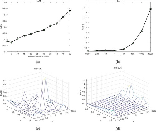
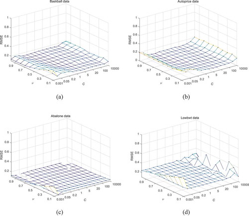
To analyze this phenomenon, four more data sets (Baskball, Autoprice, Abalone, and Lowbwt) are selected to run different combinations of parameters, as shown in Figure 2. For both these data sets, we can confirm that nu-ELR performs smoother on local parameter combinations (ν, C) of (0.1–1, 0.1–100) than the whole combinations. For (d) of Figure 2, if we fix the regularization parameter C at some value and vary the parameter ν in a large range, we found that generalization performance of nu-ELR is less sensitive to the variation of parameter ν.

Figure 2. Generalization performance of nu-ELR on four data sets. (a) Baskball, (b) Autoprice, (c) Abalone, (d) Lowbwt.

Statlib Data Sets

In this section, the performance of four learning models is tested through experiments of Statlib data sets, which contain 15 benchmark data sets, as listed in Table 1.

Table 1. Statlib data sets.

	Data sets	# Training samples	# Testing samples	# attributes
1	Bodyfat	130	122	14
2	Balloon	1000	1001	2
3	Baskball	50	46	4
4	Bolts	20	20	7
5	Elusage	25	20	2
6	fruitfly	60	65	4
7	lowbwt	100	89	9
8	Gascons	15	13	4
9	Mbagrade	30	31	2
10	Pollution	30	30	15
11	Quake	1000	1178	3
12	Sensory	300	276	11
13	Strike	300	325	6
14	Space-ga	1500	1607	6
15	Veteran	70	67	7

In our experiments, for each evaluated learning model, we use one training/testing partition to do parameter selection. Once the parameter selection process is completed, the selected model is used for other partitions. The selected parameter combination is then used for all independent trials, and the training and testing samples are randomly selected for each trial. First of all, we report model selection results for both four learning models, the selected combinations of parameters are listed in Table 2.

Table 2. Parameters setting on Statlib data sets.

Data set	ELM$L$	ELR$C$	nu-SVR$\left(\nu ,\gamma \right)$	nu-ELR$\left(\nu ,C\right)$
Bodyfat	20	0.1	(0.8,5)	(0.5,100)
Balloon	10	1	(0.1,5)	(0.6,1000)
Baskball	10	0.01	(0.5,10)	(0.5,100)
Bolts	5	0.1	(0.4,5)	(0.6,2)
Elusage	5	1000	(0.1,2)	(0.2,50)
fruitfly	5	0.1	(0.7,5)	(0.2,0.01)
lowbwt	10	0.01	(0.1,1)	(0.5,1)
Gascons	5	0.1	(0.1,1)	(0.2,10)
Mbagrade	5	10	(0.8,2)	(0.6,0.5)
Pollution	10	0.01	(0.3,10)	(0.6,1)
Quake	20	100	(0.3,1000)	(0.5,1)
Sensory	5	0.001	(0.3, 0.001)	(0.3,0.1)
Strike	5	0.001	(0.3, 0.01)	(0.2, 1)
Space-ga	10	0.1	(0.5, 1)	(0.2, 1000)
Veteran	5	0.1	(0.2, 0.2)	(0.4, 0.2)

For both 15 data sets, 50 trials have been conducted for each dataset. Experimental results include the root-mean-square error (RMSE) and the training time (s), as shown in Tables 3 and 4. For 11 out of 15 data sets, nu-ELR gives the best performance of RMSE. We also see that nu-ELR achieves the second-best performance for four other data sets when compared with three learning models. Clearly, nu-ELR performs better than ELR for all 15 data sets. Another observation is worth noting. It can be seen that for Balloon, Mbagrade, Space-ga data sets, compared to other learning models, nu-SVR performs significantly worse. A possible explanation is that the generalization performance of nu-SVR is very sensitive to the model parameters. After parameter selection, even nu-SVR performs well on one training/testing partition, it may perform very bad on other partitions.

Table 3. Performance comparison of four learning models (RMSE) on Statlib data sets.

Data sets	ELM	ELR	nu-SVR	nu-ELR
Bodyfat	0.0313	0.0219	0.0233	0.0209
Balloon	0.0075	0.0092	0.3464	0.0087
Baskball	0.1401	0.1329	0.1313	0.1300
Bolts	0.2571	0.1524	0.1998	0.1442
Elusage	0.1371	0.1549	0.2466	0.1391
fruitfly	0.2005	0.1985	0.2034	0.1929
lowbwt	0.1113	0.1062	0.1262	0.1025
Gascons	0.0861	0.0816	0.0518	0.0696
Mbagrade	0.2350	0.2167	0.4103	0.2164
Pollution	0.1616	0.1291	0.1404	0.1247
Quake	0.1735	0.1813	0.2316	0.1739
Sensory	0.1651	0.1645	0.1648	0.1643
Strike	0.0780	0.0791	0.0819	0.0733
Space-ga	0.0394	0.0389	0.1657	0.0369
Veteran	0.1583	0.1552	0.1572	0.1543

Table 4. Training time comparison of four learning models (s) on Statlib data sets.

Data sets	ELM	ELR	nu-SVR	nu-ELR
Bodyfat	7.1439e-04	0.0940	0.1234	0.0917
Balloon	7.3773e-04	24.0715	30.667	5.2424
Baskball	4.9741e-04	0.0280	0.0217	0.0268
Bolts	4.5620e-04	0.0106	0.0165	0.0113
Elusage	2.7205e-04	0.0110	0.0193	0.0083
fruitfly	2.8080e-04	0.0242	0.2113	0.0088
lowbwt	4.7517e-04	0.0481	0.4072	0.0382
Gascons	2.1406e-04	0.0090	0.0035	0.0072
Mbagrade	3.5045e-04	0.0149	0.1081	0.0057
Pollution	2.2938e-04	0.0100	0.0103	0.0174
Quake	0.0016	25.3534	1.1842	3.3344
Sensory	4.6532e-04	0.3414	0.2442	0.0626
Strike	4.2776e-04	0.4175	0.1477	0.0648
Space-ga	8.1541e-04	81.2082	14.1243	7.1489
Veteran	3.7889e-04	0.0244	0.0294	0.0177

The training time experiment (see Table 4) shows that the advantage of the ELM is quite obvious, as iteration is no need in the ELM training process. The training time of three learning models is similar to each other, except nu-SVR on some data sets (Balloon, Mbagrade, Space-ga). This phenomenon is originated from the fact that nu-SVR hardly finds the global solution within the limited iterations.

UCI Data Sets

In this section, the performance of four learning models is tested through experiments of UCI data sets, which contain 11 benchmark data sets, as listed in Table 5. Table 6 shows the model selection results.

Table 5. UCI data sets.

	Data sets	# Training samples	# Testing samples	# attributes
1	Abalone	2000	2177	8
2	Autoprice	80	79	15
3	Cleveland	150	153	13
4	Cloud	50	58	9
5	Housing	250	256	13
6	Machine_cpu	100	109	36
7	Mpg	200	192	7
8	Pyrim	40	34	27
9	Servo	80	87	19
10	triazines	90	96	58
11	Mg	700	685	6

Table 6. Parameters setting on UCI data sets.

Data sets	ELM$L$	ELR$C$	nu-SVR$\left(\nu ,\gamma \right)$	nu-ELR$\left(\nu ,C\right)$
Abalone	10	10	(0.1,5)	(0.4,10000)
Autoprice	20	0.01	(0.4,0.1)	(0.6,100)
Cleveland	20	0.1	(0.5,10)	(0.5,1)
Cloud	10	0.1	(0.5,5)	(0.6,10)
Housing	50	0.01	(0.5,2)	(0.2,1000)
Machine_cpu	10	10	(0.3,2)	(0.2,2)
Mpg	20	1	(0.5,1)	(0.7,1000)
Pyrim	10	0.001	(0.6,1)	(0.8,0.5)
Servo	20	0.1	(0.2,1)	(0.8,20)
triazines	10	0.01	(0.4,0.5)	(0.4,2)
Mg	10	1	(0.3,1)	(0.6,100)

From Table 7, out of 11 data sets, nu-ELR performs the best on 7 data sets, while nu-SVR performs the best on 4 other data sets. For Machine_cpu data set, we see that original nu-SVR is significantly better than other learning models when compared with RMSE. The most likely explanation for the superior performance of nu-SVR is that this data set is not sensitive to different training/testing partitions. For the Mpg dataset, it is worth noting that nu-SVR performs very badly compared to three other learning models, which has been discussed above. Table 8 gives the training time comparison. An interesting point of comparison is with the Mpg data set. Although nu-SVR performs very badly, less training time is need compared to ELR and nu-ELR.

Table 7. Performance comparison of four learning models (RMSE) on UCI data sets.

Data sets	ELM	ELR	nu-SVR	nu-ELR
Abalone	0.0803	0.0788	0.1239	0.0785
Autoprice	0.1024	0.0916	0.1361	0.0913
Cleveland	0.2279	0.2250	0.2158	0.2173
Cloud	0.0852	0.0731	0.0733	0.0729
Housing	0.0963	0.0837	0.0872	0.0826
Machine_cpu	0.1089	0.0638	0.0397	0.0629
Mpg	0.0789	0.0760	0.4228	0.0746
Pyrim	0.1616	0.1120	0.1097	0.1108
Servo	0.1363	0.1062	0.1139	0.0967
triazines	0.2007	0.1859	0.1961	0.1850
Mg	0.1738	0.1723	0.1658	0.1682

Table 8. Training time comparison of four learning models (s) on UCI data sets.

Data set	ELM	ELR	nu-SVR	nu-ELR
Abalone	4.8428e-04	3.6564	6.3009	0.3711
Autoprice	5.4263e-04	0.0433	0.0393	0.0376
Cleveland	4.4052e-04	0.1024	0.0317	0.0506
Cloud	3.6650e-04	0.0374	0.0241	0.0273
Housing	0.0012	0.4195	0.1272	0.0761
Machine_cpu	4.1463e-04	0.0527	0.0277	0.0155
Mpg	6.5349e-04	0.1734	0.0828	0.1277
Pyrim	5.2440e-04	0.0188	0.0148	0.0179
Servo	4.1062e-04	0.0592	0.0344	0.0142
triazines	4.4782e-04	0.0364	0.0377	0.0322
Mg	3.2492e-04	0.0278	0.0265	0.0286

A Performance Evaluation of Kernel Methods

Obviously, the kernel $K_{\mathrm{E}\mathrm{L}\mathrm{M}}\left(x_i,x\right)$ plays an important role in determining the characteristics of the nu-ELR learning model and choosing different kernels may result in different performances. In this section, another experiment was set up to see how the kernel affects the performance of different data sets for nu-ELR. Four commonly used kernel functions of ELM kernel $K_{\mathrm{E}\mathrm{L}\mathrm{M}}(\mathbf{x},{\mathbf{x}}_s)=[G({\mathbf{a}}_1,b_1,\mathbf{x}),...,G({\mathbf{a}}_L,b_L,\mathbf{x}){]}^{\mathrm{T}}\cdot [G({\mathbf{a}}_1,b_1,{\mathbf{x}}_s),...,G({\mathbf{a}}_L,b_L,{\mathbf{x}}_s){]}^{\mathrm{T}}$ in literatures are adopted in this experiment:

• Sigmoid function:

$G(\mathbf{a},b,\mathbf{x})=1/(1+exp(-(\mathbf{a}\cdot \mathbf{x}+b)))$

• Sin function:

$G(\mathbf{a},b,\mathbf{x})=sin(\mathbf{a}\cdot \mathbf{x}+b)$

• Hard-limit function:

$G(\mathbf{a},b,\mathbf{x})=\mathrm{h}\mathrm{a}\mathrm{r}\mathrm{d}\mathrm{l}\mathrm{i}\mathrm{m}\mathrm{i}\mathrm{t}(\mathbf{a}\cdot \mathbf{x}+b)$

• Exponential function:

$G(\mathbf{a},b,\mathbf{x})=\mathrm{e}\mathrm{x}\mathrm{p}(-(\mathbf{a}\cdot \mathbf{x}+b))$

All the vectors$\alpha$and variables $b$ in these kernel functions are set the same, which are randomly generated from (−1, 1)^N×(0, 1) based on the uniform probability distribution. The RMSE of regression performance on the test sets, across the Statlib data sets and UCI data sets, for the different nu-ELR kernels is shown in Tables 9 and 10.

Table 9. Comparison results of four kernel functions on Statlib data sets.

Data sets	Sin	Hard	Exp	Sigmoid
Bodyfat	0.0139	0.0380	0.0422	0.0084
Balloon	0.0093	0.1519	0.0063	0.0057
Baskball	0.1685	0.1826	0.1657	0.1559
Bolts	0.3475	0.3156	1.0543	0.1492
Elusage	0.1281	0.1319	0.1248	0.1424
fruitfly	0.1876	0.1826	0.1919	0.1842
lowbwt	0.2043	0.2808	0.3129	0.2373
Gascons	0.5156	0.3786	0.7419	0.2849
Mbagrade	0.2225	0.2314	0.2180	0.2110
Pollution	0.2283	0.1579	0.5764	0.1603
Quake	0.1693	0.1691	0.1693	0.1693
Sensory	0.1984	0.1720	0.2427	0.1512
Strike	0.0642	0.0695	0.0730	0.0564
Space-ga	0.0463	0.0702	0.0471	0.0395
Veteran	0.3758	0.2223	0.5527	0.1630

Table 10. Comparison results of four kernel functions on UCI data sets.

Data sets	Sin	Hard	Exp	Sigmoid
Abalone	0.1129	0.3151	0.1264	0.1059
Autoprice	0.2095	0.1072	0.2592	0.0991
Cleveland	0.2569	0.2480	0.3321	0.2241
Cloud	0.1343	0.1286	0.1643	0.0918
Housing	1.1795	0.2573	2.6837	0.1901
Machine_cpu	0.0600	0.0631	0.0386	0.0555
Mpg	0.2035	0.1444	0.2243	0.1060
Pyrim	0.0890	0.0827	0.1368	0.0939
Servo	0.0907	0.0950	0.1153	0.0875
triazines	0.2156	0.1893	0.4323	0.1936
Mg	0.1744	0.1679	0.1749	0.1769

From both two tables, we see that the Sigmoid kernel shows the best performance over most of the data sets. The Sin and Hard kernels show similar performance over more than half of all data sets. Hard kernel is the second most accurate in our experiments, but is clearly less accurate than Sigmoid kernel. As the computational cost of each kernel is very similar, the comparison of training time is not shown in this experiment.

Conclusions

By a simple reformulation of ELR with parameter nu, a novel ELR formulation is proposed in this work as an inequality-constrained minimization problem with the key advantage being the new parameter nu is only searched within the range [0, 1]. It is further proposed to solve the minimization problem using the active set algorithm. Experimental results on two different data repositories, including 26 regression problems, demonstrate that nu-ELR achieves the best performance over most of the regression problems, compared with ELM, ELR, and nu-SVR learning models. In particular, it provides a fair comparison on the RMSE of the different kernels of nu-ELR. It is clear from these results that some kernels are better than others, and certain kernels are better suited to certain types of problems. In future works, the proposed approach will be extended for other kernel-based learning methods.

Additional information

Funding

This work was supported by the Key Program of National Natural Science Foundation of China (91646204), and the Natural Science Foundation of Jiangsu (Grant No. BK20160148).

References

- Bartlett, P. L. 1998. The sample complexity of pattern classification with neural networks: The size of the weights is more important than the size of the network. IEEE Transactions on Information Theory 44 (2):525–36. doi:10.1109/18.661502.
- Blake, C. K., and C. J. Merz. 2013. UCI repository of machine learning databases. http://archive.ics.uci.edu/ml/.
- Bu, Z., J. Li, C. Zhang, J. Cao, A. Li, and Y. Shi. 2019. Graph K-means based on leader identification, dynamic game, and opinion dynamics. IEEE Transactions on Knowledge and Data Engineering. doi:10.1109/TKDE.2019.2903712.
- Chang, C. C., and C. J. Lin. 2002. Training v-support vector regression: theory and algorithms. Neural Computation 14 (8):1959–77. doi:10.1162/089976602760128081.
- Cortes, C., and V. Vapnik. 1995. Support vector networks. Machine Learning 20:273–97. doi:10.1007/BF00994018.
- Ding, S., N. Zhang, J. Zhang, X. Xu, Z. Shi. 2017. Unsupervised extreme learning machine with representational features. International Journal of Machine Learning and Cybernetics. 8(2):587–95. doi:10.1007/s13042-015-0351-8.
- Ding, X., and B. Chang. 2014. Active set strategy of optimized extreme learning machine. Chinese Science Bulletin 59 (31):4152–60. doi:10.1007/s11434-014-0512-2.
- Ding, X. J., Y. Lan, Z. F. Zhang, and X. Xu. 2017. Optimization extreme learning machine with ν regularization. Neurocomputing 261:11–19. doi:10.1016/j.neucom.2016.05.114.
- Fletcher, R. 1981. Practical Methods of Optimization: Volume2 Constrained Optimization. New York: Wiley.
- Frénay, B., and M. Verleysen. 2010. Using SVMs with randomized feature spaces: An extreme learning approach, in: Proceedings of The 18th European Symposium on Artificial Neural Networks (ESANN), Bruges, Belgium, 28–30 April, 2010, 315–20.
- Ghanty, P., S. Paul, and N. R. Pal. 2009. NEUROSVM: An architecture to reduce the effect of the choice of kernel on the performance of svm. Journal of Machine Learning Research 10:591–622.
- He, Q., J. Xin, C. Y. Du, F. Zhuang, Z. Shi. 2014. Clustering in extreme learning machine feature space. Neurocomputing 128:88–95. doi:10.1016/j.neucom.2012.12.063.
- Huang, G.-B., L. Chen, and C.-K. Siew. 2006. Universal approximation using incremental constructive feedforward networks with random hidden nodes. IEEE Transactions on Neural Networks 17 (4):879–92. doi:10.1109/TNN.2006.875977.
- Huang, G.-B., X. Ding, and H. Zhou. 2010. Optimization method based extreme learning machine for classification. Neurocomputing 74:155–63. doi:10.1016/j.neucom.2010.02.019.
- Huang, G.-B., H. Zhou, X. Ding, and R. Zhang. 2012. Extreme learning machine for regression and multiclass classification. IEEE Transaction on System, Man, and Cybernetics-Part B: Cybernetics 42 (2):513–29. doi:10.1109/TSMCB.2011.2168604.
- Huang, G.-B., Q.-Y. Zhu, K.-Z. Mao, C.-K. Siew, P. Saratchandran, and N. Sundararajan. 2006. Can threshold networks be trained directly? IEEE Transactions on Circuits and Systems-II: Express Briefs 53 (3):187–91. doi:10.1109/TCSII.2005.857540.
- Huang, G.-B., Q.-Y. Zhu, and C.-K. Siew. 2006. Extreme learning machine: Theory and applications. Neurocomputing 70:489–501. doi:10.1016/j.neucom.2005.12.126.
- Lauren, P., G. Qu, J. Yang, P. Watta, G-B. Huang, A. Lendasse. 2018. Generating word embeddings from an extreme learning machine for sentiment analysis and sequence labeling tasks. Cognitive Computation 10(4):625–38. doi:10.1007/s12559-018-9548-y.
- Mike, M. 2005. Statistical datasets. http://lib.stat.cmu.edu/datasets/.
- Park, J., and I. W. Sandberg. 1991. Universal approximation using radial basis-function networks. Neural Computation 3:246–57. doi:10.1162/neco.1991.3.2.246.
- Schölkopf, B., A. Smola, R. C. Williamson, and P. L. Bartlett. 2000. New support vector algorithms. Neural Computation 12:1207–45. doi:10.1162/089976600300015565.
- Shin, Y., and J. Ghosh. 1995. Ridge polynomial networks. IEEE Transactions on Neural Networks 6 (3):610–22. doi:10.1109/72.377967.
- Zhang, Q., and A. Benveniste. 1992. Wavelet networks. IEEE Transactions on Neural Networks 3 (6):889–98. doi:10.1109/72.165591.