Artificial Color Constancy via GoogLeNet with Angular Loss Function

ABSTRACT

Color constancy is the ability of the human visual system to perceive colors unchanged independently of illumination. Giving a machine this feature will be beneficial in many fields where chromatic information is used. Particularly, it significantly improves scene understanding and object recognition.In this article, we propose a transfer learning-based algorithm, which has two main features: accuracy higher than many state-of-the-art algorithms and simplicity of implementation. Despite the fact that GoogLeNet was used in the experiments, the given approach may be applied to any convolutional neural networks. Additionally, we discuss the design of a new loss function oriented specifically to this problem and propose a few of the most suitable options.

Introduction

Color is an important part of visual information. However, color is not an intrinsic feature of an object, but the result of interaction between scene illumination, object’s reflection, camera sensor’s sensitivity, etc. Since most applications require only the object’s intrinsic characteristics, separation of this information (particularly, removing illumination color casts) is an essential task.

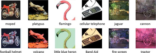
Human visual system solves this task via color constancy (CC) – a complex mechanism that involves color adaptation, color memory, and other features of human vision. Creation of an artificial algorithm that is able to do the same would be beneficial for many computer vision applications. Scene understanding, object recognition, pattern recognition, stereo vision, tracking, quality control, and many other fields use chromatic information and may suffer from its falseness. For example, Hosseini and Poovendran (Hosseini and Poovendran 2018) have illustrated how the VGG-16 network (Simonyan and Zisserman 2014) can be “fooled” by wrong colors (Figure 1).

Figure 1. Classification of images by VGG-16 net. Top row: original images from Caltech 101 dataset (Fei-Fei, Fergus, and Perona 2004); bottom row: the same images casted by random uniform illumination.

Despite the high importance of this problem, a universal solution still has not been found. Recently, the development of machine learning techniques and especially convolutional neural networks (CNNs) facilitated the creation of more accurate CC algorithms. Considering that a majority of original CNNs designed specifically for CC are quite simple and consist of only a few layers, we propose to improve their efficiency by means of more deep and more powerful nets using a transfer learning approach which is widely used in deep learning. Besides the gain in complexity, this approach allows us to greatly reduce training time and givespeople, who are not familiar with deep learning and cannot design CNN from scratch an opportunity to use efficient algorithms for their needs. (The shortest form of our algorithm is only 30 lines of code long and takes just a few hours to train.)

The general framework of CNN-based CC methods is an image regression that predicts coordinates of an illumination vector. Since the length of a vector is normalized in the result, only its orientation is important. Consequently, we propose, instead of mean squared error (MSE), which tries to fit both orientation and length, to use an angular loss function which considers only orientation of a vector and adds flexibility in parameters which are not important for the given task. The potential design of the angular loss function is not unique ; hence, we further discuss a few possible options for it.

Related Work

Methods of computational CC may be separated into two big groups: statistics based and learning ased. Methods from the first group were widely used in the last decades and exploit statistics of a single image. Moreover, in general, they usually apply strong empirical assumptions and operate in their limits. From these methods, we can highlight the most important ones: Gray World (Buchsbaum 1980), which is based on the assumption that average color in the image is gray and tries to estimate color of illumination as shift causing non-gray average; White Patch (Brainard and Wandell 1986), which is based on the assumption that the brightest point on image is a perfect white reflector and uses its color as color of illumination; Gray-Edge (Van de Weijer, Gevers, and Gijsenij 2007); and some more recent methods (Cheng, Prasad, and Brown 2014; Gao et al. 2014; Yang, Gao, and Li 2015). All of them were unified in a single framework by Van de Weijer, Gevers, and Gijsenij (2007).

Learning-based techniques estimate illumination color using a model created on a training dataset. In general, learning-based methods are shown to be more accurate than statistics-based approaches. This group includes a gamut mapping algorithm (Finlayson, Hordley, and Tastl 2003), an Support Vector Regression-based algorithm (Funt and Xiong 2004), an exemplar-based algorithm (Joze and Drew 2014), and numerous CNN-based algorithms presented in the last 3 years (Bianco, Cusano, and Schettini 2015a; Fourure et al. 2016; Hu, Wang, and Lin 2017; Lou et al. 2015; Shi, Loy, and Tang 2016). Many of the neural network-based algorithms (Cardei, Funt, and Barnard 2002; Cheng et al. 2015; Finlayson, Hordley, and Hubel 2001; Rosenberg, Hebert, and Thrun 2001) use hand-crafted, low-level visual features; however, most recent algorithms learn features using CNNs. Bianco, Cusano, and Schettini (2015a) first used patch-based CNNs for CC; in their work, simple CNN was used to extract local features which then were pooled (Bianco, Cusano, and Schettini 2015a) or passed to a support vector regressor (Bianco, Cusano, and Schettini 2015b). Later, Shi, Loy, and Tang (2016) proposed a more advanced network to deal with estimation ambiguities. The usage of the patches cropped from the images increases the size of the training dataset and augmentation of the data, however, at the cost of loss of semantic information. Algorithm of Lou et al. (2015) works with full images and processes them with deep CNN that was pretrained on a big ImageNet dataset with labels evaluated from hand-crafted CC algorithms and fine-tuned on each single dataset with ground-truth labels. This work is the most relevant to the algorithm presented in this paper but uses much simpler network as a base (AlexNet (Krizhevsky, Sutskever, and Hinton 2012), while we use GoogLeNet (Szegedy et al. 2015)) and does not prove the necessity of the first step (in this article, higher accuracy was achieved without using any hand-crafted labels). In the work of Fourure et al. (2016), custom mixed Max-Minkowski pooling and single max pooling networks were presented that demonstrated state-of-the-art accuracy. The latest and, to the best of our knowledge, the most accurate algorithm was presented by Hu, Wang, and Lin (2017) and is called FC⁴. FC⁴ is a fully convolutional network that allows using images without resizing or cropping; also, it uses confidence-weighed pooling which helps avoid ambiguity through assignment to each patch confidence weights according to the value they provide for CC estimation. Our algorithm, similar to the algorithm of Lou et al. (2015), is not fully convolutional. This disadvantage, however, is not critical, because it can be solved in just one preprocessing step (resizing) with some loss of semantic information. Additionally, using any fully convolutional net instead of GoogLeNet also solves this problem. In addition to the above, there are also a few more specifically oriented works, for instance, aimed at face regions (Bianco and Schettini 2012), texture classification (Bianco et al. 2017), or videos (Qian et al. 2017).

Experimental

Problem Formulation

Following the previous works, our goal was to estimate the color of illumination, noted as $e=\left(e_1,e_2,e_3\right)$, by the given RGB image, to be able to discard illumination color cast using the Von Kries (1970) diagonal transform:

(1) $\left[\begin{array}{c}{R}_c\\ G_c\\ B_c\end{array}\right]=\left[\begin{array}{ccc}{e_1}^{-1}& 0& 0\\ 0& {e_2}^{-1}& 0\\ 0& 0& {e_3}^{-1}\end{array}\right]\left[\begin{array}{c}R\\ G\\ B\end{array}\right],$(1)

where $\left(R_c,G_c,B_c\right)$ is the corrected color as it appears under canonical white illumination. While there can be multiple illuminants in a scene, this work is focused on the traditional problem of estimating a single global illumination color, e.g., $e\left(x,y\right)=e$. Since we are not interested in the change in global intensity of illumination, all the illumination vectors were normalized as follows:

(2) $e\leftarrow \sqrt{3}\frac{e}{∥e∥}$(2)

For comparison of predicted illumination vector ($\hat{e}$) and ground-truth data (e), angular error metric (Equation (3)(3) $\epsilon =arccos\left(\frac{⟨\hat{e},e⟩}{∥\hat{e}∥∥e∥}\right)$(3) ) is considered. This metric was first proposed by Hordley and Finlayson (Hordley and Finlayson 2004) and nowadays is a standard in this field.

(3) $\epsilon =arccos\left(\frac{⟨\hat{e},e⟩}{∥\hat{e}∥∥e∥}\right)$(3)

Network Architecture

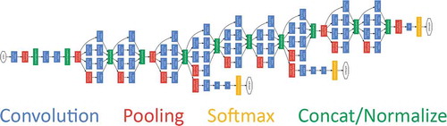
In the proposed approach, GoogLeNet by Szegedy et al. (2015) is used as a starting point for transfer learning. GoogLeNet is a 22-layer deep network (Figure 2) which achieved state-of-the-art accuracy in classification and detection in the ImageNet Large-Scale Visual Recognition Challenge 2014 (ILSVRC14). In comparison with AlexNet (Krizhevsky, Sutskever, and Hinton 2012), it uses 12× less parameters, therefore works faster and also provides higher accuracy. The core of this network is nine inception modules. The inception module basically acts as multiple convolution filters, which are applied to the same input, with some pooling. The results are then concatenated. This allows the model to take advantage of multilevel feature extraction and to cover a bigger area, while keeping a fine resolution for small information on the images.

Figure 2. Schematic representation of the GoogLeNet. Credits (Szegedy et al. 2015).

GoogLeNet has been trained on over a million images and can classify images into 1000 object categories. To modify the network for regression task, first of all, we had to remove the last three layers, which contain information on how to combine the features that the network extracts into class probabilities and labels (“FC,” “SoftmaxActivation,” “Softmax2”). In their place, a fully connected layer with three neurons and a regression output layer were added.

Angular Loss Function

The MSE loss function is used in the regression layer by default. When using it, the model is trying to predict the illumination coordinates as close as possible to the ground-truth data, e.g., predict the same vector. However, since lengths are normalized and only angles are important for CC task, we can benefit from it by removing restrictions on a length and adding a degree of freedom. Thus, by changing the loss function to the one which depends only on angle, we make the model more flexible and task oriented.

The primary value that the algorithm computes is a cosine of the angle between predicted values and ground truth. Considering this fact, the following loss functions were proposed:

(4) $L_1=arccoscos\epsilon =\epsilon$(4)

(5) $L_2=1-cos\epsilon$(5)

(6) $L_3=1-{cos}^2\epsilon ={sin}^2\epsilon$(6)

(7) $L_4=\sqrt{1-{cos}^2\epsilon }=sin\epsilon$(7)

Of course, choice is not limited to these options, but these are the simplest ones. To the best of our knowledge, only the $L_1$ function was used for CC by Hu, Wang, and Lin (2017), and $L_2$ was used by Hara, Vemulapalli, and Chellappa (2017) for a very different task. In the selection, we took into consideration the complexity of the function, its derivative, shape of the curve, and possible problematic points. Consequently, function $L_4$ was immediately discarded due to the complexity, complexity of the derivative, and the same behavior in the neighborhood of a 0 as $L_1$. Function $L_1$ is the most direct loss with respect to the error, and it also showed a good result in the case of FC⁴ net. However, the fact that the error is computed as arccosine of cosine makes the derivative much more complex (Equation (8)(8) $\begin{array}{rl}& \frac{\mathrm{\partial }{L}_1}{\mathrm{\partial }{\hat{e}}_i}=\frac{\mathrm{\partial }\left(arccoscos\epsilon \right)}{\mathrm{\partial }{\hat{e}}_i}=-\frac{1}{\sqrt{1-{cos}^2\epsilon }}\cdot \frac{\mathrm{\partial }\left(\frac{\hat{e},e}{∥\hat{e}∥∥e∥}\right)}{\mathrm{\partial }{\hat{e}}_i}=\\ & =\frac{1}{\sqrt{1-\frac{⟨\hat{e},e^2⟩}{{∥\hat{e}∥}^2{∥e∥}^2}}}\cdot \frac{{\hat{e}}_i⟨\hat{e},e⟩-e_i⟨e,e⟩}{{∥\hat{e}∥}^3\cdot ∥e∥}=\frac{{\hat{e}}_i⟨\hat{e},e⟩-e_i⟨e,e⟩}{\hat{e},\hat{e}\sqrt{\hat{e},\hat{e}⟨e,e⟩-{⟨\hat{e},e⟩}^2}}\end{array}$(8) ) and generates an error or NaN values when $\epsilon$ equals 0, π, 2π, … (that was a major problem in our experiment).

(8) $\begin{array}{rl}& \frac{\mathrm{\partial }{L}_1}{\mathrm{\partial }{\hat{e}}_i}=\frac{\mathrm{\partial }\left(arccoscos\epsilon \right)}{\mathrm{\partial }{\hat{e}}_i}=-\frac{1}{\sqrt{1-{cos}^2\epsilon }}\cdot \frac{\mathrm{\partial }\left(\frac{\hat{e},e}{∥\hat{e}∥∥e∥}\right)}{\mathrm{\partial }{\hat{e}}_i}=\\ & =\frac{1}{\sqrt{1-\frac{⟨\hat{e},e^2⟩}{{∥\hat{e}∥}^2{∥e∥}^2}}}\cdot \frac{{\hat{e}}_i⟨\hat{e},e⟩-e_i⟨e,e⟩}{{∥\hat{e}∥}^3\cdot ∥e∥}=\frac{{\hat{e}}_i⟨\hat{e},e⟩-e_i⟨e,e⟩}{\hat{e},\hat{e}\sqrt{\hat{e},\hat{e}⟨e,e⟩-{⟨\hat{e},e⟩}^2}}\end{array}$(8)

The expansion of the functions $L_2$ and $L_3$ in the Maclaurin series (Equations (9(9) $1-cos\epsilon =\frac{{\epsilon }^2}{2}+\frac{{\epsilon }^4}{24}-\frac{{\epsilon }^6}{720}+O\left({\epsilon }^8\right)=1-\sum _{k=1}^{\mathrm{\infty }}\frac{{\left(-1\right)}^k{\epsilon }^{2k}}{\left(2k\right)!}$(9) , 10)(10) $1-{cos}^2\epsilon ={\epsilon }^2-\frac{{\epsilon }^4}{3}+\frac{2{\epsilon }^6}{45}-\frac{{\epsilon }^8}{315}+O\left({\epsilon }^{10}\right)=-\sum _{k=1}^{\mathrm{\infty }}\frac{{\left(-1\right)}^k\left(2^{-1+2k}{\epsilon }^{2k}\right)}{\left(2k\right)!}$(10) ) clearly demonstrates their behavior proportional to ${\epsilon }^2$ around 0. We consider this feature beneficial for gradient computation by analogy with MSE loss.

(9) $1-cos\epsilon =\frac{{\epsilon }^2}{2}+\frac{{\epsilon }^4}{24}-\frac{{\epsilon }^6}{720}+O\left({\epsilon }^8\right)=1-\sum _{k=1}^{\mathrm{\infty }}\frac{{\left(-1\right)}^k{\epsilon }^{2k}}{\left(2k\right)!}$(9)

(10) $1-{cos}^2\epsilon ={\epsilon }^2-\frac{{\epsilon }^4}{3}+\frac{2{\epsilon }^6}{45}-\frac{{\epsilon }^8}{315}+O\left({\epsilon }^{10}\right)=-\sum _{k=1}^{\mathrm{\infty }}\frac{{\left(-1\right)}^k\left(2^{-1+2k}{\epsilon }^{2k}\right)}{\left(2k\right)!}$(10)

Additional analysis of their plots (Figure 3) reveals significant drawback of function $L_3$ – possibility to obtain an error of 180 degrees and negative values of illumination.

Figure 3. Plots of $y=1-cos\epsilon$ (solid line) and $y=1-{cos}^2\epsilon$ (dashed line).

Thereafter, loss function $L_2=1-cos\epsilon$ was used in our experiments. A potential issue that derivative will become zero at point π exists, but the probability of it is extremely low. Ultimately, derivatives of the functions $L_2$ and $L_3$ are given as follows:

(11) $\frac{\mathrm{\partial }{L}_2}{\mathrm{\partial }{\hat{e}}_i}=\frac{\mathrm{\partial }\left(1-cos\epsilon \right)}{\mathrm{\partial }{\hat{e}}_i}=-\frac{\mathrm{\partial }\left(\frac{⟨\hat{e},e⟩}{∥\hat{e}∥∥e∥}\right)}{\mathrm{\partial }{\hat{e}}_i}=\frac{{\hat{e}}_i⟨\hat{e},e⟩-e_i⟨e,e⟩}{{∥\hat{e}∥}^3\cdot ∥e∥}$(11)

(12)

Image Datasets

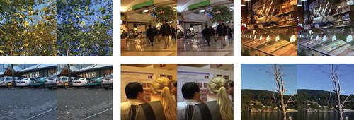
Two standard benchmark datasets, SFU Grayball (Ciurea and Funt 2003) and ColorChecker Reprocessed (other names: RAW dataset, 568-dataset, Gehler’s dataset) (Gehler et al. 2008; Lynch, Drew, and Finlayson 2013), are used. The Grayball dataset contains 11,346 real-world images. In each image, a gray ball is placed in the right-bottom of the image that allows to obtain the ground-truth illumination color. During training and testing, the gray ball has been removed from the image. The ColorChecker dataset contains 568 real-world images. The Macbeth ColorChecker chart is included in every scene acquired; thus, ground-truth illumination is known. In both training and testing subsets, ColorChecker chart has been removed.

Additionally, geometrical data augmentation was applied to both datasets. It consisted of random translations along the X- and Y-axis up to 30 pixels and horizontal reflections. The augmentation increases the variance of training data and helps to prevent the network from overfitting and memorizing the exact details of the training images. Particularly for CC task, models greatly benefit from chromatic augmentation, e.g., casting the images with semirandom illumination and changing corresponding ground-truth vectors. In this article, it was not used, but we imply that the accuracy of the presented algorithms may be increased using this technique (Fourure et al. 2016; Hu, Wang, and Lin 2017; Lou et al. 2015).

The fact that the proposed model contains a fully connected layer imposes a restriction on the size of the input image of 224 × 224 pixels. Hence, all the images were resized, and central square areas were cropped.

Other Experimental Details

All the models have been implemented in MATLAB 2017b, using Neural Network Toolbox. The simplicity and readability of MATLAB code allow creating and directly using models like ours for a wide range of audience, which we consider as an undoubted advantage. The source code is openly accessible and can be downloaded by the following link: https://github.com/acecreamu/color-constancy-googlenet. Notwithstanding the fact that the development of the algorithm and growth of its complexity have no limits, the simplest pure form of the given algorithm can fit in 30 lines of code.

The technological equipment used in the experiments consisted of only one laptop with Intel i7-7500U (2.7 GHz) CPU, 16 Gb RAM, and NVIDIA 950MX (2 Gb) GPU, which also supports the concept of the wide availability of presented methods.

Results

Following the previous papers, a 15-fold cross-validation was used for Grayball (Ciurea and Funt 2003) dataset. For much smaller ColorChecker (Gehler et al. 2008) dataset, only a threefold cross-validation was used in order to repeat the conditions of previous experiments and compare the results objectively. Each time, the corresponding dataset was partitioned into 15 or 3 subsets, and in a loop, each of them was used as a test set; after that the results of all the iterations were averaged. Such an approach provides a reliable evaluation of the model’s performance minimizing the influence of randomness.

Tables 1 and 2 present the comparison of our results with current state-of-the-art algorithms. Several standard metrics are reported in terms of angular error in degrees: mean, median, trimean or standard deviation, mean of the lowest 25% of errors, mean of the highest 25% of errors, and 95th percentile. For reasons unknown, very limited statistical data were reported in the case of Grayball dataset; however, there is no such problem in the case of ColorChecker dataset.

Table 1. The results obtained on SFU Grayball dataset, and comparison with state-of-the-art methods. First two sections correspond to statistic-based and learning-based methods.

	Mean	Median	Standard Deviation	Best 25%	Worst 25%	95th Percentile
Gray World, Buchsbaum (1980)	7.9	7.0	-	-	15.2	-
White Patch, Brainard and Wandell (1986)	6.8	5.3	-	-	-	-
Shades-of-Gray, Finlayson and Trezzi (2004)	6.1	5.3	-	-	-	-
2nd-order Gray-Edge, Van de Weijer, Gevers, and Gijsenij (2007)	6.1	4.3	-	-	-	-
Gray Patches, Yang, Gao, and Li (2015)	6.1	4.6	-	1.1	13.6	-
Local Surface Refl. Gao et al. (2014)	6.0	5.1	-	-	11.9	-
1st-order-Gray-Edge, Van de Weijer, Gevers, and Gijsenij (2007)	5.9	4.7	-	-	-	-
3D Scene Geometry, Elfiky et al. (2014)	5.4	4.5	-	-	-	-
Temporal sequence, Prinet, Lischinski, and Werman (2013)	5.4	4.6	-	-	-	-
Single max pooling, Fourure et al. (2016)	5.2	4.5	-	-	-	-
Mixed MaxL (Bianco, Cusano, and Schettini 2015b) pooling, Fourure et al. (2016)	4.9	4.3	-	-	-	-
Exemplar-based, Joze and Drew (2014)	4.4	3.3	-	-	-	-
AlexNet Retrained, Lou et al. (2015)	3.9	3.0	3.3	-	-	-
GoogLeNet + MSE	2.55	1.91	2.19	0.58	5.59	6.78
GoogLeNet + angular loss	1.98	1.49	1.87	0.39	4.51	5.73

Table 2. The results obtained on reprocessed ColorChecker dataset, and comparison with state-of-the-art methods. First two sections correspond to statistic-based and learning-based methods.

	Mean	Median	Trimean	Best 25%	Worst 25%	95th Percentile
White Patch, Brainard and Wandell (1986)	7.55	5.68	6.35	1.45	16.12	-
Edge-based Gamut, Barnard (2000)	6.52	5.04	5.43	1.90	13.58	-
Gray World, Buchsbaum (1980)	6.36	6.28	6.28	2.33	10.58	11.3
Second-order Gray-Edge, Van de Weijer, Gevers, and Gijsenij (2007)	5.13	4.44	4.62	2.11	9.26	-
Shades-of-Gray, Finlayson and Trezzi (2004)	4.93	4.01	4.23	1.14	10.20	11.9
Pixel-based Gamut, Barnard (2000)	4.20	2.33	2.91	0.50	10.72	14.1
Natural Image Statistics, Gijsenij and Gevers (2011)	4.19	3.13	3.45	1.00	9.22	11.7
19 Edge Moments, Finlayson (2013)	2.80	2.00	-	-	-	6.90
Mixed MaxL (Bianco, Cusano, and Schettini 2015b) pooling, Fourure et al. (2016)	3.33	2.63	-	-	-	-
Single max pooling, Fourure et al. (2016)	3.31	2.59	-	-	-	-
Exemplar-based, Joze and Drew (2014)	3.10	2.30	-	-	-	-
AlexNet Retrained, Lou et al. (2015)	3.1	2.30	-	-	-	-
Patch-CNN, Bianco, Cusano, and Schettini (2015a)	2.63	1.98	-	-	-	-
CCC, Barron (2015)	1.95	1.22	1.38	0.35	4.76	5.85
DS-Net (HypNet+SelNet), Shi, Loy, and Tang (2016)	1.90	1.12	1.33	0.31	4.84	5.99
SqueezeNet-FC^4, Hu, Wang, and Lin (2017)	1.65	1.18	1.27	0.38	3.78	4.73
GoogLeNet + MSE	3.06	2.15	2.32	0.48	7.01	9.64
GoogLeNet + angular loss	2.55	1.69	1.92	0.39	6.03	6.7

Table 1 shows the results obtained on SFU Grayball dataset and the comparison of the results with state-of-the-art methods. The first two sections correspond to statistic-based and learning-based methods. The top five results are highlighted with shades of gray.

In the case of both datasets, the model with angular loss outperforms the one with MSE loss. The empirical comparison of the different angular loss functions and design on the new ones may be a subject for future research.

Table 2 shows the results obtained on the reprocessed ColorChecker dataset and the comparison of the results with state-of-the-art methods. The first two sections correspond to statistic-based and learning-based methods. The top five results are highlighted with shades of gray.

Visual evaluation of results can be done using the examples illustrated in Figure 4.

Figure 4. An example of images from Grayball dataset before (left) and after (right) removing illumination color cast using the algorithm presented in this paper.

*Figures are given separately

Conclusion

In this article, we proposed an approach that allows to easily create effective CC algorithm. The presented technique may be applied to any advanced CNN. We used GoogLeNet, and depending on the dataset obtained the best or comparable with the best accuracy. A significant advantage of our approach is that it requires neither high skills in machine learning nor expensive technical equipment, nor a long time, which makes it available to the general public.

Also, we discussed the design of angular loss function, which is an important question for any CC algorithm. As a result, we chose function $1-cos\epsilon$, where $\epsilon$ is an angular error, because of its simplicity, efficiency, and high suitability for this task. However, the discussion and empirical examination are not finished, which may be extended in future works.

References

- Barnard, K. Improvements to gamut mapping colour constancy algorithms. European Conference on Computer Vision. 2000, Berlin; pp. 390–403.
- Barron, J. T. Convolutional color constancy. International Conference on Computer Vision. 2015, Santiago; pp. 379–87.
- Bianco, S., C. Cusano, P. Napoletano, and R. Schettini. 2017. Improving CNN-based texture classification by color balancing. Journal of Imaging 3 (33). doi:10.3390/jimaging3030033.
- Bianco, S., C. Cusano, and R. Schettini Color constancy using CNNs. Computer Vision and Pattern Recognition Workshops. 2015a; pp. 81–89. doi:10.3389/fnbeh.2015.00081.
- Bianco, S., C. Cusano, and R. Schettini. 2015b. Single and multiple illuminant estimation using convolutional neural networks. ArXiv E-prints 1508.00998.
- Bianco, S., and R. Schettini. Color constancy using faces. In Computer vision and pattern recognition. 2012, Providence; pp. 65–72.
- Brainard, D. H., and B. A. Wandell. 1986. Analysis of the retinex theory of color vision. Journal of the Optical Society of America A 3 (10):1651–61. doi:10.1364/JOSAA.3.001651.
- Buchsbaum, G. 1980. A spatial processor model for object colour perception. Journal of the Franklin Institute 310 (1):1–26. doi:10.1016/0016-0032(80)90058-7.
- Cardei, V. C., B. Funt, and K. Barnard. 2002. Estimating the scene illumination chromaticity by using a neural network. Journal of the Optical Society of America A 19 (12):2374–86. doi:10.1364/JOSAA.19.002374.
- Cheng, D., D. K. Prasad, and M. S. Brown. 2014. Illuminant estimation for color constancy: Why spatial-domain methods work and the role of the color distribution. Journal of the Optical Society of America 31 (5):1049–58. doi:10.1364/JOSAA.31.001049.
- Cheng, D., B. Price, S. Cohen, and M. S. Brown. 2015. Effective learning-based illuminant estimation using simple features. In Computer vision and pattern recognition, 1000–08.
- Ciurea, F., and B. Funt A large image database for color constancy research. In Imaging Science and Technology Eleventh Color Imaging Conference. 2003, Scottsdale; pp. 160–64.
- Elfiky, N., T. Gevers, A. Gijsenij, and J. Gonzalez. 2014. Color constancy using 3D scene geometry derived from a single image. In IEEE Transactions on Image Processing 23 (9):3855–68. doi:10.1109/TIP.83.
- Fei-Fei, L., R. Fergus, and P. Perona. Learning generative visual models from few training examples: An incremental Bayesian approach tested on 101 object categories. In Computer vision and pattern recognition. 2004, Washington, DC; pp. 178–178.
- Finlayson, G., and E. Trezzi Shades of gray and colour constancy. Color Imaging Conference. 2004; pp. 37–41. doi:10.1080/13557850410001673987.
- Finlayson, G. D. Corrected-moment illuminant estimation. International Conference on Computer Vision. 2013, Sydney; pp. 1904–11.
- Finlayson, G. D., S. D. Hordley, and P. M. Hubel. 2001. Color by correlation: A simple, unifying framework for color constancy. IEEE Transactions on Pattern Analysis and Machine Intelligence 23 (11):1209–21. doi:10.1109/34.969113.
- Finlayson, G. D., S. D. Hordley, and I. Tastl Gamut constrained illuminant estimation. International Conference on Computer Vision. 2003; 2:792–99. doi:10.1038/nmat1018.
- Fourure, D., R. Emonet, E. Fromont, D. Muselet, A. Trémeau, and C. Wolf Mixed pooling neural networks for color constancy. IEEE International Conference on Image Processing. 2016.
- Funt, B., and W. Xiong. 2004. Estimating illumination chromaticity via support vector regression. In Color and Imaging Conference 50 (8):341–48.
- Gao, S., W. Han, K. Yang, C. Li, and Y. Li. 2014. Efficient color constancy with local surface reflectance statistics. In European Conference on Computer Vision 8690:158–73.
- Gehler, P. V., C. Rother, A. Blake, T. Minka, and T. Sharp. Bayesian color constancy revisited. In Computer vision and pattern recognition. 2008, Anchorage; pp. 1–8.
- Gijsenij, A., and T. Gevers. 2011. Color constancy using natural image statistics and scene semantics. IEEE Transactions on Pattern Analysis and Machine Intelligence 33 (4):687–98. doi:10.1109/TPAMI.2010.93.
- Hara, K., R. Vemulapalli, and R. Chellappa. 2017. Designing deep convolutional neural networks for continuous object orientation estimation. ArXiv E-prints 1702.01499.
- Hordley, S., and G. Finlayson Re-evaluating color constancy algorithms. International Conference on Pattern Recognition. 2004, Cambridge; pp. 76–79.
- Hosseini, H., and R. Poovendran. 2018. Semantic adversarial examples. ArXiv E-prints 1804.00499.
- Hu, Y., B. Wang, and S. Lin. FC^4: Fully convolutional color constancy with confidence-weighted pooling. In Computer vision and pattern recognition. 2017, Honolulu; pp. 330–39.
- Joze, H. R. V., and M. S. Drew. 2014. Exemplar-based color constancy and multiple illumination. IEEE Transactions on Pattern Analysis and Machine Intelligence 36 (5):860–73. doi:10.1109/TPAMI.2013.169.
- Krizhevsky, A., I. Sutskever, and G. E. Hinton. 2012. ImageNet classification with deep convolutional neural networks. International Conference on Neural Information Processing Systems 1:1097–105.
- Lou, Z., T. Gevers, N. Hu, and M. P. Lucassen Color constancy by deep learning. British Machine Vision Conference. 2015, Swansea.
- Lynch, S. E., M. S. Drew, and G. D. Finlayson. 2013. Colour constancy from both sides of the shadow edge. IEEE ICCV Workshops 1:899–906.
- Prinet, V., D. Lischinski, and M. Werman Illuminant chromaticity from image sequences. International Conference on Computer Vision. 2013, Sydney.
- Qian, Y., K. Chen, J. Nikkanen, J. K. Kämäräinen, and J. Matas Recurrent color constancy. International Conference on Computer Vision. 2017, Venice; pp. 5459–67.
- Rosenberg, C., M. Hebert, and S. Thrun Color constancy using kl-divergence. International Conference on Computer Vision. 2001, Vancouver; 1:239–46.
- Shi, W., C. C. Loy, and X. Tang Deep specialized network for illuminant estimation. European Conference on Computer Vision, 2016, Amsterdam; pp. 371–87.
- Simonyan, K., and A. Zisserman. 2014. Very deep convolutional networks for large-scale image recognition. ArXiv E-prints 1409.1556.
- Szegedy, C., W. Liu, Y. Jia, P. Sermanet, S. Reed, D. Anguelov, D. Erhan, V. Vanhoucke, and A. Rabinovich. Going deeper with convolutions. In Computer Vision and Pattern Recognition. 2015, Boston; pp. 1–9.
- Van de Weijer, J., T. Gevers, and A. Gijsenij. 2007. Edge-based color constancy. IEEE Transactions on Image Processing 16 (9):2207–14. doi:10.1109/TIP.2007.901808.
- Von Kries, J. 1970. Influence of adaptation on the effects produced by luminous stimuli. In sources of color science. In Handbook of stuff I care about, ed. D. L. MacAdam, 120–26. Cambridge, MA: MIT Press.
- Yang, K.-F., S.-B. Gao, and Y.-J. Li. Efficient illuminant estimation for color constancy using grey pixels. In Computer Vision and Pattern Recognition. 2015, Boston; pp. 2254–63.