Analysis of the Ebola Outbreak in 2014 and 2018 in West Africa and Congo by Using Artificial Adaptive Systems

ABSTRACT

In this manuscript the Ebola outbreaks in 2014 and 2018 have been studied. On March 23, 2014, the World Health Organization announced the beginning of the Ebola outbreak in West Africa. The initial location was in a forested area in the south eastern portion of Guinea. We used three different methods to determine the origin of the outbreak. The first was a suite of artificial adaptive systems called Topological Weighted Centroid which located the outbreak origin at Longitude: −10.5337, Latitude: 8.1517. This area is 64 km from Guekedou, Guinea. We also used a Dynamic Naive Bayesian/Dynamic Networks Block Algorithm. The Bayesian algorithm shows the main source of the Ebola outbreak at Kissidougou. Both of these methods revealed the outbreak started in the forested area southeast of Guinea. The distance between Guekedou and Kissidougou is about 69 km. Furthermore, we used an artificial neural network (ANN) called Selfie to predict the outbreak diffusion. The Ebola outbreak in May 2018 in Democratic Republic of Congo was not as widespread as the outbreak in 2014. The outbreak was effecting the health zones of Bikoro and Iboko, and Wangata in Congo. We have used an ANN algorithm and predicted the origin of the outbreak at (Longitude: 18.3046, Latitude: −0.6865) in the Equator about 20 km at North-West of Bikoro.

Introduction

The initial WHO epidemiologic investigation revealed the first (index) case was a 2-year-old child from Meliandou (a village in Gueckedou prefecture in Nzerekore region of southern Guinea), Longitude: −10.061, Latitude: 8.616. According to the initial investigation the child died on December 6, 2013 but a secondary investigation confirmed the death of a child at the end of December. After the death of the index case, the sister, mother, grandmother of the child and a nurse, became victims 2–5, died on December 29, 2013, December 13, 2013, January 1, 2014, and January 29, 2014, respectively. Evidently, the fourteenth patient, a health-care worker from Gueckedou, caused the spread of the virus to Macenta, Nzerekoré, and Kissidougou in February 2014. (Sylvain et al. 2014)

The World Health Organization (WHO) was alerted of the Ebola outbreak in Guinea on March 23, 2014. The Ministry of Health (MoH) of Guinea notified the WHO of the rapidly spreading Ebola outbreak in the forested area south eastern of Guinea with a total of 49 cases including 29 deaths by March 22, 2014. The Ebola cases reported were in Guekedou (Longitude: −10.1336, Latitude: 8.5674), Macenta (Longitude: −9.4710, Latitude: 8.5435), Nzerekore (Longitude: −8.8238889, Latitude: 7.7472) and Kissidougou districts (Longitude:-10.1000, Latitude: 9.1833) (WHO Ebola Response Team 2014).

The recent (May 2018) Ebola outbreak was reported by WHO. According to the WHO reports the confirmed cases were in Bikoro and Iboka health zones, and in Wangata, one of the three health zones of Mbandaka (Ebola Virus Disease 2018; Ebola virus disease-Democratic Republic of the Congo, Disease outbreak news 2018; Update on the Ebola outbreak in Democratic Republic of Congo, Medicines Sans Frontiers, Doctor without Borders, May 2018).

Different approaches have been used to study the Ebola outbreak such as artificial adaptive systems, a fixable spatiotemporal growth, and deterministic model, a Markov model to estimate the weekly average number of secondary cases and using Mirador to find the most informative clinical factors related to the Ebola virus Diseases (Buscema 2015; Clubri et al. 2016; Santermans et al. 2016; Wayne et al. 2015).

Three algorithms in this effort have been used to validate the final results. All of these algorithms have been developed by the Semeion research center. We used the Topological Weighted Centroid (TWC) algorithm to find the possible location of the outbreak’s origin and analyze the dynamics of disease spread. The TWC suite of algorithms is based on statistical thermodynamics. They have been tested in other cases such as the E-coli outbreak in Germany (Buscema et al., 2009; Buscema et al. 2009, 2013; Grossi, Buscema, and Jefferson 2009). The details and the new development in TWC algorithm with some applications also have been discussed in (Buscema, Massini, and Sacco 2017). The Dynamic Naive Bayesian/Dynamic Networks Block (DNB) Algorithm was used to find the cause and effect of the Ebola outbreak and it is published here for the first time. The Selfie ANN has been applied also for the first time in paper. The main purpose of using different algorithms is to justify the results of using different methods and test them on the Ebola outbreak data. The core of our analysis is based on the TWC method. We have divided the data into eight sets and we have shown the method is stable. We have obtained the same prediction for the origin of the outbreak from all eight sets and the results were near the place that was reported by WHO as the origin of the Ebola outbreak. In summary, we validated our analyses by

• comparing the results from three different algorithms (TWC, DNB, and ANN Selfie),

• using different TWC algorithms (TWCα, TWCβ, and TWCϒ),

• applying TWCα for eight different sets and

• comparing with the results with the origin that was reported by WHO.

Table 1 shows a summary of the outbreak over six West African countries. Our data were obtained from WHO, HealthMap, and The World Bank.

Table 1. Summary of outbreak over six West African countries.

	Liberia	Sierra Leone	Guinea	Nigeria	Mali	Senegal
Population	4.294E6	6.092E6	11.75E6	173.6E6	15.30E6	14.13E6
Area (Km^2)	96320	72180	245720	173600000	15300000	14130000
Density	44.58	84.40	47.82	190.61	12.54	73.39
Ebola Cases	7168	6599	2134	20	8	1
Deaths	3016	1398	1260	8	6	0
Death/Ebola	0.42	0.21	0.59	0.4	0.75	0
Ebola/Population	1.67E-3	1.11E-3	1.82E-4	1.15E-7	5.23E-7	7.08E-8
Ebola/Area	7.44E-2	9.14E-2	8.68E-3	2.2E-5	6.56E-6	5.19E-6
Deaths/Population	7.02E-4	2.29E-4	1.07E-4	4.61E-8	3.92E-7	0
Deaths/Area	3.13E-2	1.94E-2	5.13E-3	8.78E-6	4.92E-6	0

According to information from the WHO, Ebola started in Guinea but spread out mostly to Liberia and Sierra Leone.

The Ebola dataset from the HealthMap included 83 locations (Table 2) from western Africa monitored for a period of 32 weeks (from March 4 to October 4, 2014). The number of new Ebola-infected persons was recorded every week for each city. Notice that the number of confirmed cases in seven locations is zero. We consider any error in the data as noise that can occur with real data.

Table 2. The Ebola dataset from the HealthMap including 83 locations from western Africa monitored for a period of 32 weeks (from 4 March to 4 October 2014).

Location	Latitude	Longitude	No. of cases
Foret de Panel	14.3676	−14.4611	4
Tambacounda	13.8986	−13.3754	6
Boffa	10.1715	−14.0317	32
Conakry 1	9.5093	−13.7121	28
Conakry 2	9.5377	−13.6782	28
Conakry 3	9.5408	−13.6833	28
Tondon	10.2539	−13.4173	26
Telimele Prefecture	10.9258	−13.3299	18
Forecariah	9.4305	−13.0880	27
Dabola	10.7482	−11.1089	27
Faranah Prefecture	10.4375	−10.9422	29
Dinguiraye	11.2998	−10.7157	26
Kissidougou	9.1848	−10.0996	28
gueckedou 1	8.5666	−10.1334	28
gueckedou 2	8.5675	−10.1336	28
kerouane prefecture	9.2667	−9.0167	20
Macenta Prefecture	8.5440	−9.4709	30
Nzerekore 1	7.7564	−8.8179	28
Nzerekore 2	7.7331	−8.8336	28
Kambia	9.1177	−12.9164	26
Bombali District	9.3343	−12.2494	24
Port Loko	9.7662	−12.7838	26
Freetown 1	8.4900	−13.2341	24
Freetown 2	8.4838	−13.2299	24
Waterloo	8.3385	−13.0721	23
Moyamba	8.0003	−12.4894	24
Tonkolili	9.5927	−11.7950	23
Bo	8.0363	−11.6803	24
Kemena	7.8767	−11.1878	26
Daru	7.9923	−10.8407	29
Kailahun	8.2837	−10.5667	26
Koindu	8.4633	−10.3386	29
Buedu	8.2803	−10.3719	29
bopolu	7.1986	−10.3704	8
Bushrod Island	6.3669	−10.7833	16
District 3 1	6.2505	−9.7564	28
District 3 2	6.4335	−9.3422	28
Doe	6.7470	−8.7504	3
Foya	8.3670	−10.2169	28
Gbarnga	7.0030	−9.4729	27
Gbehlay-Geh	7.3024	−8.5310	26
Kakata	6.5000	−10.2501	26
Klay	6.6691	−10.8301	26
Kolahun	7.9172	−10.0012	28
Mambah-Kaba	6.2624	−10.3602	26
Monrovia 1	6.3112	−10.8047	16
Monrovia 2	6.2874	−10.7736	16
New kru town	6.3698	−10.7920	16
Porkpa	7.2406	−11.0192	26
Potupo	5.2111	−7.8859	22
Sapo National Park	5.3489	−8.6058	9
Suakoko	7.0055	−9.6683	26
Tapeta	6.4922	−8.8607	27
Tchien	5.9166	−8.0838	26
Tewor	7.0003	−11.2964	26
Todee	6.4992	−10.5003	26
Voinjama	8.4221	−9.7477	26
Enugu	6.4454	7.4977	8
Asaba	6.1978	6.7284	5
Calabar	4.9517	8.3220	0
Federal Cptal Territory	8.8518	7.1639	0
Ife	7.4670	4.5664	8
Ikputu Nsuru	5.4142	7.4896	0
Kaduna 1	10.3261	7.7482	9
Kaduna 2	9.6136	8.1245	0
Kano	11.5072	8.5014	0
Lagos Island	6.4532	3.3959	16
Lagos Lagoon	6.5836	3.7483	16
Oduaha	5.0286	6.6306	6
Port Harcourt	4.7776	7.0136	6
Rivers	4.7501	6.8316	0
Ughelli	5.5001	5.9999	0
Zaria	11.0669	7.7001	5
Boende 1	−0.0230	20.8582	6
Boende 2	−0.2802	20.8793	6
Boende Moke	−0.4391	20.7742	6
Djera	−0.3432	20.5450	6
Equateur	0.6169	18.8239	6
Lokola	−0.6585	20.5985	6
Maniema	−1.9759	25.0176	6
Watsi Kengo	−0.8398	20.5621	6
Kouremale	11.9500	−8.7833	27
Bankoumana	12.4215	−7.6074	27

Table 3 shows the locations and the number of cases of the recent Ebola outbreak in Democratic Republic of Congo in May 2018 (Ebola Virus Disease 2018). The recent outbreak was controlled quickly and it was not as widespread as the outbreak in 2014. This is the ninth Ebola outbreak in the last 40 years in Congo. The most recent outbreaks in Congo were in Likate district in May 2017 and in Boende in 2014. Most of the outbreaks occurred in isolated areas (Update on the Ebola outbreak in Democratic Republic of Congo, Medicines Sans Frontiers, Doctor without Borders, May 2018). The outbreak is reported in 10 locations. Some of those locations are very close to each other (Update on the Ebola outbreak in Democratic Republic of Congo, Medicines Sans Frontiers, Doctor without Borders, May 2018). We have used three coordinates that represent Wangata, Bikoro and Iboko heath zones according to WHO reports (Ebola virus disease-Democratic Republic of the Congo, Disease outbreak news 2018).

Table 3. The locations and the number of cases of the Ebola outbreak in Congo (May 2018).

Location	No. Cases
Wangata	10
Bikoro	6
Mohel I	1
Momboyo	1
Ikoko Impenge	12
Bokongo	1
Itipi	13
Mpangi	2
Wenga	1
Loongo	1

The Model

The approach we used was based on artificial adaptive systems. For this study, we used the Topological Weighted Centroid (TWC) suite of algorithms (Buscema et al., 2009; Buscema et al. 2009, 2013; Buscema, Massini, and Sacco 2017; Grossi, Buscema, and Jefferson 2009), Dynamic Naive Bayesian (DNB) Algorithm, and Selfie ANN.

Topological Weighted Centroid Algorithm

The Topological Weighted Centroid, whose theory and successful applications have been discussed in detail in our previous publications (Buscema et al., 2009; Buscema et al. 2009, 2013; Buscema, Massini, and Sacco 2017; Grossi, Buscema, and Jefferson 2009), was used to predict the origin and to analyze the spread of the recent Ebola outbreak. In this paper, we discuss TWC briefly. The foundation of this artificial neural system algorithm is statistical mechanics. We define the possible states of the system in terms of the locations (longitude and latitude) of the outbreak. For each state, we use the Boltzmann factor to define the probability of the state and then we are able to define the free energy and entropy of the system. Using the free energy and entropy we can then configure the state space giving us the possible source(s). From the source we then predict the possible spread. We define the system similar to a two-dimensional physical system that is a combination of several point masses, charges, or heat sources. The system is a finite two-dimensional discrete space with some active points (the outbreak points similar to the heat sources or charges in a physical system). The effect of the outbreak on all points of the discrete space is given by some scalar fields similar to the electric potential or temperature field in a physical system. Here, in some of our algorithms, only the location of the outbreak points are used and in some in addition to the outbreak points, the coordinates of all points on the discrete space are used. We use the longitude and latitude of the points in the region of interest as the two-dimensional coordinates. Three different TWC algorithms, TWCα, TWCβ, and TWCγ were used. The main differences between them stem from different definitions of the state of the system.

TWCα

The average location of the outbreak in the TWCα algorithm is measured according to the distance of the outbreak points from each other. The TWCα calculates the optimum value of $\alpha$ parameter. This optimal value of $\alpha$ is used to predict the coordinate of the origin of the outbreak $\left(TW{C}_x\left(\alpha \right),TW{C}_y\left(\alpha \right)\right)$. The coordinate is given in terms of latitude and longitude. The weighting factor is defined in a similar way as the Boltzmann factor in statistical thermodynamics and is given by

(1) $W_i\left(\alpha \right)=\frac{1}{N-1}\sum _{j=1,j\ne i}^N{e}^{-\frac{d_{i,j}}{D}\alpha }$(1)

where $N$ is the total number of outbreak points (states), $d_{i,j}$ can be the Euclidean distance between point $i$ and $j$ or a function of the Euclidean distance, $D=max\left(d_{i,j}\right)$ and $\alpha$ is a variable parameter $0\le \alpha <\mathrm{\infty }$ that will be discussed later. In equation (1) because of $i\ne j$, the summation is divided by $N-1$. In this analysis we have used a particular function of Euclidean distance for $d_{i,j}$ that is called meta distance or indirect distance (Buscema, Massini, and Sacco 2017). From a physics perspective $d_{i,j}$ can be interpreted as the potential energy associated with sources $i$ and $j$. The sum over all weighting factors is similar to the partition function in statistical thermodynamics and works as a normalizing factor of the probability. It is

(2) $Z\left(\alpha \right)=\sum _{i=1}^N{W}_i\left(\alpha \right)$(2)

The probability of being in state $i$ is given by

(3) $P_i\left(\alpha \right)=\frac{W_i\left(\alpha \right)}{Z\left(\alpha \right)}$(3)

The coordinates of TWCα are defined as

(4) $TW{C}_x\left(\alpha \right)=\sum _{i=1}^N{x}_i{P}_i\left(\alpha \right)$(4)

and

(5) $TW{C}_y\left(\alpha \right)=\sum _{i=1}^N{y}_i{P}_i\left(\alpha \right)$(5)

As $\alpha \to 0$ $TWC\left(\alpha \right)$ approaches the center of mass of the system. The free energy, $F\left(\alpha \right)$, and entropy (information) $S\left(\alpha \right)$, of the system are defined in a similar way as in statistical thermodynamics,

(6) $F\left(\alpha \right)=\frac{-lnZ\left(\alpha \right)}{\alpha }$(6)

and

(7) $S\left(\alpha \right)=-\sum _{i=1}^N{P}_i\left(\alpha \right)ln{P}_i\left(\alpha \right)$(7)

The optimal value of$\alpha ={\alpha }^{\ast }$ is given by optimizing the free energy and entropy of the system. As $\alpha$ increases from zero to ${\alpha }^{\ast }$ the distance between the $TWC\left(\alpha \right)$ and the center of the mass increases and when $\alpha$ exceeds ${\alpha }^{\ast }$ the distance between $TWC\left(\alpha \right)$ and the center of mass starts decreasing. Therefore $\alpha ={\alpha }^{\ast }$ is a turning point. As $\alpha$ changes from zero to ${\alpha }^{\ast }$ the $TWC\left(\alpha \right)$ point follows a path from the center of mass to $TWC\left({\alpha }^{\ast }\right)$. According to this algorithm the coordinate of the point of interest (the origin of the outbreak) is at $TW{C}_x\left({\alpha }^{\ast }\right)$ and $TW{C}_y\left({\alpha }^{\ast }\right)$.

TWCβ

From a physical perspective, the TWCα calculates the interaction of sources with each other, similar to the interaction of masses or charges on each other. Now we want to find out the effect of the sources on the space. Each source of the outbreak would be an outbreak potential in the space. The potential (possibility) of outbreak in the near points to the source should be larger than the farther points. In the physics terminology, the source distribution would create a field in the space, similar to the gravitational field. The TWCβ algorithm is the foundation of the scalar field which is discussed later. This scalar field has a similar perspective as the electric potential due to an electric charge distribution. In the TWCβ algorithm, we include the distance of all points to themselves, $d_{i,j}=0$. Since the effect of a source on the neighboring region should be the largest effect thus the weight corresponding to $d_{i,j}=0$ should be the largest weight.

This algorithm is similar to TWCα. In that algorithm the distance of the point to itself was not included so, to include the distance of the point to itself, the weighting factor from equation (1) is replaced by

(8) $W_i\left(\beta \right)=\frac{1}{N}\sum _{j=1}^N{e}^{-\frac{d_{i,j}}{D}\beta }$(8)

Equation (8) shows the weight increases as $d_{i,j}$ deceases and the largest weight is for $d_{i,j}=0$ as we expected.

The partition function and probability are defined in a manner similar to that of (2) and (3):

(9) $Z\left(\beta \right)=\sum _{i=1}^N{W}_i\left(\beta \right)$(9)

and

(10) $P_i\left(\beta \right)=\frac{W_i\left(\beta \right)}{Z\left(\beta \right)}$(10)

The coordinates of TWCβ are given by the equations similar to that of (4) and (5),

(11) $TW{C}_x\left(\beta \right)=\sum _{i=1}^N{x}_i{P}_i\left(\beta \right)$(11)

and

(12) $TW{C}_y\left(\beta \right)=\sum _{i=1}^N{y}_i{P}_i\left(\beta \right)$(12)

We also define the free energy and entropy similar to equations (6) and (7). We will find the optimal value of $\beta ={\beta }^{\ast }$ in a similar way as was shown for TWCα. The optimal value of $\beta ={\beta }^{\ast }$ will be used to determine the topological weighted scalar $\beta$ and $\gamma$ fields that will be discussed shortly.

TWCγ

The $TWC\left({\gamma }_i\left(t\right)\right)$ is an algorithm that obtains a set of points (trajectory) associated with each outbreak point at step $t$. The parameter ${\gamma }_i\left(t\right)$ is variable thus $TWC\left({\gamma }_i\left(t\right)\right)$ is a vector associated with each outbreak point and gives it a trajectory that starts from the $i$-th outbreak point and continues to an optimal value. The optimal value will be discussed later. In this case, we have a weighting factor that associates two points to each other. We follow a logic similar to that of (1) without summation over $j$ in the weighting factor.

(13) $W_{i,j}\left({\gamma }_i\left(t\right)\right)=e^{-\frac{d_{i,j}}{D}{\gamma }_i\left(t\right)}$(13)

The partition function is given by

(14) $Z_i\left({\gamma }_i\left(t\right)\right)=\sum _{j=1}^N{W}_{i,j}\left({\gamma }_i\left(t\right)\right)$(14)

and probability function for the dependence of point $i$ to point $j$ is given by

(15) $P_{i,j}\left({\gamma }_i\left(t\right)\right)=\frac{W_{i,j}\left({\gamma }_i\left(t\right)\right)}{Z_i\left({\gamma }_i\left(t\right)\right)}$(15)

The coordinates of the $i$-th $TWC\left({\gamma }_i\left(t\right)\right)$ at step $t$ are given by

(16) $TW{C}_{i,x}\left({\gamma }_i\left(t\right)\right)=\sum _{i=1}^N{x}_j{P}_{i,j}\left({\gamma }_i\left(t\right)\right)$(16)

and

(17) $TW{C}_{i,y}\left({\gamma }_i\left(t\right)\right)=\sum _{i=1}^N{y}_j{P}_{i,j}\left({\gamma }_i\left(t\right)\right)$(17)

The entropy (information) associated to the $i$-th outbreak point is given by

(18) $S_i\left({\gamma }_i\left(t\right)\right)=-\sum _{j=1}^N{P}_{i,j}\left({\gamma }_i\left(t\right)\right)ln\left(P_{i,j}\left({\gamma }_i\left(t\right)\right)\right)$(18)

The optimal or final value of ${\gamma }_i\left(t^{\ast }\right)={{\gamma }_i}^{\ast }$ is given by the following equilibrium condition

(19) ${\left.\frac{\mathrm{\partial }{S}_i\left({\gamma }_i\left(t\right)\right)}{\mathrm{\partial }{\gamma }_i\left(t\right)}\right|}_{{\gamma }_i\left(t\right)={{\gamma }_i}^{\ast }}=0$(19)

There are $NTWC\gamma$ points, where $N$ is the number of outbreak points. Basically $TWC\gamma$ transforms the outbreak points to new $TWC\gamma$ points. It maps the $i$-th outbreak point to point $TW{C}_i\left({\gamma }_i\left(t\right)\right)$ at step $t$. Since $TW{C}_i\left({\gamma }_i\left(t\right)\right)$ is the trajectory of the $i$-th outbreak point, we can say $TWC\gamma$ maps the $i$-th point along a trajectory. The coordinates of $TWC\gamma$ will be used for the topological weighted scalar γ field that will be discussed in the next section.

The Topological Weighted Scalar β and γ Fields

The effect of the outbreak on the space according to our approach is given by the scalar fields (Buscema et al., 2009; Buscema et al. 2009, 2013; Buscema, Massini, and Sacco 2017; Grossi, Buscema, and Jefferson 2009). The outbreak creates a scalar field similar to an electrical or gravitational scalar potential. We associate the field with the outbreak distribution and the distances of the points on the space to the outbreaks points. Suppose the two-dimensional discrete space is given by $M$ points and there are $N$ outbreak points. The Topological Weighted Scalar β Field, at a point $k$ is defined as

(20) $TWS{F}_k\left({\beta }^{\ast }\right)=\frac{1}{N}\sum _{j=1}^N{e}^{-\frac{q_{k,j}}{D}}{\beta }^{\ast }$(20)

where $1<k<M$, $D$ is the maximum Euclidean distance between the outbreaks points, and $q_{k,j}$ is the Euclidean distance between the $k$-th point on the discrete space and the $j$-th outbreak point. There are $M$ values of $TWS{F}_k\left({\beta }^{\ast }\right)$ for each point on the two-dimensional space.

The Topological Weighted Scalar $\gamma$ Field ($TWS{F}_{\gamma }$), at a point $k$ can be defined in a similar manner to that of the Topological Weighted Scalar β Field:

(21) $TWS{F}_{\gamma k}\left({\beta }^{\ast }\right)=\frac{1}{N}\sum _{j=1}^N{e}^{-\frac{r_{k,j}}{D}}{\beta }^{\ast }$(21)

where $r_{k,j}$ is the Euclidean distance between the $k$-th point and the $j$-th $TW{C}_j\left({\gamma }_j\left(t\right)\right)$ point at step $t$.

Dynamic Naive Bayesian/Dynamic Networks Block Algorithm

Dynamic Naive Bayesian/Dynamic Networks Block (DNB) is an algorithm to cluster the complex cause–effect relationships in a discrete dataset representing a multivariate temporal process.

The DNB algorithm is composed of three parts:

1. Equations to detect the local cause–effect relations between the variables in the temporal flow (see equation (22));

2. Equations to establish the global and prevalent cause–effect relations between the variables for the entire temporal multivariate process (see equations from (23) to (25));

3. Equations to select the most likelihood cause–effect relations between variables at different time scales (Multi-Scale Entropy – MSE) in order to cluster them and to project them in the direct graph, a sparse or connected graph (equations (26) and (27)).

The temporal correlation is given by

(22) $I_{k,k+1,i,j}^p=x_{k,i}^p.x_{k+1,j}^p$(22)

where $x_{k,i}^p$ is the $k$-th instance of the $i$-th variable from the $p$-th sample.

The average of the temporal correlation is given by

(23) $\overline{x_{i,j}^p}=\frac{1}{M}\sum _{k=1}^{M-1}{I}_{k,k+1,i,j}^p$(23)

where $M$ is the number of time steps. The temporal correlation variance is

(24) ${\sigma }_{i,j}^p=\frac{1}{M}\sum _k^{M-1}{\left(I_{k,k+1,i,j}^p-\overline{x_{i,j}^p}\right)}^2$(24)

The temporal correlation strength according to the probability function of $x$, $\mathrm{p}\left(x\right)$, is given by

(25) $s_{i,j}^p=\sum _k^{M-1}{I}_{k,k+1,i,j}^p\mathrm{p}\left(I_{k,k+1,i,j}^p\right)$(25)

The global temporal correlation at different time scales is given by

(26) $t_{i,j}=\sum _p^Q\left(\frac{s_{i,j}^p}{{\sum }_z^N{s}_{z,j}^p}\right)$(26)

where $N$ is the number of variables and $Q$ is the number of samples.

The maximum of global temporal correlation gives the greatest likelihood of “Cause j ” of “Effect $i$”:

(27) $C_j=\mathrm{a}\mathrm{r}\mathrm{g}\mathrm{m}\mathrm{a}\mathrm{x}{\left\{{\mathrm{t}}_{\mathrm{i},\mathrm{j}}\right\}}_{\mathrm{i}}$(27)

Selfie Artificial Neural Network

Selfie ANN is an algorithm able to estimate the perception that a set of entities have of space where they are located in. This estimation allows to predict the diffusion of a process, if the assigned entities represent a sample of the process itself.

Selfie algorithm learns the position of each Entity in relation to any other. In this way the position of each entity is learned in a collective and convergent modality by the other entities.

When a new point appears in a specific position, all the trained entities will try to modify the position of the new point in relation to the logic that they have previously learned (the Hyper Surface computed).

The data organization to implement (training and testing) Selfie ANN is:

Training:

The Dataset for training phase is given by

(28) $DB={\left\{Input,Output\right\}}_{n=1}^{N^2}$(28)

Each input vector is any possible combination of two entities, $i$ and $j$, with a total of $N^2$.

(29) $Inpu{t}_n=\left\{x_{n,i},y_{n,i},x_{n,j},y_{n,j}\right\}$(29)

and each output vector is given by

(30) $Outpu{t}_{n,i}=\left\{x{ }_{n,i}^{\prime },y{ }_{n,i}^{\prime }\right\}$(30)

where $i,j$ are assigned points indices (entities) and $n$ is the index of the input and the output vectors. Each output vector defines how a second entity $\left(j\right)$ estimates the position of the first entity$\left(i\right)$.

Testing:

input vector is given as following

(31) $Inpu{t}_p^n={\left\{x_{n,p},y_{n,p},x_{n,j},y_{n,j}\right\}}_{n=1}^N$(31)

where $p$ the index of a generic point. Each input vector defines how a second entity $\left(j\right)$ estimates the position of a generic point $\left(p\right)$.

The output for testing is given by

(32) $Outpu{t}_p=\left\{\frac{1}{N}\sum _{n=1}^{N}x{ }_{n,p}^{\prime },\frac{1}{N}\sum _{n=1}^{N}y{ }_{n,p}^{\prime }\right\}$(32)

Each output vector defines how all N entities estimate the position of a generic point $\left(p\right)$.

During the test phase we may have 3 typical cases:

Normal case 1: The new point has the same position as the trained entities: in this case the new position assigned to it will be similar to its original position (according to the training error).

Normal case 2: The new point has different coordinates from any of the trained entities: in this case the new position assigned to it will be different from its original position, in order to maximize the function learned.

Relevant case: The new point has different coordinates from any of the trained entities, but this time its position remains the same. Consequently, this new point belongs to the learned function more that the trained Entities.

All the new points with different coordinates from any of the trained entities and whose position remains unchanged during the test phase, have to be considered the hidden entities of the computed function.

These new points belong to the function more than the trained entities. Consequently, they have to be considered the kernel of the function itself. These points may consider the virtual future of the studied process.

Results

The main part of our analysis is related to 2014 Ebola outbreak. The recent outbreak (May 2018 in Congo) was not as widespread as the 2014 outbreak and it has a simpler dynamics.

Ebola Outbreak 2014

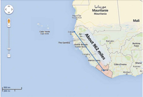
We have used the data provided by HealthMap. The longitude and latitude information for the outbreak location was not given. The longitude and latitude information was detained from Google Map. Figure 1 shows the map of Ebola outbreak as of September 1, 2014. Most of the Ebola cases are found in Liberia, Sierra Leone, and Guinea which are the neighboring countries. Figure 2 shows the scale of the Ebola outbreak over the countries with the most cases and shows an outbreak covering about 1000 miles (about 1600 km). We used “MapQuest Open” for mapping the results.

Figure 1. Ebola outbreak as September 1, 2014 from http://healthmap.org.

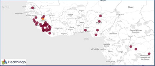
Figure 2. Estimated length over the area with the most outbreaks, Google. Map was used.

The outbreak is reported over 76 places (by removing seven places with zero outbreak from data given in Table 2) from March 2014 until the first week of October 2014 (32 weeks). We divided the data into eight sets, each set being 4 weeks (almost a month). Each set includes the data from the beginning (the first week) to the end of that set. For example, the data for set 5 is the data from the first week to the end of 20th week. We computed the coordinates of TWCα for different sets. The TWCα algorithm predicts the origin of the outbreak. The results are approximately the same and they are near the place that was reported by WHO as the origin of the Ebola outbreak. This can be considered as a self-validation techniques for TWC and testing the TWC with the real observation.

Table 4 shows the coordinates of TWCα for different sets. All of these results fall into the forested area in the south eastern part of Guinea. The distances between them are relatively small compared to the entire area of the Ebola outbreak in those countries. For example, the distance between TWCα of set 3 and set 7 is about 57 km which is the maximum distance between TWCα points. Guekedou (Longitude: −10.1336, Latitude: 8.5674) is the possible origin of the Ebola outbreak. The distances between the average TWCα and Guekedou is about 64 km. The distance has been calculated by using the “Latitude/Longitude Distance Calculator” that was obtained from the National Weather Service, National Hurricane Center.

Table 4. TWCα coordinates for dataset.

	Coordinate
	Longitude	Latitude	Number of infected places
Set 1	−10.3737	8.5369	6
Set 2	−10.3527	8.0220	40
Set 3	−10.7618	8.15169	48
Set 4	−10.7630	8.2119	50
Set 5	−10.7852	8.0741	56
Set 6	−10.7444	8.0514	58
Set 7	−10.2460	8.0719	74
Set 8	−10.2427	8.0940	76
Average	−10.5337	8.1517

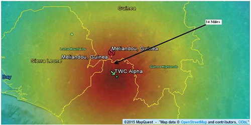
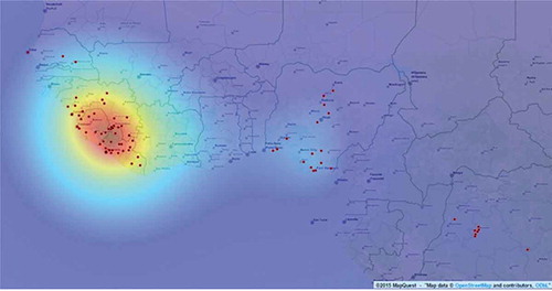
The TWCα algorithm estimates the original outbreak area. Figure 3 shows the estimated length corresponding to this area is about 34 miles (about 54 km). This result has been overlapped with the map of the region. The color map in Figure 3 represents the probability distribution for the possible origin of the outbreak through the region. The dark red shows the region with the highest probability of being the origin of the outbreak. It also shows the possible outbreak pattern in the region. The TWCβ and TWCγ give more information about the outbreak pattern.

Figure 3. The outbreak area predicted by the TWCα algorithm, open.mapquest was used.

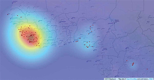
The scalar field from TWSFβ algorithm shows the prediction of the Ebola outbreak spread. The outbreak spread follows the gradient of the field. The TWSFβ scalar field was mapped onto the region in Figure 4. The hot spot is in the forested area in the south eastern portion of Guinea. The TWSFβ scalar field (Figure 4) not only shows the pattern of the outbreak around the origin similar to the results from the TWCα algorithm (Figure 3) but also captures two more regions (in the south of Nigeria and in the Democratic Republic of Congo). As we mentioned in the previous section, the weighting function in TWCβ includes the distance of a point from itself. This is the reason the additional regions have been captured in TWCβ algorithm. The main purpose of the TWCα algorithm is to find the location of the origin of the outbreak which was found at a distance of about 64 km from Guekedou. The new region(s) can be considered as the secondary region(s) of the outbreak and they can act independently in the outbreak distribution.

Figure 4. The TWSFβ scalar field for the Ebola outbreak. It captures three regions of outbreak, the main region which includes the origin of the outbreak (dark red) in the most west part of the map and two secondary regions in Nigeria and Democratic Republic of Congo (light blue). The red dots are the points of the dataset. Open.mapquest was used.

In Figure 5 the results of TWSFγ are shown. In this figure, we show the location of Guekedou, Macenta, Nzerekore, and Kissidougou districts. They are close to each other. Guekedou and Macenta are overlapping. According to the WHO, this is the origin of the Ebola outbreak (Sylvain et al. 2014; WHO Ebola Response Team 2014). The prediction of TWCγ matches the WHO report. The results from TWSFγ are very similar to the TWSFβ. The TWCγ algorithm follows the trajectory of the outbreak at each iteration step and finally gives the outbreak map at the optimal value of ${\beta }^{\ast }$. The TWSFγ results, Figure 5, capture two regions (the main and one secondary region) but the TWSFβ, Figure 4, captures three regions. It means that the region in Democratic Republic of Congo is not as important as in region the south of Nigeria in terms of the cause of the outbreak. This is a reasonable result since the region in Democratic Republic of Congo is farther from the main origin of the outbreak compared to the region in the south of Nigeria.

Figure 5. The results of TWSFγ. It captures two regions (the main region and one secondary region). The red dots are the points of the dataset. Open.mapquest was used.

The DNB algorithm was applied to the dataset to detect the main cause-effect temporal relationship among the cities, in order to understand the spatial and the temporal evolution of the Ebola virus. In this application multi-scale sampling was not applied. We used the data in Table 2, and the DNB algorithm that was discussed before. In the DNB algorithm, we need the number of samples, variables, and time steps. In this case the number of samples is one, the variable is the number of new Ebola cases and the number of time steps is 32 (32 weeks). The DNB algorithm has generated a directed graph where the main cause–effect relations among cities are shown (Figure 6).

Figure 6. DNB algorithm results, it shows the cause of the ebola outbreak is at Kissidougou.

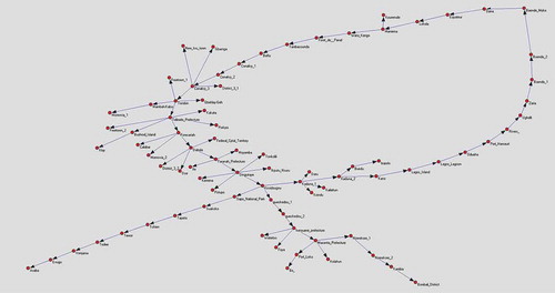
Figure 6 shows the main cause of the Ebola outbreak is at Kissidougou and is located in the forested area in the south eastern of Guinea this was confirmed by WHO and MoH of Guinea report as the origin of the outbreak.

We use a new algorithm called Selfie and show the overlap of the results on Google earth (Figure 7). The same data (Table 2) have been used for this analysis.

Figure 7. The overlap of the Selfie result on Google earth. Red dots are the points of the dataset.

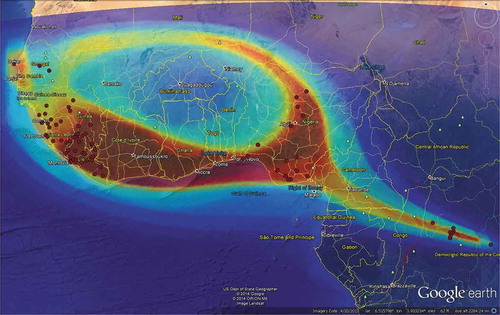
The result from Selfie shows the Ebola outbreak is spreading toward the south of Guinea and mostly Sierra Leone and Liberia and it might spread over other countries if it is not be controlled. The prediction pattern overall formed a ring over a large scale that includes the infected countries.

Ebola Outbreak 2018

The Ebola outbreak in Congo in 2018 was controlled quickly and it did not spread out in the large region. For this case, we have used only TWCα. The Ebola outbreak was reported in 10 places (see Table 3). The largest distance between the outbreak points is the distance between Wangata and Loango which is less than 150 Km. The Ebola outbreak spread out over a triangular region (between Bikoro, Iboko, and Wengata heath zones) with the area of less than 5000 km². Most of the outbreaks were distributed in the regions of Bikoro and Iboko health zones. We have used three set of coordinates corresponding to Bikoro, Iboko, and Wengata heath zones as shown in Table 5 (Ebola virus disease-Democratic Republic of the Congo, Disease outbreak news 2018). The results of the TWCα algorithm predicted the origin of the outbreak at (Longitude: 18.3046, Latitude: −0.6865) in the Equator located in the suburb of Bikoro. This location is at the north west of Bikoro at the distance less than 20 km to Bikoro.

Table 5. The Ebola outbreak dataset that has been used for the TWCα algorithm to predict the origin of the outbreak in Congo (May 2018).

Location	Latitude	Longitude
Wangata	0.0332	18.2348
Bikoro	−0.7317	18.1399
Iboko-bolombi	−1.1847	18.7486

Conclusion

In this paper Topological Weighted Centroid (TWC), Dynamic Naive Bayesian (DNB) Algorithm, and Selfie ANN were used.

In this paper three different Topological Weighted centroid, TWC, algorithms, TWCα, TWCβ, and TWCγ were applied to the Ebola outbreak data that were extracted from HealthMap. Our results show the main origin of the outbreak is in the forested area in south eastern Guinea and that has been confirmed by WHO and MoH of Guinea as being the source of Ebola. The TWCβ algorithm captures two secondary regions in addition to the main region of the outbreak but TWCγ algorithm in addition to the main region captures only one secondary region. This indicates that the secondary region captured by both the TWCβ and TWCγ algorithms is more important than the region that was captured only by TWCβ. The secondary regions can be considered as the new cause of the outbreak.

The DNB algorithm has elicited the cause-effect logic of the virus scattering and these findings also seem to be reasonable. The DNB algorithm predicted the main cause of the Ebola outbreak is at Kissidougou and is located in the forested area in the south eastern of Guinea.

The Selfie ANN was used to predict the future diffusion of the virus from September 2014. The updated data from WHO has confirmed this predictive scenario (see Table 6). Only Nigeria was overestimated, but the Nigerian authorities worked a lot to stop the virus diffusion after the first contamination (Stephen and Sabeti 2014). Further, Selfie ANN suggests a circular area which is specific to an Ebola diffusion in West Africa. But according to the Selfie prediction, the center of this area should be completely safe (around Burkina Faso), and the future data coming from WHO has confirmed this estimation. At this point a question arises: why? Analysis of the flora and fauna of this area would be useful in order to know if some natural inhibitor of the virus was active in that area.

Table 6. New cases from September 2014 (Source: http://healthmap.org/ebola/#).

New Cases from	1 September 2014	To 6 October 2014	Increment
Guinea	648	1199	85.03%
Sierra Leone	1026	2437	137.52%
Liberia	1378	3834	178.23%
Nigeria	17	20	17.65%
DR Congo	24	70	191.67%

We have also used the TWCα algorithm to predict the origin of the Ebola outbreak in DR Congo in 2018. The algorithm predicts the origin is in the suburb of Bikoro that is matched with WHO’s reports.

Acknowledgments

We would like to thank “Quantic Nivi Group” for their great service for superimposing our results on the regional maps.

Disclosure statement

The authors declare that there is no conflict of interest regarding the publication of this paper.

References

- Buscema, M. 2015. Why Mathematical Computer Simulations Are the New Laboratory for Scientists. Substance Use & Misuse 50 (8–9):1068–78. doi:10.3109/10826084.2015.1012934.
- Buscema, M., M. Breda, and G. Catzola. 2009. The topological weighted centroid, and the semantic of the physical space – Theory. In Artificial Adaptive Systems in Medicine, ed. M. Buscema and E. Grossi, 69–78, Bentham Science Publisher: Bentham.
- Buscema, M., E. Grossi, M. Breda, and T. Jefferson. 2009. Outbreaks source: A new mathematical approach to identify their possible location. Physica A 388:4736–62. doi:10.1016/j.physa.2009.07.034.
- Buscema, M., E. Grossi, A. Bronstein, W. Lodwick, M. Asadi-Zeydabadi, R. Benzi, and F. Newman. 2013. A new algorithm for identifying possible epidemic sources with application to the German Escherichia Coli outbreak. ISPRS International Journal Geo- Inf 2:155–200. doi:10.3390/ijgi2010155.
- Buscema, M., G. Massini, and P. Sacco. 2017. The Topological Weighted Centroid (TWC): A topological approach to the time-space structure of epidemic and pseudo-epidemic processes. Physica A 492, 582-627.
- Clubri, A., T. Silver, T. Fradet, K. Retzepi, B. Fry, P. Sabeti, and T. S. Churcher Editor. 2016, Mar. Transforming Clinical Data into Actionable Prognosis Models: Machine-Learning Framework and Field-Deployable App to Predict Outcome of Ebola Patients. PLoS Neglected Tropical Diseases 10(3), 1-17.
- Ebola Virus Disease, Democratic Republic of the Congo, External Situation Report 5, Heath Emergency Information and Risk Assessment, Date of Issue: 25 May 2018, Data as reported by 23 May 2018. http://apps.who.int/iris/bitstream/handle/10665/272662/SITREP-EVD-DRC-20180525-eng.pdf (Accessed: June 2018)
- Ebola virus disease-Democratic Republic of the Congo, Disease outbreak news, 23 May 2018, WHO, http://www.who.int/csr/don/23-may-2018-ebola-drc/en/ (Accessed: June 2018)
- Grossi, E., M. Buscema, and T. Jefferson. 2009. The topological weighted centroid, and the semantic of the physical space – Application. In Artificial Adaptive Systems in Medicine, ed. M. Buscema and E. Grossi, 79–89, Bentham Science Publisher: Bentham.
- Santermans, E., E. Robesyn, T. Ganyani, B. Sudre, C. Faes, C. Quinten, B. W. Van, T. Haber, T. Kovac, R. F. Van, et al. 2016 January 15. Spatiotemporal Evolution of Ebola Virus Disease at Sub-National Level during the 2014 West Africa Epidemic: Model Scrutiny and Data Meagreness.. PloS One 11 (1). doi:10.1371/journal.pone.0147172.
- Stephen, S., and P. Sabeti, To stop Ebola, US must be able to diagnose it quickly, Boston Globe, OCTOBER 12, 2014.
- Sylvain, B., et al. 2014. Emergence of Zaire Ebola virus disease in Guinea. The New England Journal of Medicine 371 (15):1418–25. doi:10.1056/NEJMoa1404505.
- Update on the Ebola outbreak in Democratic Republic of Congo, Medicines Sans Frontiers, Doctor without Borders, May 29, 2018, https://www.doctorswithoutborders.org/article/update-ebola-outbreak-democratic-republic-congo?source=ADD180U0U00&utm_source=AdWords&utm_medium=ppc&utm_campaign=GooglePaid&utm_content=nonbrand&gclid=EAIaIQobChMI8r_-uYnH2wIVUoN-Ch1xkQ6aEAAYASAAEgIB0_D_BwE (Accessed: June 2018)
- Wayne, T. A., L. W. Enanoria, F. Liu, D. Gao, S. Ackley, J. Scott, M. Deiner, E. Mwebaze, W. Ip, T. M. Lietman, et al. 2015. Editor, Evaluating Subcriticality during the Ebola Epidemic in West Africa. PloS One 10 (10), 1-10.
- WHO Ebola Response Team. 2014. Ebola Virus Disease in West Africa-The First 9 Months of the Epidemic and Projections. The New England Journal of Medicine 371 (16). doi:10.1056/NEJMoa1411100.
- http://www.who.int/en/, (Accessed: September 2014)
- http://healthmap.org/ebola, (Accessed: September 2014)
- http://data.worldbank.org, (Accessed: September 2014)
- https://www.google.com/maps, (Accessed March 2015)
- http://open.mapquest.com/, (Accessed: March 2015)
- http://www.nhc.noaa.gov/gccalc.shtml, (Accessed: September 2014)