Optimal Input Variables Disposition of Artificial Neural Networks Models for Enhancing Time Series Forecasting Accuracy

ABSTRACT

Artificial Neural Networks (ANNs) models play an increasingly significant role in accurate time series prediction tools. However, an accurate time series forecasting using ANN requires an optimal model. Hence, great forecasting methods have been developed from optimized ANN models. Most of them focus more on input variables selection and preprocessing, topologies selection, optimum configuration and its associated parameters regardless of their input variables disposition. This paper provides an investigation of the effects of input variables disposition on ANNs models on training and forecasting performances. After investigation, a new ANNs optimization approach is proposed, consisting of finding optimal input variables disposition from the possible combinations. Therefore, a modified Back-Propagation neural networks training algorithm is presented in this paper. This proposed approach is applied to optimize the feed-forward and recurrent neural networks architectures; both built using traditional techniques, and pursuing to forecast the wind speed. Furthermore, the proposed approach is tested in a collaborative optimization method with single-objective optimization technique. Thus, Genetic Algorithm Back-Propagation neural networks aim to improve the forecasting accuracy relative to traditional methods was proposed. The experiment results demonstrate the requirement to take into consideration the input variables disposition to build a more optimal ANN model. They reveal that each proposed model is superior to its old considered model in terms of forecasting accuracy and thus show that the proposed optimization approach can be useful for time series forecasting accuracy improvement.

Introduction

In many domains of engineering (Feng, Zhou, and Dong 2019; Shahrul et al. 2018) climatology (Sher and Messori 2019), demography (Folorunso et al. 2010), Chemistry (Damir, Ricardo, and Aznarte 2019), finance (Soui et al. 2019) (Wang, Huang, and Wang 2012), mechanics (Alevizakou, Siolas, and Pantazis 2018), energy (Kuo and Huang 2018a), and many more, there is the common necessity of accurate forecasting the future evolution of an activity through past measurements of it. Hence, several ideas of forecasts in order to improve the Time Series Forecasting (TSF) accuracy have been explored widely (Mendes Dantas and Cyrino Oliveira 2018). Artificial Intelligent (AI), especially the Artificial Neural Networks (ANNs) are widely used and demonstrated to have powerful for stochastic systems modeling and TSF, and easy implementation and combination with others in a different way compared with other existing forecasting tools (Kuo and Huang 2018a, 2018b). An accurate TSF requires an optimal ANN model based. These optimal models are commonly achieved by modifying the ANN learning paradigm and parameters such as nodes, weights, activation functions, and structures (Crone and Kourentzes 2009).

Nowadays, several efforts have been made in the development and applications of ANNs, mainly oriented toward the improvement of their optimization-based TSF. These existing optimization approaches are based on optimal parameters and minimum model structure of neural networks (Reza Loghmanian et al. 2012; Zongyan and Best 2015). The time-series input variables represent an external parameter of an ANN architecture. They are commonly collected at a different order of magnitude and relations with the target variable. Great publications have shown the adequate input variables as one of the most important parameters for an optimal ANN and accurate TSF (Crone and Kourentzes 2009). They influence the forecasting accuracy through the number of nodes, the length and the relation between them, and each of them and target (Wei, Yoshiteru, and Shouyang 2004). However, the optimal ANNs architectures have not been analyzed regarding their input variables disposition adequacy in TSF accuracy. Wei et al. (Wei, Yoshiteru, and Shouyang 2004) presented a general approach to determine the input variables of ANNs models for TSF. The proposed approach was based on autocorrelation criterion used to measure the degree of correlation between the neighboring time-series data used as input variables of feed-forward neural networks. Furthermore, Sovann et al. (Sovann, Nallagownden, and Baharudin 2014) proposed a method to determine the input variables for the ANN model; Autocorrelation, partial autocorrelation, and cross-correlation are used to measure the correlated input variables with target variable to increase the accuracy of Multilayer Perceptron neural networks architecture based on electrical load demand prediction. Yaïci et al. (Yaïci et al. 2017) studied the effect of reduced inputs of ANNs on the predictive performance of the solar energy system. The results of study show that the degree of feed forward predicting model accuracy would gradually decrease with reduced input variables number. Moreover, there is a great work proposed in the literature which used various types of optimization techniques and algorithm to determine the optimal ANN models and combined models for accurate TSF improvement applied in many domains. Among the most prominent techniques is the Single-Objective optimization technique such as Evolutionary Algorithm, and Genetic Algorithm (Hassan and Hamada 2018; Loghmanian, Ahmad, and Jamaluddin 2009). Piazza et al. (Di Piazza, Di Piazza, and Vitale 2016) combined Genetic Algorithm (GA) and Optimal Brain Surgeon (OBS) strategy to determine the optimal nonlinear autoregression with exogenous input neural networks architecture to forecast wind speed and solar radiation. The optimization techniques of developed neural networks were based on optimal hidden neurons, biases, and weights determination. Therefore, it can be noticed that the optimization techniques of ANNs architectures based on accurate TSF presented in the literature have been limited on optimal input nodes, hidden nodes and weight, learning paradigm and so on, regardless of the input variables disposition. Unlike the traditional optimal input variables of an ANN determination method, the purpose of this study is to quantify the optimal disposition of input variables for an optimal ANN model based on accurate TSF.

The environmental problems, such as climate change, pollution, and global warming from the human activities reduce the development of sources of renewable energy in replacing the polluting sources as fossil fuels energy (Kuo and Huang 2018a, 2018b; Yaïci et al. 2017). Furthermore, the electricity demand and water pumping are steadily increasing as a consequence of world population growth throughout the world (Kuo and Huang 2018a). The sources of green energy such as wind energy potential are free and available in any part of the world, which give a great alternative in terms of electricity production and water pumping. As many sources of renewable energy, wind energy is an intermittent source of energy due to the random fluctuation of wind, since the generated power from a wind energy conversion system has an intimate relationship with the curve of wind speed. Wind speed could be easily influenced by obstacle and terrain (Jursa and Rohrig 2008; Kadhem et al. 2017; Sanchez 2006). Also, it varies from site to site and from height to height. Therefore, accurate wind speed forecasting is required for the wind energy integration (Kadhem et al. 2017; Shen, Wang, and Chen 2018). This will help the electrical production units decentralization and producers take decisions in order of energy production assessment, planning, and management. The recent researches have shown that the ANN model is good at nonlinear modeling and TSF of the stochastic nature of wind speed (Shen, Wang, and Chen 2018).

This work aims at investigating the effect of Input Variables Disposition (IVD) of two ANNs architectures in order to determine their optimal models pursuing to the horizontal TSF. Feed-forward and nonlinear autoregression with exogenous input neural networks were developed using the optimization method given in the literature: the Kolmogorov’s theorem is used to determine the number of hidden nodes and the autocorrelation method was used to select a large number of input nodes. The arrangement formula was applied to determine the number of models of each neural networks architecture through their IVD. A modified Back-Propagation neural networks (BPNN) training algorithm is proposed in this paper, by taking into consideration the IVD. This proposed optimization approach is able to be used in every method using ANN as an old Back-Propagation approach. Thus, it was tested in combining Genetic Algorithms with neural networks to the weighted update. The optimal IVD was provided through the better forecasting performance of the optimized ANN model. The paper is organized as follows: Section 2 provides a description of both ANNs architectures designing, optimization, and models construction based on TSF. The framework of effects of the IVD on neural networks performances investigation is given in Section 3. Section 4 presents the details of the proposed neural networks optimization approach. The results of the study of the effects of the IVD investigation and the forecasting results of the proposed ANNs models and comparison models are presented and discussed in Section 5. In Section 6, relevant conclusions are drawn based on the results achieved from the study case.

Related Forecasting Methodology

Neural Networks and TSF

The TSF is a process which consists of estimating the future value of an activity over time (Alevizakou, Siolas, and Pantazis 2018). To handle TSF, broad methods have been developed. These methods can be broadly classified into physical, statistical, and hybrid (Jursa and Rohrig 2008; Kadhem et al. 2017). Physical method aims by physical consideration, in other words, this method uses the mathematical population modeling, while the statistical method process works by finding the relationship between the measured populations. A hybrid method combines two different methods in order to obtain a globally optimal forecasting performance (Zhang et al. 2017). In recent years, the statistical methods based on ANNs are catching researcher’s attention. Nowadays, ANNs are the most TSF tools used in different fields due to their higher forecasting performance, capacity, flexibility, and robustness (Gogas, Papadimitriou, and Agrapetidou 2018; Kuo and Huang 2018b).

ANN is an information processing structure inspired by human nervous systems (Kuo and Huang 2018b). It consists of networks of many simple units, neurons, operating in parallel which the commonly used have three layers, one input layer, one or more hidden layers, and one output layer (Kuo and Huang 2018a; Yaïci et al. 2017). An ANN learns from given sample examples, by constructing the relationship between input and target variables (Cervone et al. 2017). This process helps to update the synaptic weights of the connections between nodes. As the learning processes, the ANNs can differ through their structures, also called architectures (State, Uyo, and Offiong 2016). The widely ANNs architectures used in TSF can be classified into static and dynamic neural networks.

Static Neural Networks

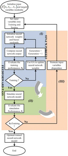
The Feedforward Neural Networks (FFNN) also called static neural networks allow information to travel only from input to output. There is no feedback and memory. FFNN tend to be a straightforward network that associates inputs with outputs. The Multilayer Perceptron’s with FFNN architecture is more used in many different types of applications (Kuo and Huang 2018a). Its greatest strength is in non-linear solutions to ill-defined problems (Crone and Kourentzes 2009). Figure 1 illustrates the architecture of an FFNN with one hidden layer, yellow, intended to the TSF.

Figure 1. FFNN architecture intended to the TSF.

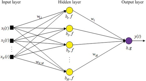
From Figure 1, the input layer, black, is made of N nodes, $[x_1(t),x_2(t),\dots ,x_N(t)]$, constituting the number of past data used as input variables of ANN, hidden layer has M nodes, yellow, and output layer have only one node, purple constructing the forecasting variable. t represents the sample time steps. The output of the hidden layer is calculated as follows:

(1) $\begin{array}{c}{h}_i(t)=f\left(\sum _k^N{w}_{k,i}.x_k(t)-b_i\right),{\hspace{0.17em}}_k=1,2,\dots ,N,{\hspace{0.17em}}_i=1,2,\dots ,M\end{array}$(1)

where $h_i(t)$ is the output of the node of the hidden layer at a time step $t$, $w_{k,i}$ is the connection parameter, synaptic weight, between the k node of the input layer and the i node of the hidden layer, $b_i$ is bias of the i node of the hidden layer and f is the activation function used in each node of the hidden layer. The evaluation of the forecasting variable at the output layer is expressed as follows:

(2) $y(t)=g\left(\sum _i^M{w}_{i,y}.h_i(t)-b_y\right),{\hspace{0.17em}}_i=1,2,\dots ,M$(2)

where $y(t)$ is the forecasting variable at a time step $t$ at the output layer, $w_{i,y}$ is the synaptic weight which connects the $i$ node of the hidden layer and the alone node of the output layer, $b_y$ and g are the bias and activation function, respectively, of the output node.

Then, the forecasting variable from the developed FFNN is finally designed as

(3) $y(t)=g\left[\sum _i^M{w}_{i,y}.f\left(\sum _k^N{w}_{k,i}.x_k(t)-b_i\right)-b_y\right]$(3)

where the optimal N and M are set in subsection 2.2, in response to the FFNN structure optimization.

Dynamic Neural Networks

Contrary to the previous FFNN structure, the second ANN architecture, Feedback neural networks also called Recurrent Neural Networks (RNN), or dynamic neural networks have signals traveling in both directions by introducing loops in the network (State, Uyo, and Offiong 2016). Consequently, an internal state of the RNN is created displaying a dynamic temporal behavior. The dynamic driven RNN called Nonlinear Autoregressive with exogenous inputs Neural Networks (NARX NN) is well suited to learn nonlinear dynamic systems or time-series relationships (Di Piazza, Di Piazza, and Vitale 2016). A NARX NN is a RNN with global feedback coming only from the output layer rather than by the hidden states. It consists of an FFNN which takes as inputs a window of past independent (exogenous inputs) and past outputs (endogenous inputs), and determines the current output (Zongyan and Best 2015). So, only the output of NARX NN is fed back to the FFNN. NARX NN architecture exists in open-loop and closed-loop (Di Piazza, Di Piazza, and Vitale 2016). Figure 2 presents the NARX NN architectures aimed to the TSF.

Figure 2. NARX NN architecture based on TSF: open-loop (a) and closed-loop (b).

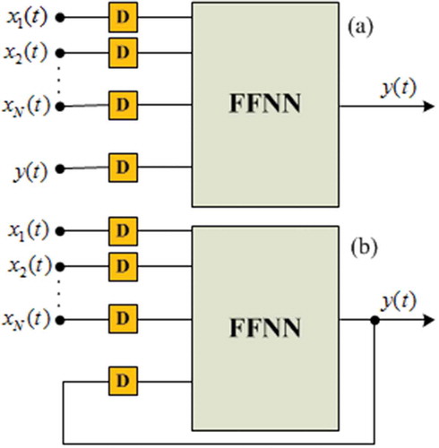
NARX NN is designed as a class of discrete-time nonlinear systems and can be expressed mathematically as follows (Di Piazza, Di Piazza, and Vitale 2016):

(4) $\begin{array}{rl}& y(t)=\mathrm{\Gamma }\left[y(t);x_1(t);x_2(t);\dots x_N(t)\right]\\ & =\mathrm{\Gamma }\left[y(t-1),y(t-2),\dots ,y(t-u_y);\right.x_1(t),x_1(t-1)\dots {,}_1(t-u_{x_1});x_2(t),x_2(t-1)\dots ,x_2(t-u_{x_2});\dots ;\\ & \left.x_N(t),x_N(t-1),\dots ,x_N(t-u_{x_N})\right]\end{array}$(4)

where $y(t)$ is the current output, endogenous input, and $x_1(t)$, $x_2(t)$, …, $x_N(t)$ are the exogenous inputs at a time step t, D is the time delay line, $\mathrm{\Gamma }$ is an unknown mapping nonlinear function, and $u_y\ge 1$, $u_{x_1}=u_{x_2}=\dots =u_{x_N}$ are the inputs and output memory orders.

Neural Networks Models Optimization

Whatever ANN architecture, choosing an appropriate parameter is crucial to build an efficient forecasting model. In order to estimate the optimal FFNN and NARX NN architectures developed in the previous subsection 2.1 based on IVD investigation tested on more wind speed forecasting accuracy in this paper, the optimization methods presented in the literature by various authors were applied in each parameter of the networks. The method of autocorrelation was used to select the optimal input variables of neural networks. Therefore, the Spearman’s rank correlation method was applied to determine the relation between past variables (see Table 1) (Upadhyay, Choudhary, and Tripathi 2011). After correlation determination, a maximum of four weather variables were chosen to be used as input variables of both neural networks, Since Yaïci et al. (Yaïci et al. 2017) provide that the forecasting performance of ANNs increases as the number of input nodes increases. Therefore, the past-selected input variables are air temperature (Ta), atmospheric pressure (Pa), relative humidity (RH), and the past wind speed (Ws) is the target of both ANNs. Also, the time step variation (T) is used as the input variable of both ANNs architectures. Wei et al. (Wei, Yoshiteru, and Shouyang 2004) shown that the forecasting accuracy decreases as the training and forecasting data size increases. This criterion of ANNs optimization is not considered in this work. Therefore, a large size of the past data was recorded for 3 months with 10 minute intervals, 10573 datasets in the west region of Cameroon. The used variables for the present work and the results of the coefficient of correlation between them, obtained numerically are presented in Table 1.

Table 1. Relations between the actual variables.

	Ws	Ta	Pa	RH	T
Ws	1	0.3119	0.0432	−0.4859	−0.2631
Ta		1	0.2198	−0.5864	0.0175
Pa			1	−0.0761	0.0702
RH				1	−0.0457
T					1

Table 1 gives the values of the correlation coefficients between the output variable and each input variable as well as between the input variables themselves. Thus, we can see from Table 1 that there are smaller relations between the input variables and the target variable.

According to the Kolmogorov’s theorem applied to determine the optimal number of hidden nodes of both ANNs architectures, for the three-layer neural networks as developed in this work, the number of hidden neurons is recommended as $M=2N+1$ (Peng, Liu, and Yang 2013). Therefore, each developed ANN architecture had nine hidden nodes, $M=9$.

Neural Networks Models Building

We have chosen four variables to use as input variables of optimized static and dynamic neural networks architectures, aimed to better the accurate TSF. To study the influence of the IVD of each developed ANN on the training and TSF performances, we had used the mathematical formula of arrangement to determine the number of possible disposition of the chosen input variables. Thus, the way input variables were disposed defines the neural networks model. It can be expressed by Equation (5)(5) $Mo=N!$(5) :

(5) $Mo=N!$(5)

where $Mo$ is the possible number of ANNs models. Therefore, using the four chosen input variables, each of the developed ANNs structures had 24 models, $Mo=25$ which were trained and tested to forecast one day-ahead of wind speed.

Forecasting Accuracy Evaluation

In order to investigate the performances of forecasting models, three errors criterion were taken into consideration. The Root Mean Square Error (RMSE), expressed as follows:

(6) $RMSE=\sqrt{\frac{1}{T}\sum _{t=1}^T{\left(y{(t)}_m-y{(t)}_p\right)}^2}$(6)

was used to measure the efficiency of the developed prediction tools in projecting future individual values. A smaller and more positive RMSE indicates a considerable convergence of the forecasted values and the real values. The Mean Absolute Error (MAE) is used to measure the long-term model forecasting, is defined as:

(7) $MAE=\frac{1}{T}\sum _{t=1}^T\left|\left(y{(t)}_m-y{(t)}_p\right)\right|$(7)

The Mean Absolute Percentage Error (MAPE) was used to establish the forecasting accuracy. It indicates in percentage the accuracy in fitting time series values in statistics in a particular trend. It is defined by the following equation:

(8) $MAPE=\frac{1}{T}\sum _{t=1}^T\left|\frac{y{(t)}_m-y{(t)}_p}{y{(t)}_m}\right|\times 100$(8)

where $y(t{)}_m$ and $y(t{)}_p$ are the real and forecasted values, respectively, at the time step t, and T is the number of time step.

Effects of the IVD on Neural Networks Performances Investigation

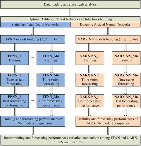
Figure 3 indicates the steps followed to evaluate the influence of the IVD on both neural networks structures performances. All the developed ANNs models used the same common parameters. The tangent hyperbolic sigmoid and linear functions are used as activation functions of each hidden node and output node, respectively. The Lavenberg marquardt back-propagation algorithm is used to train the neural networks models following the error detection method. The NARX NN models were trained using its open-loop architecture and the multi-step forecasting was carried out with its closed-loop architecture. Several delays have been tried and the better results from NARX NN models had been achieved with four delays per variable, D = 4. Before the training process of neural networks models, the data sets are brought within the same order of magnitude. Thus, every data have been normalized between 0 and 1.

Figure 3. Flowchart of effects of input variables disposition of neural networks investigation.

Proposed Neural Networks Optimization Approach

Table

Algorithm: Proposed neural networks based forecasting approach

Objective:

Minimize the forecasting errors through the optimal input

variables of neural network disposition

Inputs:

X–Input variable

Xtr – Training input variable

Xs – Validation input variable

Xt – Testing input variable

Outputs:

Y – Forecasting variable

Ytr – Training target variable

Ys – Validation target variable

Parameters:

N – Number of input variables

Esmin – Minimum validation neural network performances

Tmax – Maximum retraining iteration

1. $X=[x_1,x_2,\dots ,x_N]$

2. Set target into Ytr and Ys

3. for $i=1$ to N! do

4. $X_i=permute(X_i)$

5. Set $X_i$ into Xtr, Xs and Xt

6. Set neural network architecture and parameters

7. for j = 1 to Tmax do

8. Randomly initialize neural network weights and biases

9. Train neural network model

10. $S_i^j=Simulate(neural{\hspace{0.17em}}_{n}etwork)$

11. $E{s}_i^j=errors(S_i^j,Ys)$

12. if $E{s}_i^j<Esmin$ then

13. break

14. end if

15. end for

16. for k = 1 to length(Xt) do

17. $O_i^k=predict(neural{\hspace{0.17em}}_{n}etwork,Xt{r}_i^k)$

18. end for

19. $E{f}_i=errors(O_i^k,Yf)$

20. if $E{f}_i<E{f}_{i-1}$ then

21. $Ef=E{f}_i$

22. $Y=O_i^k$

23. else

24. $Ef=E{f}_{i-1}$

25. $Y=O_i^{k-1}$

26. end if

27. end for

28. return Ef

29. return Y

The goal of the proposed approach is to find the optimal IVD for a more optimal neural network solution. The neural networks are trained with modified Back-Propagation (BP) algorithm by introducing the IVD consideration. The traditional BP algorithm is used to update the neural networks weights with a random initial IVD. The IVD is permuted and the neural network is retrained to obtain an optimal solution. Figure 4 draws the flowchart of the proposed modified BPNN training algorithm. As shown in this Figure 4, the proposed modified BPNN have three main stages: Stage (I) is the traditional BPNN training algorithm constituted by a feed-forward pass, which consists to take an input variable to express the corresponding output through the synaptic weights, and a feedback pass which aims to update the neural network weights. At the end of this training process, the neural network is validated in the stage (II) by simulating its ability to generalize the desired output. This stage (II) allows to avoid the overlearning or overfitting, and to find the optimal model. Stage (III) is the added feedback pass, which allows to retrain the neural network (back to stage (I)) for each IVD until the better solution is obtained.

Figure 4. Flowchart of proposed BPNN with optimal IVD searching.

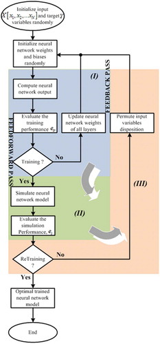
The modified BPNN was proposed for improving TSF accuracy for 1 day ahead wind speed. The detail of the modified BPNN based on TSF is presented in Algorithm. As in the training process, the retraining process is controlled through the validation performances, $e_s$, and the number of retraining iteration, $T_{max}>Mo$.

The proposed modified BPNN are able to be used in combining model as the traditional BPNN. Then, this proposed optimization approach was evaluated in combining Genetic Algorithm (GA) and neural networks. Here, the GA was used to find the optimal weights of neural networks in the feedback pass of the stage (I). This for different possible IVD until an optimal solution is obtained. Figure 5 indicates the whole process of BPNN optimization by GA and IVD consideration.

Figure 5. Proposed BPNN optimization by GA and IVD consideration.

Experimental Results and Discussion

IVD and Neural Networks Performances

After both neural networks architectures setting and models are constructed in order to investigate the influence of IVD on forecasting accuracy, the sought of best training and forecasting performance of each model is required. Thus, there are 10 simulations each of them with 10430 datasets. Three months were used in the training process and tested to forecast the short-term wind speed. The better performances of these simulations are considered for each of the developed neural networks models. Table 2 lists the different IVD, training, TrPerform, and forecasting performances of each of the models for FFNN and NARX NN architecture, respectively.

Table 2. Statistical performances of ANNs models.

	Models			FFNN			NARX NN
No	disposition	TrPerform	RMSE	MAE	MAPE(%)	TrPerform	RMSE	MAE	MAPE(%)
1	Ta-Pa-RH-T	0.0791	1.9017	1.6215	20.095	0.0294	1.113	0.883	16.4035
2	Ta-Pa-T-RH	0.0803	1.3936	1.0975	20.185	0.0291	1.0973	0.859	16.1747
3	Ta-T-Pa-RH	0.0785	1.4431	1.1681	20.934	0.0297	1.2409	0.963	16.7212
4	Ta-T-RH-Pa	0.0791	1.395	1.1116	20.64	0.0294	1.2684	0.971	16.7102
5	Ta-RH-T-Pa	0.0789	1.4144	1.0663	18.651	0.0293	1.4272	1.074	18.6297
6	Ta-RH-Pa-T	0.0792	1.4026	1.0857	19.498	0.029	1.1854	0.917	17.3096
7	Pa-Ta-RH-T	0.0782	1.4697	1.2028	20.893	0.0293	1.1796	0.949	18.1993
8	Pa-Ta-T-RH	0.0788	1.4917	1.1592	19.115	0.0292	1.23	0.961	16.764
9	Pa-T-RH-Ta	0.0772	1.3431	1.0619	19.349	0.0293	1.1973	0.946	17.4748
10	Pa-RH-T-Ta	0.0787	1.326	1.0773	19.767	0.0295	1.1973	0.946	17.4748
11	Pa-RH-Ta-T	0.0794	1.2934	1.0183	19.626	0.0291	1.1305	0.906	16.7442
12	Pa-T-Ta-RH	0.0796	1.5071	1.0987	19.259	0.0295	1.0449	0.843	15.205
13	RH-Pa-T-Ta	0.0798	1.3811	1.0525	18.485	0.0294	1.0685	0.852	16.01
14	RH-Pa-Ta-T	0.0781	1.3726	1.0856	19.422	0.0292	1.1088	0.885	15.9322
15	RH-T-Pa-Ta	0.0819	1.3763	1.0549	19.138	0.0289	1.1074	0.878	15.1771
16	RH-Ta-Pa-T	0.0796	1.4609	1.1652	20.494	0.029	1.199	0.938	16.4563
17	RH-T-Ta-Pa	0.0819	1.3763	1.0549	19.138	0.0293	1.0387	0.824	14.1664
18	RH-Ta-T-Pa	0.0787	1.4118	1.1257	20.119	0.0289	1.3709	1.039	17.4982
19	T-RH-Pa-Ta	0.0786	1.3433	1.0892	20.382	0.0293	1.0106	0.823	15.4901
20	T-Pa-RH-Ta	0.0797	1.3584	1.0463	18.577	0.0292	1.1174	0.904	16.7915
21	T-RH-Ta-Pa	0.0781	1.3128	1.0657	19.772	0.0293	1.2105	0.977	16.8154
22	T-Ta-RH-Pa	0.0799	1.4297	1.1122	19.148	0.0293	1.0846	0.88	16.525
23	T-Ta-Pa-RH	0.08	1.3492	1.0258	18.475	0.0292	1.0378	0.823	14.9924
24	T-Pa-Ta-RH	0.0781	1.3489	1.0777	19.255	0.0292	1.0332	0.829	15.1903

According to the results presented in Table 2, all the models of both ANNs structures have different performances. In other words, the training and forecasting performances are varying according to the ANNs models. The difference between the minimum and maximum value of a performance criterion is evaluated in percentage using Equation (9)(9) $P_{Error}=\left(\frac{Erro{r}_2-Erro{r}_1}{Erro{r}_2}\right)\times 100$(9) . For the FFNN architecture, the training performance, TrPerform, varies from 0.0772 to 0.0819, 5.73%; the forecasting errors RMSE, MAE, and MAPE vary from 1.2934 to 1.9017, 31.98%, from 1.0183 to 1.6215, 37.20% and from 18.4749 to 20.9336, 11.74%, respectively. For the NARX NN architecture, the training performance, TrPerform, varies from 0.0289 to 0.0297, 2.69%; the forecasting errors RMSE, MAE, and MAPE vary from 1.0106 to 1.4272, 29.19%, from 0.8227 to 1.074, 23.39%, and from 14.1664 to 18.6297, 23.95%, respectively. These significant differences between each better and worse performance criterion indicate the high influence of the input variables disposition upon training and forecasting performances of neural networks models. Meanwhile, among both neural networks, the FFNN structure has the more significant difference between the performance criteria. Therefore, we can conclude that the feedforward neural network is more sensible to IVD than recurrent neural networks. Figure 6 indicates the training and forecasting performances versus models of FFNN structure. Also, Figure 7 shows the training and forecasting performances versus models of NARX structure.

Figure 6. Training, (a), and forecasting, RMSE = (b), MAE = (c), MAPE (%) = (e), performances of FFNN models.

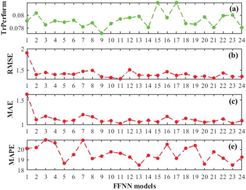
Figure 7. Training, (f), and forecasting, RMSE = (g), MAE = (i), MAPE (%) = (j), performances of NARX NN models.

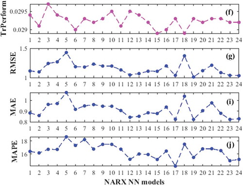
The fluctuations of performances of both developed ANNs architectures according to their models can be clearly observed in Figures 6–7. They clarify the influence of IVD upon static and dynamic neural networks models. Thus, the optimal IVD is required to build the optimal neural networks model based on more accurate TSF.

According to Table 2 and Figures 6–7, the first four most accurate forecasting models of the FFNN and NARX NN structure are the models 5, 20, 13, 23 and 12, 17, 15, 23, respectively. According to Wei, Yoshiteru, and Shouyang 2004 (Feng, Zhou, and Dong 2019), the input variables of an ANN need to have the high strength correlation between each of them and the target variable, but should not be correlated. According to the results presented in Tables 1 and 2, this is confirmed by the models 5 and 13 of the FFNN structure, but not for any NARX NN models. Therefore, based on the above experiments, it can be concluded that: (i) NARX NN structure obtains the most accurate results than FFNN structure. (ii) The way that the input variables disposition influence the neural networks performance is different according to their architectures. (iii) There is a tiny possibility of having an optimal FFNN model by arranging its input variables in such a way as to avoid the strength correlation between two neighboring input variables.

Also, we can see a real similarity in the variations of graphs 6(b), 6(c), and 6(e). This similarity is more considerable between graphs 7(g), 7(i), and 7(j). These similarities confirm the stability of the match of IVD with forecasting performances of the neural networks models. But these similarities are smaller between the training graph, 6(a), and the forecasting graphs, 6(b), 6(c), and 6(e). Event between 7(f) and 6(g), 6(i), and 6(j). Thus, these lack of concordance between the training performances and those of forecasting reflect the fact that some IVD are subject to overlearning or overfitting, e.g., models 12 and 18 of NARX NN and model 7 of FFNN. To further illustrate this, Table 3 gives the coefficients of correlation between the performances criteria from the two ANNs architectures.

Table 3. Relations between the performance criteria.

ANN		TrPrform	RMSE	MAE	MAPE	ANN
	TrPrform		−0.0651	−0.0317	0.0276	NARX NN
	RMSE	0.0073		0.9860	0.798
	MAE	0.1369	0.9526		0.8450
FFNN	MAPE	−0.3116	0.222	0.3989

The most remarkable observation in these results from Table 3 is the smaller relations between training and forecasting errors criteria. They also argue that there are strong relations between the forecasting errors from NARX NN models than FFNN. Therefore, we can conclude that the forecasting performance of NARX NN is less sensitive than that of FFNN to overlearning or overfitting that some IVD may cause.

Proposed Forecasting Models Evaluation

This section describes the experiments conducted to examine the performance of the proposed neural networks optimization approach, which was based on IVD pursing to enhance TSF accuracy. The proposed forecasting models in this work were then based on this proposed optimization approach. Therefore, the FFNN, NARX NN, and GABPNN models were proposed. The proposed GAPBNN model is based on the model proposed by Rahman et al. (Mijanur Rahman and Akter Setu 2015). To perform the evaluation of the forecasting ability of these proposed models, an another commonly used neural network forecasting model is used as the benchmark model, i.e., Adaptive Neuro-Fuzzy Inference System (ANFIS)(Cervone et al. 2017). Table 4 shows the experimental parameters of developed forecasting models.

To ensure that the final results are reliable and independent of the initial random weight and bias values of the proposed models, each developed model is repeated 10 times. It had been shown in the previous subsection 5.1 that the IVD influence the training and forecasting performance of neural networks. Therefore, we will take the better forecasting models of FFNN and NARX NN from Table 2 as comparison models of the proposed models, i.e., models 20 and 17, respectively. Equation (9)(9) $P_{Error}=\left(\frac{Erro{r}_2-Erro{r}_1}{Erro{r}_2}\right)\times 100$(9) is used to describe the improvement percentage of the proposed models over the comparison models, it is defined as,

(9) $P_{Error}=\left(\frac{Erro{r}_2-Erro{r}_1}{Erro{r}_2}\right)\times 100$(9)

where Error represents each statistical error defined in Equations (6)–(6) $RMSE=\sqrt{\frac{1}{T}\sum _{t=1}^T{\left(y{(t)}_m-y{(t)}_p\right)}^2}$(6) (8(8) $MAPE=\frac{1}{T}\sum _{t=1}^T\left|\frac{y{(t)}_m-y{(t)}_p}{y{(t)}_m}\right|\times 100$(8) ), subscript 1 indicates a proposed model, and the subscript 2 gives a comparison model. When a $P_{Error}$> 0, the proposed forecasting model is better than the comparison model and vice versa. The closer $P_{Error}$ to 0, the smaller the difference between the two evaluation errors. The forecasting performance results of the proposed models and the comparing models of the study case are presented in Table 5.

Table 4. Forecasting models parameter settings.

Models	Parameters	Values
FFNN	maximum iterations	1000
	validation check	500
	maximum retraining iterations	100
	layers	02
NARX NN	maximum iterations	1000
	validation check	500
	maximum retraining iterations	100
	delay	04
	layers	02
ANFIS	number of membership functions	02
	number of membership	Gaussian
	maximum epochs	1000
	layers	02
GA	maximum generations	2000
	fitness limit	${10}^{-5}$
	convergence tolerance	${10}^{-10}$

Table 5. Forecasting performance evaluation of different models.

Models	RMSE	MAE	MAPE(%)
ANFIS	1.3456	1.0814	19.6528
GABPNN	1.2115	1.0231	18.3718
Proposed NARX NN	1.0289	0.8037	14.2817
Proposed FFNN	1.1617	0.9009	15.8855
Proposed GABPNN	1.2753	0.9901	16.5621

According to Table 5 the GABPNN model forecasts well than the ANFIS model. Meanwhile, the proposed NARX NN model performs well the TSF than the proposed FFNN and GABPNN models, while ANFIS is the worse one. In Figure 8 the results of forecasting performances from the different proposed and comparing models are drawn. Table 6 gives the performances of forecasting improvement of the proposed models over the comparison models.

Table 6. Improvement percentages of the proposed models.

	Models	FFNN	NARX NN	GABPNN	ANFIS
RMSE	Proposed NARX NN	21.62%	0.940%	15.07%	23.53%
	Proposed FFNN	11.50%	−11.84%	4.110%	13.66%
	Proposed GABPNN	2.85%	−16.91%	−5.260%	5.220%
MAE	Proposed NARX NN	24.58%	2.220%	21.44%	25.67%
	Proposed FFNN	15.46%	−9.590%	11.94%	16.69%
	Proposed GABPNN	7.090%	−20.45%	3.220%	8.440%
MAPE	Proposed NARX NN	23.12%	−0.800%	22.26%	27.32%
	Proposed FFNN	14.48%	−12.13%	13.53%	19.16%
	Proposed GABPNN	10.84%	−22.77%	9.850%	15.72%

Figure 8. Bar chart showing the forecasting errors from the proposed and comparison models.

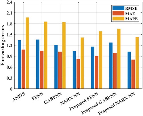
By observing Table 6, we can see that the proposed FFNN model leads to more accurate forecasting performance than the old FFNN model with a considerable difference, by up to 10% for every performance criteria. This shows the effectiveness of proposed FFNN model to perform TSF. Meanwhile, the proposed NARX NN model is being neutralized with the old model, but it obtains the most accurate results among all developed models. It is important to note that this comparison NAX NN model is built with optimal IVD as shown in subsection 5.1. Thus, the proposed NAX NN model can always work as a good forecasting model than the old model which is generally built with random IVD. The results presented in Table 6 show that the combining proposed model, GABPNN is the most accurate model than its old comparison model. The sensitivity of the GABPNN to the arrangement of input variables is clarified in Figure 9, which presents the fluctuation of best fitness values according to the neural networks models.

Figure 9. Best fitness values of GA along with neural networks models.

The research results of the proposed strategy to improve the multi-step TSF performance of ANNs show that the tested models for 24 hours-head wind speed forecasting have the following features: (1) Each proposed model always achieves more accurate value than old one. This shows the effectiveness of the proposed neural networks optimization approach to improve the multi-step head TSF accuracy. (2) Among all the proposed models, FFNN model is the most improved one with the highest improvement percentage values, by up to 10%. Thus, IVD is very important for static neural networks forecasting performances improvement than dynamic neural networks. (3) By using the worse neural networks models of Table 2 as comparison models, we will see that the difference between them and the proposed models will be more considerable.

The presented experiments confirm the competitive forecasting performance of the proposed neural networks models and therefore, show that it will be important to take into consideration the IVD for the optimization of neural networks models. But it was complex to test step-by-step every possible IVD of neural networks aimed to find the optimal one. Thus, the key advantages of the proposed neural networks training and optimization approach are:

- It is possible to test all the possible IVD and the search of the optimal disposition is included in the neural networks training algorithm. Thus, the approach does not require any predisposition of the input variables and relations between them analysis stage.

- The complexity of the approach in terms of computation and speed is much less than step-by-step method used to find the optimal IVD, which facilitates the real-time application of the proposed neural networks optimization approach.

- The forecasting performance is better than that obtained by using other methods to search the optimal IVD such as step-by-step finding and non-correlated input variable methods.

- Possibility to be combined with other techniques to build the hybrid TSF models.

Conclusion

This paper introduces a new framework based on input variables disposition to construct optimal neural networks for more accurate time series forecasting. The investigation carries out on feed-forward and nonlinear autoregression with exogenous neural networks structures to forecast 24 hours ahead wind speed has shown that their training and forecasting performances change according to their input variables disposition. Meanwhile, the input variables disposition do not change the computational time of neural networks models. Thus, the optimal forecasting requires an optimal input variables disposition of ANN based. A new ANN training approach has been proposed; introducing the optimal input variables disposition into Back-Propagation algorithm. This proposed approach has been applied to develop the neural networks forecasting models including combining model using generic algorithm. The numerical results of the study case reveal the effectiveness of the proposed approach and neural networks models to improve accuracy of multi-step head time series forecasting, in which every proposed model improves the performance of its old model. Moreover, this proposed optimization approach could be also used together with the multi-objective algorithms for more time series forecasting models stability and errors minimizing such as bat algorithm, evolutionary algorithm, and firefly algorithm.

Conflicts Of Interest

The authors declare no conflict of interest.

References

- Alevizakou, E., G. Siolas, and G. Pantazis. 2018. Short-term and long-term forecasting for the 3D point position changing by using artificial neural networks. International Journal of Geo-Information 7:1–15.
- Cervone, G., L. Clemente-Harding, S. Alessandrini, and L. D. Monache. 2017. Short-term photovoltaic power forecasting using artificial neural networks and an analog ensemble. Renewable Energy 108:274–86.
- Crone, S. F., and N. Kourentzes, Input-variable specification for neural networks - an analysis of forecasting low and high time series frequency, Proceedings of International Joint Conference on Neural Networks, Atlanta, Georgia, USA, (2009), 619–26.
- Damir, V., N. Ricardo, and J. L. Aznarte. 2019. Forecasting hourly NO2 concentrations by ensembling neural networks and mesoscale models. Neurocomputing 32:9331-9342.
- Di Piazza, A., M. C. Di Piazza, and G. Vitale. 2016. Solar and wind forecasting by NARX neural networks. Renewable Energy Environmental Sustainability 39:1–5.
- Feng, S., H. Zhou, and H. Dong. 2019. Using deep neural network with small dataset to predict material defects. Materials & Design 162:300–10.
- Folorunso, O., A. T. Akinwale, O. E. Asiribo, and A. Adeyemo. 2010. Population prediction using artificial neural network. African Journal of Mathematics and Computer Science 3:155–62.
- Gogas, P., T. Papadimitriou, and A. Agrapetidou. 2018. Forecasting bank failures and stress testing?: A machine learning approach. International Journal of Forecasting 34:40–456.
- Hassan, M., and M. Hamada. 2018. Genetic algorithm approaches for improving prediction accuracy of multi-criteria recommender systems. International Journal of Computational Intelligence Systems 11:146–62.
- Jursa, R., and K. Rohrig. 2008. Short-term wind power forecasting using evolutionary algorithms for the automated specification of artificial intelligence models. International Journal of Forecasting 24:694–709.
- Kadhem, A. A., N. I. Abdul Wahab, I. Aris, J. Jasni, and A. N. Abdalla. 2017. Advanced wind speed prediction model based on a combination of weibull distribution and an artificial neural network. Energies 10:1–17.
- Kuo, P., and C. Huang. 2018a. An electricity price forecasting model by hybrid structured deep neural networks. Sustainability 10:1–17.
- Kuo, P., and C. Huang. 2018b. A high precision artificial neural networks model for short-term energy load forecasting. Energies 11:1–13.
- Loghmanian, S. M. R., R. Ahmad, and H. Jamaluddin, Multi-objective optimization of NARX model for system identification using genetic algorithm, 2009 First International Conference on Computational Intelligence, Communication Systems and Networks, Indore, India (2009), 196–201.
- Mendes Dantas, T., and F. L. Cyrino Oliveira. 2018. Improving time series forecasting: An approach combining bootstrap aggregation. Clusters and Exponential Smoothing, International Journal of Forecasting 34:748–61.
- Mijanur Rahman, M., and T. Akter Setu. 2015. An implementation for combining neural networks and genetic algorithm. International Journal of Computer Science and Technology 6:218–22.
- Mohandes, M., S. Rehman, and S. M. Rahman. 2011. Estimation of wind speed profile using adaptive neuro-fuzzy inference system (ANFIS). Applied Energy 88:1–9.
- Peng, H., F. Liu, and X. Yang. 2013. A hybrid strategy of short term wind power prediction. Renewable Energy 50:590–95.
- Reza Loghmanian, S. M., H. Jamaluddin, R. Ahmad, R. Yusof, and M. Khalid. 2012. Structure optimization of neural network for dynamic system modeling using multi-objective genetic algorithm. Neural Computing and Applications 21:1281–95.
- Sanchez, I. 2006. Short-term prediction of wind energy production. International Journal of Forecasting 22:43–56.
- Shahrul, N. S., R. R. Muhammad, S. Sabrilhakim, and M. K. Mohd Shukry. 2018. Thumb-tip force prediction based on Hill’s muscle model using electromyogram and ultrasound signal. International Journal of Computational Intelligence Systems 11:238–47.
- Shen, Y., X. Wang, and J. Chen. 2018. Wind power forecasting using multi-objective evolutionary algorithms for Wavelet neural network-optimized prediction intervals. Applied Sciences 8:1–13.
- Sher, S., and G. Messori. 2019. Weather and climate forecasting with neural networks: Using general circulation models (GCMs) with different complexity as a study ground. Geoscientific Model Development 12:2797–809.
- Soui, M., S. Smiti, M. W. Mkaouer, and R. Ejbali. 2019. Bankruptcy prediction using stacked auto-encoders. Applied Artificial Intelligence 34:1–21.
- Sovann, N., P. Nallagownden, and Z. Baharudin. 2014. A method to determine the input variable for the neural network model of the electrical system. 5th International Conference on Intelligent and Advanced Systems (ICIAS), Kuala Lumpur, Malaysia (2014), 3-5 .
- State, I., A. Uyo, and A. Offiong. 2016. Neural networks in materials science and engineering: A review of salient issues. European Journal of Engineering and Technology 3:40–54.
- Upadhyay, K. G., A. K. Choudhary, and M. M. Tripathi. 2011. Short-term wind speed forecasting using feed-forward back-propagation neural network. International Journal of Engineering, Science and Technology 3:107–12.
- Wang, B., H. Huang, and X. Wang. 2012. A novel text mining approach to financial time series forecasting. Neurocomputing 83:136–45.
- Wei, H., N. Yoshiteru, and W. Shouyang. 2004. A general approach based on autocorrelation to determine input variables of neural networks for time series forecasting. Journal of Systems Science and Complexity 17:297–305.
- Yaïci, W., M. Longo, E. Entchev, and F. Foiadelli. 2017. Simulation study on the effect of reduced inputs of artificial neural networks on the predictive performance of the solar energy system. Sustainability 9:1–14.
- Zhang, J., Y. Wei, Z. Tan, K. Wang, and W. Tian. 2017. A hybrid method for short-term wind speed forecasting. sustainability 9:1–10.
- Zongyan, L., and M. Best. 2015. Optimization of the input layer structure for feed-forward narx neural networks. International Journal of Electrical and Computer Engineering 9:673–67.