A Novel Method of Curve Fitting Based on Optimized Extreme Learning Machine

ABSTRACT

In this article, we present a new method based on extreme learning machine (ELM) algorithm for solving nonlinear curve fitting problems. Curve fitting is a computational problem in which we seek an underlying target function with a set of data points given. We proposed that the unknown target function is realized by an ELM with introducing an additional linear neuron to correct the localized behavior caused by Gaussian type neurons. The number of hidden layer neurons of ELM is a crucial factor to achieve a good performance. An evolutionary computation algorithm–particle swarm optimization (PSO) technique is applied to determine the optimal number of hidden nodes. Several numerical experiments with benchmark datasets, simulated spectral data and measured data from high energy physics experiments have been conducted to test the proposed method. Accurate fitting has been accomplished for various tough curve fitting tasks. Comparing with the results of other methods, the proposed method outperforms the traditional numerical-based technique. This work clearly demonstrates that the classical numerical analysis problem-curve fitting can be satisfactorily resolved via the approach of artificial intelligence.

Introduction

Curve fitting is the process of finding a parameterized function that best matches a given set of data points. It can be viewed as a function approximation problem in such a way that a certain error measure must be addressed explicitly. Representing the data in a parameterized function or equation has actual significances in data analysis, visualization and computer graphics. Curve fitting can be served as aided tools for many techniques involved modeling and prediction. Particularly, scientists and engineers often notice that the best practice gaining some insight and guide to understand the related scientific phenomenon is to fit a set measured or observed data to an empirical relationship. From the resultant empirical formula, interpolation, extrapolation, differentiation, and finding the maximum or minimum location of the curve can be readily carried out without utilizing a full mathematical treatment based on the underlying theory. In addition, curve fitting is also frequently used to estimate the parameters in a variety of modeling studies. For example, the notch-delay solar model in the climate science has a number of independent parameters, which can be estimated by using a curve fitting method.

To fit a given dataset to a curve, the conventional practice is to select a parameterized function or a set of basis function with consideration of data distribution. Then a numerical method for the least-squares approximation with regard to minimizing the sum of squared residuals of data points is applied to determine the fitting coefficients. The most popular method of the least-squares approximation is the well-known Levenberg-Marquardt (LM) algorithm (Marquardt 1963), which efficiently incorporates the advantages of the gradient-descent method and Gauss-Newton approach through introducing adaptive rules. However, in practice, the LM algorithm often suffers a number of drawbacks such as a slow convergence, becoming lost in parameter space, as well as the dependence on initial parameter guesses. Particularly, it has been reported that for the large problems (Waterfall et al. 2006) (referred to when the number of parameters being optimized is more than 10), the LM algorithm could become extremely slow to converge. Additionally, it is quite common that an inappropriate initial guess of parameter values may lead to failure to converge.

Although much improvement of the LM algorithm has been proposed to remedy these shortcomings, more studies on parameter optimization problems in recent years have been switched from the classical numerical-based method to heuristic and stochastic search-based techniques. For example, genetic algorithm (GA), particle swarm optimization (PSO) and Bayesian approach have widely been used for determining optimal parameters in data fitting. We discuss more details in the next section on the progress using these techniques.

The organization of this article is outlined as follows. In the next Section, the related works are described and reviewed. In Section 3, the proposed method is presented in detail. Next, the numerical experiments and results are discussed and compared in Section 4. Finally, the article concludes with the conclusion and future work in Section 5.

Related Work

Differentiated from the conventional gradient-based method which is likely to get trapped in local minima numerically, evolutionary computation, heuristic and stochastic search techniques offer highly global optimized solutions for large-scale problems. Evolutionary computation algorithms resolve the optimization problem in terms of trial and error through population evolutions such as reproduction, mutation and recombination. The heuristic and stochastic techniques such as PSO or simulated annealing (SA) deal with optimization issues by metaheuristic search in a large search space. GA is one of the popular evolutionary schemes. In reference (Karr, Stanley, and Scheiner 1991), the authors originally proposed the use of GA approach to curve fitting for solving optimization problems which were formulated to minimize the least-squared error. In their work, three relatively simple examples were extensively discussed where the GA with binary coding schemes has produced near-optimal solutions. Following this pioneering work, they extended their studies to curve fitting problems using least median square error as the metric, with consideration of the presence of noisy data and outliers (Karr et al. 1995). In reference (Gulsen, Smith, and Tate 1995), the researchers reported a real value encoded GA model where each candidate solution is encoded as a vector of real-valued coefficients, known as breeder genetic algorithm (real-valued genetic algorithm [RVGA]), to solve the curve fitting problem. By developing a sequential evolution mechanism to overcome the premature shortcoming, different functional forms such as linear, polynomial and transcendental with 2–10 parameters have been tested. They compared their results with Karr’s work and demonstrated the superiority of the RVGA in terms of the goodness of fit and computational effort. More recent studies by Yoshimoto, Harada, and Yoshimoto (2003) reveal that the real-coded GA is well suited for finding the parameters of knots in the spline fitting tasks. The numerical results for five examples of data fitting show a good performance of their method.

PSO is another optimization method that has been widely used to find the settings or parameters required to minimize or maximize a particular objective function. There are numerous interesting examples convincingly to demonstrate that the problems of parameter optimization involved data fitting were satisfactorily resolved by the PSO paradigm. Here we briefly discuss a few typical examples. In reference (Bhandari et al. 2018), the authors presented a study using PSO to fit an eight-parameter potential energy function to the intermolecular potential energy curves. The fitting results were further applied to compute the verifiable chemistry–physical properties such as densities of states and partition functions of particular molecular clusters at high energies and high temperatures. Their work shows that PSO fits are significantly more accurate while maintaining much higher computational efficiency than those obtained by other algorithms such as GA or conventional numerical analysis methods. The researchers (Shinzawa et al. 2007) attempted developing a robust curve fitting method based on PSO with the least median square as an error criterion for optical spectral data analysis. Both simulated data with outliers and real near-infrared spectral data were tested. The results clearly demonstrate that the developed method effectively deals with the undesirable effect when the dataset contains high level noise. In curve fitting problems, since polynomials or piecewise polynomials are usually chosen to approximate the curves to be fitted, B-splines due to smoothness and ease of use naturally become the best candidates of basis functions. When using B-splines, the choice of knots is a crucial factor that greatly affects the shape of a curve. When considered the fixed knots, the least-square B-spline approximation becomes a simple linear optimization problem. On the other hand, if knots are treated as free variables, the accuracy of data fitting with B-spline will improve dramatically. However, the choice of free-knots often incurs some difficulties due to the issues of multiple knots and multi-modal, and may also lead to smoothness problems. In a well-cited paper, the authors (Gálvez and Iglesias 2011) proposed a new method to overcome these difficulties. They applied the PSO method to compute an optimal knot vector in the automatic manner. A few of benchmark curves including discontinuous functions have been thoroughly verified. Numerical simulations reveal the excellent performance of the proposed method in terms of accuracy and various error criteria.

In addition to GA and PSO, it has been reported that the techniques based on Bayesian probabilistic model have produced automatic and accurate curve fitting (Denison, Mallick, and Smith 1998). Considered the inevitable uncertainties of measured or observed data points, it might be the most feasible way to quantify them by an appropriate probability description. Bayesian approach effectively deals with uncertainties through probabilistic modeling where both data and model parameters are analytically treated as continuous random variables. The researchers (Denison, Mallick, and Smith 1998) proposed a method that fits data by using piecewise polynomials and incorporating Bayesian inference for determining knot configuration parameters. These parameters including the number and the locations of the knots are obtained from Bayesian reasoning in which a joint probability distribution over them is formulated and the reversible jump Markov Chain Monte Carlo (MCMC) method (Denison, Mallick, and Smith 1998) is applied to calculate the posterior distributions, arisen from the conditional probability relationship. The proposed method produced accurate fitting for a number of benchmark curves including those rapidly varying functions. In reference (Dimatto et al. 2001), the authors further extended Denison’s work by developing a regression model called Bayesian regression splines and improved the computational efficiency. In summary, the MCMC method performs well in terms of accuracy but takes a long time to converge due to its repeatedly sampling and slower variance reduction.

Methodology

Curve Fitting Using Neural Network Techniques

In curve fitting problems, given an N-points dataset $\{{\mathrm{x}}_i,y_i{\}}_{i=1}^N$, the required task is to find a parametric function f(x; a₁, a₂, … a_k) which best fits the data points in terms of a certain error measure (usually minimizing the sum of squared residuals). Mathematically, it can be written as

(1) $y_i=f(x_i;a_1,a_2,..a_k)+{ϵ}_i\left(i=1,2\dots N\right)$(1)

(2) $\underset{x\in R}{argmin}\sum _{i=1}^N{\{{\mathrm{y}}_i-\mathrm{f}(x{\hspace{0.17em}}_i;{\mathrm{a}}_1,{\mathrm{a}}_2,\dots {\mathrm{a}}_{\mathrm{k}})\}}^2$(2)

where the functional form of the regression function f(x) is unknown, coefficients a₁, a₂, a_k are to be determined by algorithms, and ϵ_i is the random error of data points.

Mathematically, finding the approximate function f(x) can be treated as a function approximation problem in which the unknown and complicated function f(x) is approximated by superimposing a linear combination of a series simple parameterized basis function h(x;a). This can be expressed as

(3) $\mathrm{f}(x)=\sum _{i=1}^m{\beta }_{i}h(x;{\mathrm{a}}_{\mathrm{i}})$(3)

where m is the number of basis function used, βs are coefficients. Each of basis functions has the same analytical form but different parameter values. The theoretical fundamental of solving curve fitting problem by neural network techniques lies at the function approximation theorem of neural networks. It has been proved that neural networks possess the capability of function approximation (Leshno et al. 1993), which can be stated as any continuous target function f(x) can be approximated by a single-layer feedforward network (SLFN) if the number of hidden neuron of the SFLN is sufficiently large. In other words, given an arbitrary small positive number ε > 0, for an SLFN with the sufficient number of hidden nodes, we always can find a set of free parameters w in such that

(4) $||F(x,w)-f(x)||<\epsilon$(4)

where the function F(x,w) represents a function that is realized by an SLFN. It essentially as an approximation realization of the target function f(·).This also suggests that a two layers feedforward network can be used to approximate any nonlinear continuous function to be fitted with a sample dataset.

Under the approximation framework of SLFN, if the activation functions at the hidden layer and output layer are chosen as logistic and linear, respectively, the function to be fitted can be approximately represented by a linear combination of a series logistic function. The values of network parameters and weights can be settled by using the well-known back-propagation (BP) training algorithm. However, the BP algorithm is a gradient-based method with the nature of stochastic approximation. It has some drawbacks such as the tendency to become trapped in local minima.

More attractively, another class of single hidden layer neural networks – radial basis function (RBF) neural networks are well suited for approximating the function being fitted due to its universal approximation capabilities, simple architecture and easing training. RBF networks were originated from Broomhead and Lowe (1988) early work for multiple variables function exact interpolations. In reference (Park and Sandberg 1991), the authors proved its universal approximation capabilities. Recently, Huang, Zhu, and Siew (2006, 2012) extended these works and proposed the concept of extreme learning machine (ELM). Like the single hidden layer perceptron (SLFN), in RBF network and ELM, the function to be fitted is approximately modeled as the output of the network as below

(5) $f(x)=\sum _{i=1}^M{\mathrm{w}}_i\phi (∥x-c_i∥)$(5)

where M is the number of neurons in the hidden layer, w_i is the output weight, c_i is the center vector for the ith neuron, φ(r) is a RBF that only depends on the distance from the center, ||·||denotes the Euclidean distance.

Our Method

Following the general principle described in the last section, our aim in curve fitting is to obtain optimal parameters of the network so that the sum of least-squared error is minimized. We adopt the ELM paradigm to train the network in which the parameters of individual neuron are randomly assigned while the weight parameters of the network are determined analytically. First of all, we noticed that for both conventional RBF network and ELM, the Gaussian function is favorably chosen as basis function because of its excellent analytical properties. However, Gaussian functions suffer the drawback of localized effect in which it decays quickly from its center position. When a series of Gaussian is superimposed to construct a global approximation, the lower and upper boundary region of the curve may not be modeled well due to their distant positions. We proposed to add a linear neuron in the hidden layer to adjust the localized behavior of Gaussian functions at the boundary regions (Li and Verma 2016),

(6) $\mathrm{y}=\sum _{i=1}^{\mathrm{M}}{\mathrm{w}}_i{\mathrm{g}}_i(x;{\mathrm{c}}_{\mathrm{i}},{\sigma }_{\mathrm{i}})+\lambda \mathrm{x}+\mu$(6)

where each of g_i(x; c_i,σ_i) is Gaussian type neuron with center parameter c_i and width parameter σ_i, λ and μ are coefficients of the added linear term that can be treated as a linear neuron and constant term.

Applied to each data point in the dataset $\{{\mathrm{x}}_j,y_j{\}}_{j=1}^N$ to the adjusted approximation scheme described by Equation (6), we obtain

(7) $\sum _{i=1}^M{\mathrm{w}}_i{\mathrm{g}}_i({\mathrm{x}}_{\mathrm{j}};{\mathrm{c}}_{\mathrm{i}},{\sigma }_{\mathrm{i}})+\lambda {\mathrm{x}}_{\mathrm{j}}+\mu ={\mathrm{y}}_{\mathrm{j}}j=1,2,\dots N$(7)

(8) $\left(\begin{array}{cccccc}{\mathrm{g}}_1({\mathrm{x}}_1;{\mathrm{c}}_1,{\sigma }_1)& g_2(x_1;c_2,{\sigma }_2)& \dots & g_M(x_1;c_M,{\sigma }_M)& x_1& 1\\ g_1(x_2;c_1,{\sigma }_1)& g_2(x_2;c_2,{\sigma }_2)& \dots & g_M(x_2;c_M,{\sigma }_M)& x_2& 1\\ \begin{array}{c}:\\ :\end{array}& \hspace{0.17em}& \dots & \hspace{0.17em}& :& :\\ g_1(x_N;c_1,{\sigma }_1)& g_2(x_N;c_2,{\sigma }_2)& \dots & g_M(x_N;c_M,{\sigma }_M)& x_N& 1\end{array}\right)\left(\begin{array}{c}{w}_1\\ w_2\\ :\\ w_M\\ \lambda \\ \mu \end{array}\right)=\left(\begin{array}{c}{\mathrm{y}}_1\\ {\mathrm{y}}_2\\ :\\ {\mathrm{y}}_N\end{array}\right)$(8)

The above linear systems (N equations) can be written in a compact matrix form

w^TG = y (9)

where

(10) $\begin{array}{rl}& G(x_1,\dots x_N,c_1,\dots c_M,{\sigma }_1,\dots {\sigma }_M)=\\ & \left(\begin{array}{cccccc}{g}_1(x_1;c_1,{\sigma }_1)& g_2(x_1;c_2,{\sigma }_2)& \dots & g_M(x_1;c_M,{\sigma }_M)& x_1& 1\\ g_1(x_2;c_1,{\sigma }_1)& g_2(x_2;c_2,{\sigma }_2)& \dots & g_M(x_2;c_M,{\sigma }_M)& x_2& 1\\ :& \hspace{0.17em}& \hspace{0.17em}& \hspace{0.17em}& :& :\\ :& \hspace{0.17em}& \hspace{0.17em}& \hspace{0.17em}& :& :\\ g_1(x_N;c_1,{\sigma }_1)& g_2(x_N;c_2,{\sigma }_2)& \dots & g_M(x_N;c_M,{\sigma }_M)& x_N& 1\end{array}\right)\end{array}$(10)

(11) $\mathrm{w}=[\begin{array}{ccccc}{\mathrm{w}}_1& \dots & w_M& \lambda & \mu \end{array}{]}^{\mathrm{T}}$(11)

(12) $\mathrm{y}=[\begin{array}{ccc}{y}_1& \dots & y_N\end{array}{]}^T$(12)

(13) $g_i(x_j;c_i,{\sigma }_i)=e^{-\frac{{(x_j-c_i)}^2}{2{{\sigma }_i}^2}}$(13)

Generally, the number of data points in a given observed sample is much greater than the number of hidden nodes, i.e. N≫M, G is a nonsquare matrix. Linear equation system (9) forms an overdetermined problem without an exact solution with respect to weight vector w. The best possible solution is the least-square solution with the smallest norm which can be analytically written as (Huang, Zhu, and Siew 2006; Serre 2002)

(14) $\mathbf{w}=G^{+}\mathbf{y}$(14)

(15) ${\mathrm{G}}^{+}={\left({\mathrm{G}}^{\mathrm{T}}\mathrm{G}\right)}^{-1}{\mathrm{G}}^{\mathrm{T}}$(15)

where G⁺ is the Moore-Penrose pseudo-inverse, which can be computed by the single value decomposition (SVD) method (Serre 2002).

In summary, our method is to use an ELM machine to approximate a curve to be fitted. The parameters of each neuron at the hidden layer are randomly assigned from any interval following by a probability distribution and the output weight is analytically computed by Equation (14) and SVD method. The number of hidden layer neurons is determined by the optimization technique – PSO.

Particle Swarm Optimization

The PSO algorithm finds the optimal solution of a problem by simultaneously maintaining a number of candidate solutions in the search space. Initially, a random solution is assigned. The algorithm then is evolved by an iteration process, in which each candidate solution is evaluated according to the objective function so that the fitness of that solution is determined. Each potential solution can be viewed as a moving particle that is characterized with three simple indexes – position, velocity and fitness. The entire set of candidate solutions is defined as a swarm of particles. In a series of evolutions, the movement of particles through the fitness landscape is regarded as the optimization process to find the minimum or maximum of the objective function.

In our application, we define the number of hidden layer node M as the particle position x. The objective function is the sum of squared residuals, represented by F and given by Equation (2). The update rules of the position x and velocity v for each particle can be mathematically described by the following equations (Eberhart and Kennedy 1995; Eberhart, Simpson, and Dobbin 1996),

(16) ${\mathrm{x}}_{\mathrm{i}}(\mathrm{t}+1)={\mathrm{x}}_{\mathrm{i}}(\mathrm{t})+{\mathrm{v}}_{\mathrm{i}}(\mathrm{t}+1)$(16)

(17) ${\mathrm{v}}_{\mathrm{i}}(\mathrm{t}+1)=\omega {\mathrm{v}}_{\mathrm{i}}(\mathrm{t})+{\mathrm{c}}_1({\mathrm{p}}_{\mathrm{i}}-{\mathrm{x}}_{\mathrm{i}}(\mathrm{t})){\mathrm{R}}_1+{\mathrm{c}}_2(\mathrm{g}-{\mathrm{x}}_{\mathrm{i}}(\mathrm{t})){\mathrm{R}}_2$(17)

where x_i(t) is the current position of the ith particle at iteration step t, v_i(t) is the velocity

with which the ith particle moves, p_i is the so called personal best solution so far, g is the global best solution for all particles in the swarm so far, c₁ and c₂ are the

acceleration constants, R₁ and R₂ are random numbers, and ω is the inertia parameter.

During the iteration, the algorithm repeatedly evaluates the fitness of the ith particle

F(x_i(t + 1)) and then it updates the personal best solution for each particle and the global best solution by

(18) ${\mathrm{p}}_{\mathrm{i}}(\mathrm{t}+1)=\left\{\begin{array}{c}{\mathrm{x}}_{\mathrm{i}}(\mathrm{t}+1){\hspace{0.17em}}_{\hspace{0.17em}}\mathrm{i}\mathrm{f}{\hspace{0.17em}}_{\hspace{0.17em}}\mathrm{F}({\mathrm{x}}_{\mathrm{i}}(\mathrm{t}+1))\le \mathrm{F}({\mathrm{p}}_{\mathrm{i}})\\ p_i{(t)}^{\hspace{0.17em}}{\hspace{0.17em}}^{\hspace{0.17em}}{\hspace{0.17em}}^{\hspace{0.17em}}{\hspace{0.17em}}_{\hspace{0.17em}}otherwise\end{array}\right.$(18)

(19) $\mathrm{g}(\mathrm{t}+1)=\left\{\begin{array}{c}{\mathrm{x}}_{\mathrm{i}}{(\mathrm{t}+1)}^{\hspace{0.17em}}\mathrm{i}\mathrm{f}{\hspace{0.17em}}_{\hspace{0.17em}}\mathrm{F}({\mathrm{x}}_{\mathrm{i}}(\mathrm{t}+1))\le \mathrm{F}(\mathrm{g})\\ g(t){\hspace{0.17em}}^{\hspace{0.17em}}{\hspace{0.17em}}^{\hspace{0.17em}}{\hspace{0.17em}}^{\hspace{0.17em}}{\hspace{0.17em}}^{\hspace{0.17em}}otherwise\end{array}\right.$(19)

At the end of all iterations, the global best solution can be found from all of

particles,

(20) $g(t+1)=arg\underset{{\mathrm{p}}_{\mathrm{i}}}{min}F(p_i(t+1)){\hspace{0.17em}}^{\hspace{0.17em}}1\le \mathrm{i}\le \mathrm{n}$(20)

where n is the total number of particles.

Experimental Results and Discussion

Several experiments have been conducted for testing the new method and evaluating its performance. The datasets in our numerical experiments fall into three distinct categories:

1. Generated data from benchmark functions

2. Synthetized spectral data

3. Real-world measured data

The first category of the test dataset is generated from the following benchmark functions that have been widely used to verify the new developed non-linear regression algorithms (Denison, Mallick, and Smith 1998):

(21) ${\mathrm{f}}_1(x)=(4x-2)+2e^{-16{(4x-2)}^2}x\in \left[0,1\right]$(21)

(22) ${\mathrm{f}}_2(x)=sin(2(4x-2))+2e^{-16{(4x-2)}^2}x\in \left[0,1\right]$(22)

Simulated data (200 points) are generated from the above true functions with adding zero-mean normal noise (σ = 0.3) for training and test.

The second category of the test dataset is taken from synthetized spectroscopic data. Spectroscopy is an important technique to detect the underlying structure of matter by analyzing measured spectral curves. Curve fitting is an essential procedure in spectral data analysis in order to extract quantitative structure information. As the result of electromagnetic radiation and atom interactions, the measured spectroscopic data in Raman, Infrared spectroscopy, and other spectroscopy usually appear in form of three basic line shapes, which are Gaussian, Lorentzian and Voigt profile with noises, respectively. The Voigt line shape is a convolution of Gaussian and Lorentzian line shape, without a simple analytical expression. We consider three spectral datasets for the test purpose – one for each line shape. These datasets are synthetized from the true spectral line shape functions with adding zero-mean normal noise. The first one is taken from the Gaussian2 dataset of NIST statistics and nonlinear regression library (http://www.itl.nist.gov/div898/strd/nls/data/gauss2.shtml), which is comprised of a double-peak Gaussian with an exponential baseline (250 data points). The true functions of the second and third dataset (200 data points) are the distorted Lorentzian and pseudo-Voigt, respectively, which is an approximate combination of Gaussian and Lorentzian. Expressed in mathematical equations, they are

(23) $\mathrm{G}(x)={\beta }_1{e}^{-{\beta }_{2}x}+{\beta }_3{e}^{-{(x-{\beta }_4)}^2/{\beta }_5}+{\beta }_6{e}^{-{(x-{\beta }_7)}^2/{\beta }_8}+\epsilon x\in \left[0,250\right]$(23)

Gaussian2

(24) $\mathrm{L}(x)=\sum _{k=1}^K\frac{a_k}{{(x-x_{0k})}^2+{\omega }_k^2}+\epsilon x\in \left[0,80\right]$(24)

Lorentzian

(25) $\mathrm{V}(x;\sigma ,\gamma )=\underset{-\mathrm{\infty }}{\overset{+\mathrm{\infty }}{\int }}\mathrm{G}(x^{\prime };\sigma )\mathrm{L}(x-x^{\prime };\gamma )d{\mathrm{x}}^{\prime }+\epsilon x\in \left[0,100\right]$(25)

$\approx \mathrm{a}[\mathrm{r}\mathrm{L}(x)+(1-\mathrm{r})\mathrm{G}(x)]+\epsilon$

Voigt

where β₁, … β₈ and a₁, … a_K, x_0k, ω_k, etc. are the line shape parameters and ε denotes the zero-mean normal noise, which are set as ε~N(0, 2.5²), ε~N(0, 0.5²), and ε~N(0, 0.2²) for above three cases, respectively.

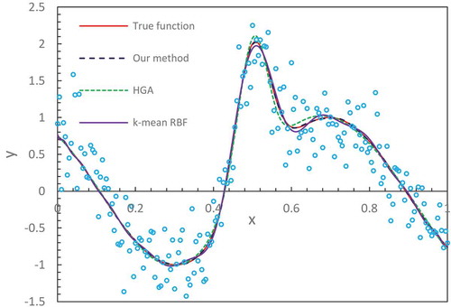
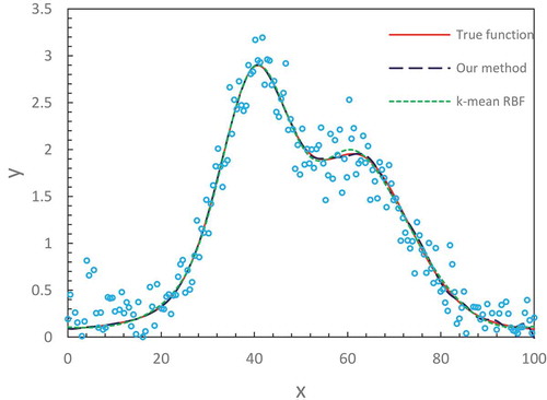
In Figures 1 and 2, we display the true functions as described in Equations (21) and (22(22) ${\mathrm{f}}_2(x)=sin(2(4x-2))+2e^{-16{(4x-2)}^2}x\in \left[0,1\right]$(22) ) and compare the fitting results from different methods. We notice that our method with the number of hidden node M = 32 produces an accurate fitting that nearly overlaps the true functions in the entire domain. The results from the hierarchical genetic algorithm (HGA) (Trejo-Caballero 2015) exhibit a consistent closeness to true function but in individual intervals they slightly deviate from them. The curve from k-mean RBF fitting where the training algorithm of the RBF network is k-mean has slight fluctuations at the region of the lower x-axis position. Table 1 lists the values of the mean-squared errors (MSE) from different methods (Denison, Mallick, and Smith 1998; Trejo-Caballero and Torres-Huitzil 2015). It shows that our estimates are better than others.

Table 1. MSE of various methods for benchmark functions.

	Our method	MCMC	HGA	k-mean RBF
f1(x)	3.2 × 10^−4	7.9 × 10^−3	1.4 × 10^−2	3.4 × 10^−2
f2(x)	1.7 × 10^−4	9.6 × 10^−3	6.7 × 10^−3	1.5 × 10^−2

Figure 1. Comparison of fitting results for benchmark function 1.

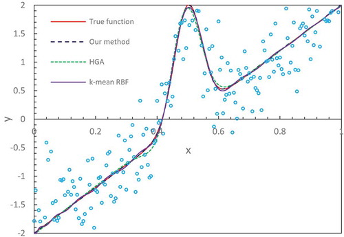
Figure 2. Comparison of fitting results for benchmark function 2.

In Figures 3–5, we illustrate the fitting results for three synthetized spectral datasets. These are challenging fitting tasks because the distorted shape, noise and multiple peaks of curves make them extremely difficult to fit by using a conventional numerical-based method, with which its solution is prone to get trapped in local minima. Our method with the optimized number of hidden nodes (M = 34) obtained satisfactory results for all three spectral lines. They fully capture the characteristics of data distribution matching specific line shape.

Figure 3. Fitting results for Gaussian2 dataset.

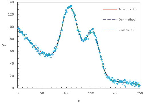
Figure 4.A fitting result for Lorentzian line shape.

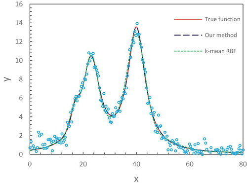
Figure 5.A fitting result for Voigt line shape.

The above two set examples show that our adjusted and optimized ELM with a finite number of neurons well fits various datasets to smooth curves represented by the intrinsic regression functions. The universal approximation theorems by Hornik (1991) and Park and Sandberg (1991) emphasize the sufficiently many neurons at hidden layer to be required for approximating a target function to an arbitrary accuracy. From the viewpoint of practical applications, the implementation of such a concept of sufficiently many neurons actually doesn’t mean a huge number of neurons that must be involved. Instead, no more than 40 neurons are sufficient to perform a nonlinear transformation from input space to output space. Despite the finite number of neurons, each neuron in the hidden layer is characterized with the different values of internal parameters which are randomly assigned by obeying a probabilistic distribution. This creates diverse contributions with the local generalization property. Thus, each distinct contribution comprises a kind of effective approximation in the subspace nearby a center. A superimposition of all the local contributions constructs a global approximation in which fine tuning of individual neuron’s contribution is performed through the output weights in the learning process.

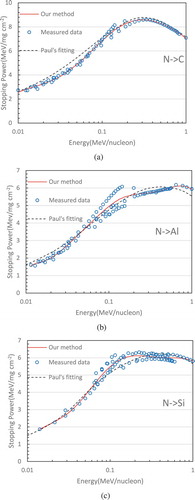
Finally, we wish to show some fitting results for real-world measured data – stopping power curve fitting from high energy physics experiments. The stopping power is defined as a physics quantity of the energy loss per unit distance when the ion beam transverses through solid matter or biological tissues. Stopping power data can be measured experimentally by high energy physics facilities. Accurate knowledge of stopping power curve plays a key role in ion beam analysis (IBA) technique and heavy ion radiation therapy technology for which there are more than 60 particle centers of medical applications in operation around the world for the treatment of various cancers (http://www.health.qld.gov.au/_data/assets/pdf_file/./proton-hvy-ion- therapy.pdf). In IBA, a MeV ion beam is used to probe the elemental composition and its depth distribution near the solid surface layer, where the accuracy of the probe is extremely sensitive to the stopping power data on the projectiles and matter. In heavy ion radiation therapy (such as clinical use of carbon, oxygen and fluorine), the determination of incident ion beam dosimetry highly relies on stopping power data. There are numerous combinations between the projectile ions and target matter elements. We only select oxygen projectiles and nitrogen projectiles incident to the target materials of carbon, aluminum and silicon as investigation examples. As illustrated in Figures 6a–c and 7a–c, our fitting results with using as few as four basis functions are compared with Paul’s empirical fitting (Paul and Schinner 2003), which was based on the pure numerical method. Our results agree with measured points better than Paul’s fitting overall and are better to reflect the trend of data distribution. For example, let us examine the case of oxygen projectiles incident to a carbon target. From Figure 6a, it can be clearly seen that the values of Paul’s fitting at the relatively lower energy region are higher than they should be, while they appear lower than the actual data points at some higher energy positions. Opposite to Figure 6a, in Figure 6c, Paul’s result appears a little low at some middle energy axis positions and a little high in the higher energy region for the case of oxygen projectiles incident on silicon. Similarly, for the cases of nitrogen in the targets carbon, aluminum and silicon, it has been observed that our results are closer to the actual data distribution.

Figure 6. Comparison of fitting results between our method and Paul’s empirical fitting. (a) O→C, (b) O→Al, (c) O→Si.

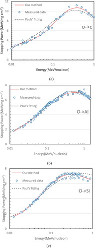
Figure 7. Comparison of fitting results between our method and Paul’s empirical fitting. (a) N→C, (b) N→Al, (c) N→Si.

Conclusion and Future Work

This work proposes a neural network-based technique to resolve one of the traditional numerical analysis problems-curve fitting. This can be recognized as an alternative approach based on intelligent learning to challenge the classical numerical analysis technique. Our method incorporates the advantages of ELM algorithm and the PSO optimization technique. The number of single hidden layer nodes of the network is a key factor to achieve a good generalization, which is optimized by using the PSO method. The architecture of the ELM model is modified by introducing an additional linear neuron to correct the localized behavior of basis functions. Several datasets on benchmark problems and typical spectroscopic line shape data are tested to verify the proposed method. It has been observed that satisfactory accuracies are achieved in various tough fitting tasks. Future work will focus on two aspects: (i) reducing network size by a full optimization for all parameters of the network configuration and (ii) exploring the use of the proposed method in multiple-dimension even sparse data fitting.

Disclosure Statement

I certify that there is no actual or potential conflict of interest in relation to this article.

References

- Bhandari, H. N., X. Ma, A. K. Paul, P. Smith, and W. L. Hase. 2018. PSO method for fitting analytic potential energy functions. Application to I− (H2O). Journal of Chemical Theory and Computation 14:1321–32. doi:10.1021/acs.jctc.7b01122.
- Broomhead, D. S., and D. Lowe. 1988. Multivariable function interpolation and adaptive networks. Complex Systems 2:321–55.
- Denison, D. G. T., B. K. Mallick, and A. F. M. Smith. 1998. Automatic Bayesian curve fitting. Journal of the Royal Statistical Society: Series B (Statistical Methodology) 60 (2):333–50. doi:10.1111/1467-9868.00128.
- Dimatteo, I., C. R. Genovese, and R. E. Kass. 2001. Bayesian curve-fitting with free-knot splines. Biometrika 88 (4):1055–71. doi:10.1093/biomet/88.4.1055.
- Eberhart, R. C., and J. Kennedy. 1995. A new optimizer using particle swarm theory. Proceedings of 6th Int. Symp. Micro Machine and Human Science, 39–43, Nagoya, Japan.
- Eberhart, R. C., P. K. Simpson, and R. W. Dobbin. 1996. Computational intelligence PC tools. Boston: Academic Press.
- Gálvez, A., and A. Iglesias. 2011. Efficient particle swarm optimization approach for data fitting with free knot B-splines. Computer-Aided Design 43:1683–92. doi:10.1016/j.cad.2011.07.010.
- Gulsen, M., A. E. Smith, and D. M. Tate. 1995. A genetic algorithm approach to curve fitting. International Journal of Production Research 33 (7):911–23. doi:10.1080/00207549508904789.
- Hornik, K. 1991. Approximation capabilities of multilayer feedforward networks. Neural Networks 4 (2):251–57. doi:10.1016/0893-6080(91)90009-T.
- Huang, G. B., Q. Y. Zhu, and C. K. Siew. 2006. Extreme learning machine: theory and applications. Neurocomputing 70:489–501. doi:10.1016/j.neucom.2005.12.126.
- Huang, G.-B., H. Zhou, X. Ding, and R. Zhang. 2012. Extreme learning machine for regression and multiclass classification. IEEE Transactions on Systems, Man, and Cybernetics, Part B (Cybernetics) 42 (2):513–29. doi:10.1109/TSMCB.2011.2168604.
- Karr, C. L., B. Weck, D. L. Massart, and P. Vankeerberghen. 1995. Least median squares curve fitting using a genetic algorithm. Engineering Applications of Artificial Intelligence 8 (2):177–89. doi:10.1016/0952-1976(94)00064-T.
- Karr, C. L., D. A. Stanley, and B. J. Scheiner. 1991. Genetic algorithm applied to least squares curve fitting. U.S. Bureau of Mines Report Investigations 9339.
- Leshno, M., V. Y. Lin, A. Pinkus, S. Schocken. 1993. Multilayer feedforward networks with a nonpolynomial activation function can approximate any function. Neural Networks. 6(6):861–67. doi:10.1016/S0893-6080(05)80131-5.
- Li, M., and B. Verma. 2016. Nonlinear curve fitting to stopping power data using RBF neural networks. Expert Systems with Applications 45:161–71. doi:10.1016/j.eswa.2015.09.033.
- Marquardt, D. 1963. An algorithm for the least-squares estimation of nonlinear parameters. SIAM Journal of Applied Mathematics 11 (2):431–41. doi:10.1137/0111030.
- Park, J., and I. W. Sandberg. 1991. Universal approximation using radial basis function networks. Neural Computation 3:246–57. doi:10.1162/neco.1991.3.2.246.
- Paul, H., and A. Schinner. 2003. Empirical stopping power table for ions from 3Li to 18Ar and from 0.001 to 1000 MeV/nucleon in solids and gases. Atomic Data and Nuclear Data Tables 85:377–452. doi:10.1016/j.adt.2003.08.003.
- Serre, D. 2002. Matrices: theory and applications. New York: Springer.
- Shinzawa, H., J. Jiang, M. Iwahashi, and Y. Ozaki. 2007. Robust curve fitting method for optical spectra by least median squares (LMedS) estimator with particle swarm optimization (PSO). Analytical Sciences 23 (7):81–785. doi:10.2116/analsci.23.781.
- Trejo-Caballero, G., and C. Torres-Huitzil. 2015. Automatic curve fitting based on radial basis functions and a hierarchical genetic algorithm. Mathematical Problems in Engineering 14. Article ID 731207.
- Waterfall, J., F. Casey, R. Gutenkunst, K. Brown, C. Myers, P. Browuwer, V. Elser, and J. Sethna. 2006. The sloppy model universality class and the Vandermonde matrix. Physical Review Letters 97:150601–05. doi:10.1103/PhysRevLett.97.150601.
- Yoshimoto, F., T. Harada, and Y. Yoshimoto. 2003. Data fitting with a spline using a real-coded genetic algorithm. Computer-Aided Design 35:751–60. doi:10.1016/S0010-4485(03)00006-X.