Predicting Calorific Value of Thar Lignite Deposit: A Comparison between Back-propagation Neural Networks (BPNN), Gradient Boosting Trees (GBT), and Multiple Linear Regression (MLR)

ABSTRACT

Calorific value provides a strong measure of useful energy during coal utilization. Previously, different AI techniques have been used for the prediction of calorific value; however, one model is not valid for all geographic locations. In this research, Lower Calorific Value (LCV) of the Thar coal region in Pakistan is predicted from proximate analysis of 693 drill holes extending to 9,000 sq. km. Researchers have applied different techniques to produce the best model for prediction of calorific value; however, Gradient Boosting Trees (GBT) has not been used for this purpose. A comparison of GBT, Back-propagation Neural Networks (BPNN), and Multiple Linear Regression (MLR) is presented to predict the calorific value from a total of 8,039 samples with 1 m support interval. The samples were split randomly into 70:15:15 for training, testing, and validation of GBT, BPNN, and MLR models, reporting correlations of 0.90, 0.89, and 0.80, respectively. The features’ importance was reported by the intuitive and best-performing GBT model in decreasing order of importance as: Volatile Matter, Fixed Carbon, Moisture, and Ash with corresponding feature importance values of 0.50, 0.30, 0.12, and 0.08.

Introduction

Lower/Net Calorific Value (Higher/Gross Calorific Value – Latent heat of vaporization of Water) decides the quality of coal and requires constant monitoring during operations of a power plant (Kumari et al. 2019). A combination of prediction models can be coupled with sensors to create model-driven soft sensors for this job that can give input for real-time monitoring and optimization of the plant performance (Belkhir and Frey 2016). Various empirical (Kumari et al. 2019), statistical (Akhtar, Sheikh, and Munir 2017; Akkaya 2009), and artificial intelligence-based algorithms, e.g. Neural Network algorithms (Açikkar and Sivrikaya 2018; Chelgani, Mesroghli, and Hower 2010; Erik and Yilmaz 2011; Feng et al. 2015; Mesroghli, Jorjani, and Chelgani 2009; Wen, Jian, and Wang 2017; Yilmaz, Erik, and Kaynar 2010); Support Vector Machines (Tan et al. 2015); Random Forest (Matin and Chehreh Chelgani 2016); and Adaptive Neuro-Fuzzy Inference Systems (Erik and Yilmaz 2011), have been used to predict the calorific value. However, researchers agree on the development of separate calorific value prediction model for different regions (Tan et al. 2015). These models use input variables from proximate analyses (Açikkar and Sivrikaya 2018; Akhtar, Sheikh, and Munir 2017; Akkaya 2009; Feng et al. 2015; Tan et al. 2015) or ultimate analyses (Yilmaz, Erik, and Kaynar 2010) or combination of both (Chelgani, Mesroghli, and Hower 2010; Erik and Yilmaz 2011; Matin and Chehreh Chelgani 2016; Mesroghli, Jorjani, and Chelgani 2009; Wen, Jian, and Wang 2017). The majority of these studies suggest that models perform better having input variables defined by ultimate analyses (Açikkar and Sivrikaya 2018; Akhtar, Sheikh, and Munir 2017; Akkaya 2009; Feng et al. 2015; Tan et al. 2015; Yilmaz, Erik, and Kaynar 2010) or a combination of ultimate + proximate analyses (Chelgani, Mesroghli, and Hower 2010; Erik and Yilmaz 2011; Matin and Chehreh Chelgani 2016; Mesroghli, Jorjani, and Chelgani 2009; Wen, Jian, and Wang 2017). However, acquiring ultimate analyses requires specialized lab equipment and is, therefore, time consuming and costly. Calorific value prediction models using proximate analyses will be beneficial, especially with the emergence of online sensors for proximate analyses (Klein 2008; Snider, Evans, and Woodward 2001; RealTimeInstruments 2019). Gradient Boosting Trees (GBT), in contrast to ANN, is intuitive, has a lesser number of hyper-parameters, and has not been applied to predict the calorific value of coal. GBT is very powerful in capturing complex relationships (Makhotin, Koroteev, and Burnaev 2019; Nolan, Fienen, and Lorenz 2015; Patri and Patnaik 2015; Zhou et al. 2016), efficient non-linear function mappings, and better generalization (Abiodun et al. 2018; Asadi 2017; Makhotin, Koroteev, and Burnaev 2019; Nolan, Fienen, and Lorenz 2015; Patri and Patnaik 2015; Zhou et al. 2016). This paper compares the traditional statistical model (Multiple Linear Regression (MLR)) with GBT and Back-propagation neural network (BPNN) models’ performance for prediction of lower calorific value (LCV) from proximate analyses of recently explored Thar coalfield (consisting of 12 regional blocks). In the next section, a background of GBT and Artificial Neural Network (ANN) is presented. Thar coalfield dataset is presented next, followed by a methodology section. Then, the results and discussion section is presented, followed by a final conclusion section.

Back-Propagation Neural Network (BPNN)

BPNN is a supervised learning algorithm and a class of ANNs that uses back-propagation for the training of network. ANN consists of input layer, hidden layer/s, and output layer (Goodfellow, Yoshua, and Aaron 2016; Gulli and Pal 2018; Russell and Norvig 2001). Every layer has nodes; the input layer and output layer have total number of nodes equal to the number of input features and output features, respectively, while the total number of hidden layers and nodes can vary. Connections between nodes are represented by weights; the input value to a node in any layer between the second and the output layer is weighed linear combination of outputs (activation function) from the nodes in the preceding layer. The output of a node is derived by feeding this value to an activation function in every node (Goodfellow, Yoshua, and Aaron 2016; Gulli and Pal 2018; Russell and Norvig 2001). Activation function adds nonlinearity and makes ANN a universal approximator (Goodfellow, Yoshua, and Aaron 2016; Gulli and Pal 2018; Russell and Norvig 2001). Different activation functions like sigmoid, tanh, and relu could be used for adding nonlinearity and making ANN robust in approximating complex processes. The main task in an ANN is to learn connections/weights through different techniques, such as the most widely used back-propagation (Goodfellow, Yoshua, and Aaron 2016; Gulli and Pal 2018; Russell and Norvig 2001). Learning through back-propagation involves backward adjustment of weights by propagating the error from the output to the input layer. This is an iterative process where optimization techniques gradually decrease the error in the model at each step/iteration/epoch (Goodfellow, Yoshua, and Aaron 2016; Gulli and Pal 2018; Russell and Norvig 2001; Wythoff 1993). Distribution of error minimizes the objective function which is a measure of the difference between actual outputs of given data and the reported output from the model. Back-propagation is carried out using various optimization techniques like gradient descent, RMSProp, and Adam optimization.

Tuning a Neural Network

Various parameters are tuned to obtain a better model that is a representation of the whole population rather than only the training data. A higher number of hidden layers and nodes add complexity to the model, increasing over-fitting (i.e. increasing error metric at the validation stage) (Goodfellow, Yoshua, and Aaron 2016; Gulli and Pal 2018; Nazzal, El-emary, and Najim 2008; Russell and Norvig 2001). The Relu activation function has greater computational efficiency compared to other activation functions (Goodfellow, Yoshua, and Aaron 2016; Gulli and Pal 2018). Different regularization techniques (L1/L2/dropout, etc.) are available; the L1/L2 regularization techniques penalize higher weights, whereas dropout technique randomly switches off certain percent of the nodes in a layer (Goodfellow, Yoshua, and Aaron 2016; Gulli and Pal 2018; Rychetsky, Ortmann, and Glesner 1998). Batch size, i.e. samples fed to a network for learning at each step, if kept low, would lead to memory and computational efficiency but less accuracy and erratic training (Goodfellow, Yoshua, and Aaron 2016; Gulli and Pal 2018; Radiuk 2017). Usually, Adam optimization technique is fast and provides better convergence results (Bock, Goppold, and Martin 2018; Goodfellow, Yoshua, and Aaron 2016; Gulli and Pal 2018; Kingma and Jimmy 2014, 2014) among other choices of optimization techniques like gradient descent (Ghasemalizadeh, Khaleghian, and Taheri 2016; Goodfellow, Yoshua, and Aaron 2016; Gulli and Pal 2018). Selection of parameters of optimizer, e.g. learning rate and momentum, are parameters that require tuning to improve model performance. Learning rate and momentum of optimizer is tuned to identify the global optimum instead of being stuck in the local optimum.

Gradient Boosting Trees (GBT)

GBT is composed of a number of decision trees. Decision Tree is a supervised learning algorithm in which the main task is to construct tree-like architecture from the given data. Tree has root node, intermediate nodes, and leaf nodes drawn upside down with its root at the top and leaf at its bottom. Root node is the best attribute of whole data, intermediate nodes represent best attributes of subsets of data, and leaf nodes represent the output attributes (Russell and Norvig 2001; Trevor, Tibshiran, and Friedman 2009). In other words, whole tree construction is about finding the best attribute of data and dividing data into subsets of data sequentially (see figure 1). Different algorithms like Iterative Dichotomiser 3 (ID3) or Classification and Regression Trees (CART) are used for finding this best attribute (Russell and Norvig 2001; Trevor, Tibshiran, and Friedman 2009). In ID3, at each stage, all the input attributes are paired with the output attributes; the best input attribute among all is the one that shows greater homogeneity of the output attribute. Information gain (in case of classification) or mean-square-error/standard deviation (in case of regression) is used for measuring homogeneity (Russell and Norvig 2001; Trevor, Tibshiran, and Friedman 2009). In regression, the first step, mean-square-error/standard deviation of target/output variable/attribute is calculated for the complete dataset.

$S=\sqrt{\frac{{\sum (x-\bar{x})}^2}{n}}$

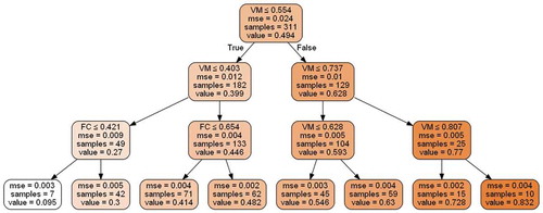
Figure 1. Decision tree having depth-4

where S is standard deviation of output/target variable for complete dataset,

x is output/target variable,

x̅ is mean of output/target variable,

and n is total number of samples.

In the second step, the best attribute is chosen by splitting the dataset into a number of subsets equal to the number of the input attributes such that each subset contains one input attribute and corresponding output attribute. The standard deviation for each subset is calculated:

$S(T,X)=\sum _{c\in X}P(c)S(c)$

where T is target variable,

X is input variable and

c is the cth class defined by a range of values of an input variable.

P(c) is probability associated with class c of the input variable.

S(c) is standard deviation of target variable associated with class c of the input variable.

The resulting standard deviation of each subset is subtracted from standard deviation of dataset before split to find standard deviation reduction value for each subset.

$SDR(T,X)=S(T)-S(T,X)$

The best subset/input attribute among all is the one that gives maximum standard deviation reduction value (Russell and Norvig 2001; Trevor, Tibshiran, and Friedman 2009). The best input attribute value found is placed as a root node and the dataset is divided into subsets equal to the number of classes (different range values) of that best attribute. This process is repeated for each subset of data from which the next splitting attributes are selected as intermediate nodes in hierarchical order. These next best attributes will be placed as child nodes below the previous nodes in a tree-like architecture. This process continues until all data are processed or some criterion/criteria are met. Some of the criteria used for stopping this process are depth of tree, minimum samples at leaf nodes, and threshold of a performance metric (Russell and Norvig 2001; Trevor, Tibshiran, and Friedman 2009). In the end nodes, where process stops are called leaf nodes, which represent the classes’ value of the required output attribute. The branches/intermediate nodes in a decision tree represent various possible known outcomes obtained by asking the question on the node. Once the tree is made, to know the output for given situation/input attributes, a query to the root node leads through the branches/intermediate nodes in a tree to the leaf node as the predicted final output (Russell and Norvig 2001; Trevor, Tibshiran, and Friedman 2009). Figure 1 shows decision tree made for LCV prediction of block11 (311 samples) based on proximate analyses data.

Each box in Figure 1 represents a subset of dataset from top to bottom: Best Input Attribute and Its Values in that Subset; Mean Square Error for that Subset; Number of Samples in that Subset and LCV (values are optionally normalized here) as output variable in that Subset.

Decision Tree depicted in Figure 1 is having a depth of four levels, i.e. root node was placed at level1 and leaf nodes placed at level4. Level2 and level3 have all intermediate nodes. At level1, the best attribute selected was volatile matter (VM), and based on the values of VM, two subsets were created for level2. At level2, the best attribute selected for both subsets was again VM. Based on the values of VM in both subsets at level2, further splitting was done into four subsets for level3. At level3, fixed carbon (FC) was chosen as the best attribute for two subsets where VM was chosen as best for the other two subsets. Based on their values in respective subsets, the dataset was further split into eight subsets for leaf nodes/level4.

As seen from Figure 1, VM is the most important feature for predicting LCV, followed by FC, whereas ash and moisture are insignificant. Therefore, decision tree is intuitive in explaining feature importance; however, it suffers from a high chance of overfitting and relatively lower validation accuracy (Russell and Norvig 2001; Trevor, Tibshiran, and Friedman 2009). Some of the strategies for better generalization and reduction in overfitting includes pre-pruning, i.e. stopping the growth of tree by defining a threshold before it perfectly classifies the data (i.e. decreasing depth), increasing the number of samples used in the calculation of homogeneity of samples, using lesser number of variables in case of too many variables, and use of ensemble methods (Trevor, Tibshiran, and Friedman 2009; Russell and Norvig 200; McSherry 1999). Ensemble methods combine multiple algorithms (decision trees in this case) to make a more generalized algorithm. These methods have base learners (decision trees in this case) and a procedure for combining those base learners. Procedures for combining base learners include bagging and boosting. In bagging, different base learners (decision trees here) are developed using randomly resampled dataset with/without replacement. The output of bagging is calculated by taking the average of all base learners and the algorithm is called Random Forest (Russell and Norvig 2001; Trevor, Tibshiran, and Friedman 2009). Boosting, on the other hand, first trains a single base learner, next another base learner is trained; however, this time samples that were learned poorly by the previous learner are given more weight, and the process continues till the maximum limit for the number of base learners is met. In boosting, prediction is made for all learners/trees; the predicted value is weighed combination according to the performance of each learner on training data. In this way, weak base learners combine to make strong learners (Natekin and Knoll 2013; Russell and Norvig 2001; Trevor, Tibshiran, and Friedman 2009). GBT is an ensemble boosting method in which decision tree acts as a base learner sequentially arranged in a hierarchy one after the other (Natekin and Knoll 2013; Russell and Norvig 2001; Trevor, Tibshiran, and Friedman 2009). Initially for building the first (top) decision tree, each sample is equally weighed, but for other trees in the hierarchy, the samples are weighed according to their performance. Samples with lower mean error are weighed less for the next tree, while samples with higher prediction error are weighed more. In such a way, all samples are learned equally well resulting in a reduction in overfitting (Natekin and Knoll 2013; Russell and Norvig 2001; Trevor, Tibshiran, and Friedman 2009). The number of decision trees and learning rate are two important hyper-parameters (Natekin and Knoll 2013; Russell and Norvig 2001; Trevor, Tibshiran, and Friedman 2009). Higher learning rate means lesser number of trees is needed and vice versa. Generally, lower learning rate and large number of trees are used in models where there are chances of higher overfitting.

Thar Coalfield Location and Dataset

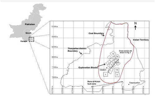
Thar coalfield is located in the eastern part of Sindh Province (shown in Figure 2) of Pakistan containing 175 billion tons lignite resources (Singh, Atkins, and Pathan 2010) between 130 and 250 m depth in 9000 km² area.

Figure 2. Location map of Thar Lignite Field, Pakistan

The data used in this study are obtained from 12 different blocks explored in Thar coalfield of Pakistan from 1994 to 2012.

A total of 6,095 samples, through 693 drill holes (please see Figure 3) from 12 blocks (please see Table 1), were reported for LCV and proximate analyses (moisture, ash, FC, VM) on as-received basis.

Table 1. Summary of drilling activities

	No. of drillholes	Average dillhole spacing (m)	Total drilled meters (m)	Minimum depth (m)	Maximum depth (m)	Average drillhole depth (m)
All 12 blocks	693	1,400	166,675	109.78	319.68	240.51

Figure 3. Location of drill holes in Easting-Northing

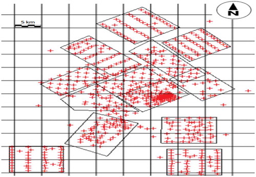
Samples were composited to 1-m support/core interval resulting in a total of 8,039 samples, each having 1-m thickness approximately.

Table 2 shows descriptive statistics including minimum, maximum, mean, and standard deviation for all variables of 8,039 samples.

Table 2. Descriptive statistics for 8,039 samples

8,039 samples	Mean	Std dev	Min	Max
Ash	6.83	4.20	1.06	47.51
FC	19.32	4.03	3.5	41.46
Moisture	47.4	5.50	9.41	68.58
VM	26.45	4.51	7.95	52.84
Cal V	2,897	403	536.23	5,277.97

Predicting Calorific Value of Thar Coal Deposit

In this study, the hold out validation method was used and the correlation coefficient was chosen as a performance metric. Data were first normalized (having values between range [0–1]), split randomly into three parts 70:15:15 for training, testing/tuning, and validation, respectively.

For both BPNN and GBT, ranges of hyper-parameter values were explored in grid search manner between the extreme values given in Tables 3 and 4, respectively. In both cases, models fitted on extreme end values of respective ranges of hyper-parameters either under-fitted or over-fitted the model, suggesting a domain of search to produce good results.

Table 3. BPNN hyper-parameters ranges to be searched

Hyper-parameters	Range	Hyper-parameters	Range
Number of Layers	2–6	Nodes/Layer	100–300
Activation functions	sigmoid/tanh/relu	Batch size	10–4,000
Regularization L2	0.001 to 5	Momentum	0.5 to 0.999
Regularization dropout	10–50%	Data preprocessing	Standardization/ Normalization
Learning Rate Alpha	0.001 to 0.5
Optimizer	Gradient Descent/Adam	Weight initialization Strategy and range	Uniform/Normal (−1 to 1)/(0 to 1)/(−6 to 6)

Regularization L2 values searched from 0.001 to 5 such that (Next L2 value = previous L2 value + 0.1).

Regularization dropout values searched from 10% to 50% with increment of 5%.

Learning Rate (Alpha) values searched from 0.001 to 0.5 such that (Next Alpha = previous Alpha + 0.01).

Nodes/Layer values from 100 to 300 searched with increment of 50.

Batch size value searched from 10 to 4,000 with increment of 200.

Momentum values searched from 0.5 to 0.999 with increment of 0.1.

Table 4. GBT hyper-parameters ranges to be searched

Hyper-parameters	Range	Hyper-parameters	Range
Number of decision trees	50 to 10,000	Minimum samples at leaf node	50–100%
Learning Rate Alpha	0.001 to 0.3	Batch size	10–99% samples for split

Number of decision trees searched from 50 to 10,000 with increment of 100.

Learning Rate Alpha searched from 0.001 to 0.3 such that (Next Alpha = Previous Alpha + 0.01).

Minimum samples at leaf node searched from 50% to 100% with increment of 5%.

Batch size searched from 10% to 99% with increment of 5%.

The analysis was done using python libraries like Numpy and Pandas where visualization and interactive 3D visualization was done using Matplotlib/Seaborn and Plotly, respectively. BPNN was applied using Tensorflow and GBT was applied using Python Scikit-learn library.

Results and Discussion

In BPNN, an increasing number of hidden layers, neurons, and a decrease in regularization values resulted in an increase in correlation during the training phase (0.95) and a decrease in correlation during the testing phase (0.5). Higher learning rate and lower batch sizes made BPNN erratic and were therefore difficult to converge. The use of higher momentum values in combination with Relu activation function, and Adam optimizer made BPNN fast and helped reach global optima instead of getting stuck in the local optima. Varying weight initialization and data pre-processing technique did not have any effect on the results. Optimum parameters after tuning are presented in Table 5.

Table 5. Optimum hyper-parameters for BPNN

Hyper-parameters	Value	Hyper-parameters	Range
Number of Layers	4	Nodes/Layer	200
Activation functions	Relu	Batch size	200
Regularization L2	0.3	Momentum	0.9
Regularization dropout	20%	Data preprocessing	Normalization
Learning Rate Alpha	0.05
Optimizer	Adam	Weight initialization Strategy and range	Uniform (−1 to 1)

For GBT, the decrease in number of trees, higher learning rate, lower value of minimum samples at leaf node, and decreasing batch size resulted in a correlation of 0.99 during training phase and a correlation of 0.55 during testing phase. Optimum parameters after tuning are presented in Table 6.

Table 6. Optimum hyper-parameters for GBT

Hyper-parameters	Value	Hyper-parameters	Value
Number of decision trees	3000	Minimum samples at leaf node	70%
Learning Rate Alpha	0.001	Batch size	90% samples for split

The relationship between LCV and proximate analysis in Thar region is nonlinear as shown in Table 7 where MLR (correlation = 0.8) performance was lower compared to BPNN (correlation = 0.89) and GBT (correlation = 0.90) models. GBT and BPNN perform equally well; however, intuitiveness of GBT model makes it more attractive than BPNN. Feature importance computed during GBT was reported to be 0.50, 0.30, 0.12, and 0.08 for VM, FC, moisture, and ash, respectively. This suggests the importance of VM in the Thar region for LCV prediction. The results are in conformity with the lignite coal resource having higher VM and moisture content, and lower carbon content. Correlation will likely improve significantly once production data are available for each block.

Table 7. Machine learning algorithms results for global data

		Hold out
No. of Samples	Model Name	Train	Test	Val
8,039	BPNN	0.92	0.89	0.89
	GBT	0.94	0.91	0.90
	MLR	0.85	0.80	0.80

Conclusions

This paper predicts the LCV of Thar coalfield using proximate analyses parameters. All four proximate analyses parameters were used to predict LCV using BPNN, GBT, and MLR. GBT model performed better during LCV prediction of Thar coal region in Pakistan with correlation = 0.90 compared to BPNN (correlation = 0.89) and MLR (correlation = 0.80). The intuitiveness of GBT model also enabled to identify the most important feature of LCV as VM. The prediction model represents the relationship between proximate and LCV for a wide Thar region. Model correlations are likely to improve at block level when production data from these blocks are obtained during the mining phase.

Acknowledgments

The funding for this work was provided by the Higher Education Commission of Pakistan.

References

- Abiodun, O. I., A. Jantan, A. E. Omolara, K. V. Dada, N. A. E. Mohamed, and H. Arshad. 2018. State-of-the-art in artificial neural network applications: a survey. Heliyon 4 (11):e00938. doi:10.1016/j.heliyon.2018.e00938.
- Açikkar, M., and O. Sivrikaya. 2018. Prediction of gross calorific value of coal based on proximate analysis using multiple linear regression and artificial neural networks. Turkish Journal of Electrical Engineering and Computer Sciences 26 (5):2541–52. doi:10.3906/elk-1802-50.
- Akhtar, J., N. Sheikh, and S. Munir. 2017. Linear regression-based correlations for estimation of high heating values of Pakistani lignite coals. Energy Sources, Part A: Recovery, Utilization and Environmental Effects 39 (10):1063–70. doi:10.1080/15567036.2017.1289283.
- Akkaya, A. V. 2009. Proximate analysis based multiple regression models for higher heating value estimation of low rank coals. Fuel Processing Technology 90 (2):165–70. doi:10.1016/j.fuproc.2008.08.016.
- Asadi, A. 2017. Application of artificial neural networks in prediction of uniaxial compressive strength of rocks using well logs and drilling data. Procedia Engineering 191:279–86. doi:10.1016/j.proeng.2017.05.182.
- Belkhir, F., and G. Frey. 2016. Model-driven soft sensor for predicting biomass calorific value in combustion power plants. IEEE 11th Conference on Industrial Electronics and Applications (ICIEA), Hefei, pp. 807–12. doi: 10.1109/ICIEA.2016.7603692
- Bock, S., J. Goppold, and W. Martin. 2018. An improvement of the convergence proof of the ADAM-optimizer. 1–5. http://arxiv.org/abs/1804.10587.
- Chelgani, S., C. S. Mesroghli, and J. C. Hower. 2010. Simultaneous prediction of coal rank parameters based on ultimate analysis using regression and artificial neural network. International Journal of Coal Geology 83 (1):31–34. doi:10.1016/j.coal.2010.03.004.
- Erik, N. Y., and I. Yilmaz. 2011. On the use of conventional and soft computing models for prediction of gross calorific value (GCV) of coal. International Journal of Coal Preparation and Utilization 31 (1):32–59. doi:10.1080/19392699.2010.534683.
- Feng, Q., J. Zhang, X. Zhang, and S. Wen. 2015. Proximate analysis based prediction of gross calorific value of coals: a comparison of support vector machine, alternating conditional expectation and artificial neural network. Fuel Processing Technology 129:120–29. doi:10.1016/j.fuproc.2014.09.001.
- Ghasemalizadeh, O., S. Khaleghian, and S. Taheri. 2016. A review of optimization techniques in artificial networks. International Journal of Advanced Research 4 (9):1668–86. doi:10.21474/ijar01/1627.
- Goodfellow, I., B. Yoshua, and C. Aaron. 2016. Deep learning. MIT Press. https://doi.org/10.1038/nmeth.3707.
- Gulli, A., and S. Pal. 2018. Deep learning with Keras. Birmingham, UK: Packt Publishing.
- Kingma, D. P., and B. Jimmy 2014. Adam: A method for stochastic optimization. 1–15. http://arxiv.org/abs/1412.6980.
- Klein, A. 2008. Online X-ray elemental analysis of coal to determine ash, sulphur, calorific value and volatiles. Indutech Instruments GmbH. Simmersfeld, Germany.
- Kumari, P., A. K. Singh, D. A. Wood, and B. Hazra. 2019. Predictions of gross calorific value of indian coals from their moisture and ash content. Journal of the Geological Society of India 93 (4):437–42. doi:10.1007/s12594-019-1198-5.
- Makhotin, I., D. Koroteev, and E. Burnaev. 2019. Gradient boosting to boost the efficiency of hydraulic fracturing. Journal of Petroleum Exploration and Production Technology 0 (0):0. doi:10.1007/s13202-019-0636-7.
- Matin, S. S., and S. Chehreh Chelgani. 2016. Estimation of coal gross calorific value based on various analyses by random forest method. Fuel 177:274–78. doi:10.1016/j.fuel.2016.03.031.
- McSherry, D. 1999. Strategic induction of decision trees BT – research and development in expert systems XV. Research and Development in Expert Systems XV, No. Chapter 2:15–26. doi:10.1023/A:1022643204877.
- Mesroghli, S., E. Jorjani, and S. C. Chelgani. 2009. Estimation of gross calorific value based on coal analysis using regression and artificial neural networks. International Journal of Coal Geology 79 (1–2):49–54. doi:10.1016/j.coal.2009.04.002.
- Natekin, A., and A. Knoll. 2013. Gradient boosting machines, a tutorial. Frontiers in Neurorobotics 7 (Dec). doi: 10.3389/fnbot.2013.00021.
- Nazzal, J. M., I. M. El-emary, and S. A. Najim. 2008. Multilayer perceptron neural network (MLPs). World Applied Sciences Journal 5 (5):546–52.
- Nolan, B. T., M. N. Fienen, and D. L. Lorenz. 2015. A statistical learning framework for groundwater nitrate models of the central valley, California, USA. Journal of Hydrology 531:902–11. doi:10.1016/j.jhydrol.2015.10.025.
- Patri, A., and Y. Patnaik. 2015. Random forest and stochastic gradient tree boosting based approach for the prediction of airfoil self-noise. Procedia Computer Science 46 (Icict 2014):109–21. doi:10.1016/j.procs.2015.02.001.
- Radiuk, P. M. 2017. Impact of training set batch size on the performance of convolutional neural networks for diverse datasets. Information Technology and Management Science 20(1):20–24. doi:10.1515/itms-2017-0003.
- RealTimeInstruments. 2019. Online analyzers used in coal. Accessed August 20, 2019. http://www.realtimegrp.com/real-time-instrument/coal-power/coal-and-power/.
- Russell, S. J., and P. Norvig. 2001. Artificial intelligence: A modern approach. Harlow, England: Prentice Hall.
- Rychetsky, M., S. Ortmann, and M. Glesner 1998. Pruning and regularization techniques for feed forward nets applied on a real world data base. International Symposium on Neural Computation, 603–09. Vienna, Austria.
- Singh, R. N., A. S. Atkins, and A. G. Pathan. 2010. Water resources assessment associated with lignite operations in Thar, Sindh, Pakistan. Archives of Mining Sciences 55:425–40.
- Snider, K., M. Evans, and R. Woodward. 2001. Using an on-line elemental coal analyzer. Hunter Coal Gen Paper, 1–10.
- Sowerby, B. D., C. S. Lim, D. A. Abernethy, Y. Liu, and P. A. Maguire. 1997. On-conveyor belt determination of ash in coal. Menai NSW, Australia: Commonwealth Scientific and Industrial Research Organisation (CSIRO).
- Tan, P., C. Zhang, J. Xia, Q. Y. Fang, and G. Chen. 2015. Estimation of higher heating value of coal based on proximate analysis using support vector regression. Fuel Processing Technology 138:298–304. doi:10.1016/j.fuproc.2015.06.013.
- Trevor, H., R. Tibshiran, and J. Friedman. 2009. Elements of statistical learning. 2nd ed. New York, USA: Springer Series in Statistics.
- Wen, X., S. Jian, and J. Wang. 2017. Prediction models of calorific value of coal based on wavelet neural networks. Fuel 199:512–22. doi:10.1016/j.fuel.2017.03.012.
- Wythoff, B. J. 1993. Backpropagation neural networks a tutorial. Elsevier Science Publishers 18:115–55.
- Yilmaz, I., N. Y. Erik, and O. Kaynar. 2010. Different types of learning algorithms of artificial neural network (ANN) models for prediction of gross calorific value (GCV) of coals. Scientific Research and Essays 5 (16):2242–49.
- ZHOU, J., X. Z. Shi, R. D. Huang, X. Y. Qiu, and C. Chen. 2016. Feasibility of stochastic gradient boosting approach for predicting rockburst damage in burst-prone mines. Transactions of Nonferrous Metals Society of China (English Edition) 26 (7):1938–45. doi:10.1016/S1003-6326(16)64312-1.