A Multi-objective Particle Swarm Optimization Based on Pareto Archive for Integrated Production and Distribution Planning in A Green Supply Chain

ABSTRACT

This paper presents a bi-objective model for integrated production and distribution planning in a multi-period multi-product green supply chain. This paper considers many near-real-world factors, such as: normal and overtime production shifts, limited storage capacity of the finished product and raw materials, different vehicle types, direct and indirect shipping along with considering different production methods that influence the production costs and sale prices, simultaneously. Mixed integer programming model is proposed in which the profit maximization and the CO₂ emission minimization are formulated. A particle swarm optimization algorithm based on Pareto archive that utilizes the genetic algorithm operators is proposed to solve the model.

Introduction

Traditionally, it was believed that different components of the supply chain can be planned independently and in separate directions; however, this point of view leads to the reduction of profit of the system as a whole (Barbarosoğlu and Özgür 1999). Whereas, nowadays the integration of the production and distribution activities can provide competitive advantages by influencing the profitability of the supply chain (Fahimnia et al. 2013).

In green supply chain, the ‘green’ concept refers to considering the effects and relation of the supply chain management and the environment (Srivastava 2007). Also, with respect to global warming which is a direct result of human activities since the industrial revolution, the emission of greenhouse gases must be considered in coordinated activities of supply chains. The most important greenhouse gas produced by human activities is CO₂, such that between years 1970–2004 increased by 80%, due to the increase in fossil fuels consumption (Sadrnia et al. 2013).

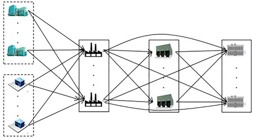
With respect to the importance of integrating production and distribution planning (p-d planning) and considering environmental factors, in this study, a new bi-objective model for the integrated p-d planning problem that simultaneously maximizes profit and minimizes CO₂ emission, in a four-echelon, multi-period, and multi-product supply chain is presented. Raw materials are sent from the suppliers to the factories and the finished products are shipped to the customers either directly or by the means of distribution centers. Furthermore, numerous near-real-world assumptions are taken into account. In addition to revenue from the sale of the finished products, some cost factors including raw material procurement cost, production cost, raw material, and finished products holding cost, transportation, and shortage costs are considered in the model. This mid-term planning model helps the supply chain to look beyond the profit aspect and the right choice of type and number of appropriate vehicles with respect to their amount of greenhouse gas emission, reduces the amount of CO₂ emission.

The remaining paper is organized as follows. Section 2 reviews the related literature. Section 3 gives the general problem definition and the proposed mathematical model. The multi-objective Pareto archive-based particle swarm optimization (PSO) algorithm (named as pa-PSO) is explained in section 4. Section 5 deals with the comparison between pa-PSO and NSGA-II algorithm on the sample problems and case study. Finally, section 6 concludes the paper and suggests some area for future research.

Literature Review

Integrated p-d planning in the area of supply chain management has attracted many attentions in recent years. Sarmiento and Nagi (1999) and Fahimnia et al. (2013)reviewed the p-d planning papers. Srivastava (2007)and Dekker, Bloemhof, and Mallidis (2012) presented review papers on green supply chain management.

In this section, for the abbreviation, the more related multi-objective models of the integrated p-d planning in the supply chain and green supply chain are reviewed. Sadrnia et al. (2013) presented a model for a single period automobile supply chain with two objectives of cost and CO₂ emission minimization and solved the model by the multi-objective gravitational search algorithm. Their model does not account for the shortage costs, normal time and overtime production and direct shipping. Guillén-Gosálbez and Grossmann (2009) studied a stochastic planning model in a liquid products three-echelon supply chain with the objectives of cost and environmental damage minimization. To solve the model, they decomposed the problem into two sub-problems. Guillén-Gosálbez and Grossmann (2010)developed the former works and utilized the ε-constraint and a new branch and bound method. Both articles, do not consider different types of vehicles, direct shipping and shortage decisions. Memari, Rahim, and Ahmad (2015)presented a model in three-echelon green supply chain. They seek to minimize their costs and CO₂ emission through just-in-time shipping. A multi-objective genetic algorithm (GA) and the goal programming approach are used to solve the model. Different types of vehicles, direct shipping, several suppliers, and related decisions are not taken into account. Sarrafha et al. (2015)presented a model for a supply chain with the objectives of cost and average tardiness minimization and solved it with an optimization approach based on the biogeography, multi-objective simulates annealing and NSGA-II algorithms. Moncayo-Martínez and Zhang (2011) presented a model for a three-echelon supply chain that minimizes the cost and lead time. They solved their model by an ant colony optimization algorithm. Mastrocinque et al. (2013)solved the model of Moncayo-Martínez and Zhang (2011) with Bees algorithm. Mirzapour Al-E-Hashem et al. (2011) developed a model for a two-echelon supply chain and considered the cost and demand fluctuation as the stochastic variables. The objectives are minimization of the cost and its variance along with the maximization of the staff productivity. Mirzapour Al-E-Hashem, Malekly, and Aryanezhad (2011) presented a three-echelon supply chain model that considers demand uncertainty. The objectives are minimization of the cost and maximum shortage of all periods. Liu and Papageorgiou (2013)studied a model with three objectives in a two-echelon global supply chain for the process industry.Gholamian, Mahdavi, and Tavakkoli-Moghaddam (2016)modeled a three-echelon supply chain as a non-linear fuzzy four-objective model under uncertainty. Pasandideh, Niaki, and Asadi (2015b) developed a model minimizing the cost and maximizing the average number of sent products. Also Pasandideh, Niaki, and Asadi (2015a) presented another optimization model for a three-echelon supply chain that minimizes the expected and variance of total cost and solved the model with NSGA-II algorithm.

According to the gap of literature review, this paper presents a multi-product and multi-period four-echelon integrated p-d planning model considering several suppliers, factories, customers, distribution centers, transportation routes and vehicles, and environmental factors not studied yet.

Problem Definition

Decorative stones are a group of stones that are cut into specific sizes. In order to produce plaque stone (used in construction sites), rock stones (blocks) are cut into pre-specified thicknesses and then burnished such that the surface becomes totally reflective and smooth. In stone processing industry, many different factors such as color, design, and streak which the raw material might contain make the production and distribution activities difficult. Paying attention to these issues, proposing an appropriate model for the integrated p-d planning of a stone supply chain that considers most of the real-world factors, helps the industry to plan better and more accurate.

Assumptions

• There are a number of type-1 and type-2 raw material suppliers, stone-cutting factories, distribution centers, and customers.

• Transporting the products from factories to the customers can be made by direct and indirect shipments.

• Various products (plaque stones) are produced in factories in normal and overtime shifts.

• There are two production methods. The first method refers to the production using common cutting machines with a lower price level and production cost than the second method in which the high precision cutting machines are utilized.

• Production capacity is limited.

• The limited capacity exists in the supplying the raw material by the suppliers, storing type-1 raw material in the plant, storing finished products in the factory and distribution centers.

• The initial inventory for the first period is considered to be zero.

• Different types of vehicles (e.g. trucks, trailers, train …) exist in all distribution routes.

• Shortage is considered as lost sales.

• Minimum demand in the planning horizon should be satisfied.

Figure 1 shows an overview of the studied supply chain.

Figure 1. An overview of the studied supply chain

Indices

h: Type-1 raw material suppliers

s: Type-2 raw material suppliers

i: Factories

j: Distribution centers (DCs)

c: Customers

p:Products

t: Time periods

$\text{user}o$: Production shift; equals to 1 when production occurs in normal time and when production occurs in overtime

$\text{user}r$: Production method; equals to 1 when normal method is used, and 2 when high precision method is used

$\text{user}l$: Type-1 raw material

$\text{user}u$: Type-2 raw material

$\text{user}TK$: Vehicles between type-1 raw material suppliers and factories

$\text{user}TS$: Vehicles between type-2 raw material suppliers and factories

$\text{user}TD$: Vehicles between DCs and customers

$\text{user}TC$: Vehicles between factories and customers, and between factories and DCs.

Parameters

${\mathbf{d}}_{\mathbf{p}\mathbf{c}\mathbf{t}}$: Demand of product $p$from customer $\text{user}c$ in period $\text{user}t$

${\mathbf{p}}_{\mathbf{p}\mathbf{r}\mathbf{c}}$: Sale price of product $p$produced by method $\text{user}r$ for customer $\text{user}c$

$\mathbf{c}\mathbf{a}{\mathbf{k}}_{\mathbf{l}\mathbf{h}\mathbf{t}}$: Supply capacity of raw material $\text{user}l$ from supplier $\text{user}h$ in period $\text{user}t$

$\mathbf{c}\mathbf{a}{\mathbf{s}}_{\mathbf{u}\mathbf{s}\mathbf{t}}$: Supply capacity of raw material $\text{user}u$ from supplier $\text{user}s$in period $\text{user}t$

$\mathbf{c}\mathbf{a}{\mathbf{f}}_{\mathbf{o}\mathbf{r}\mathbf{i}\mathbf{t}}$: Production capacity of method $\text{user}r$ in production shift $\text{user}o$ by factory $\text{user}i$ in period $\text{user}t$

$\mathbf{c}\mathbf{a}\mathbf{h}{\mathbf{k}}_{\mathbf{i}\mathbf{t}}$: Storage capacity of type-1 raw material in factory $\text{user}i$ in period$\text{user}t$

$\text{user}cah\text{user}{f}_{\text{user}it}$: Storage capacity of finished products in factory $\text{user}i$ in period $\text{user}t$

$\text{user}cah\text{user}{d}_{\text{user}jt}$: Storage capacity of finished products in DC $\text{user}j$ in period $\text{user}t$

$\text{user}c\text{user}{f}_{\text{user}porit}$: Unit production cost of product $p$ in shift in shift in factory $\text{user}i$ in period $\text{user}t$

$\text{user}c\text{user}{k}_{\text{user}}l$: Unit procurement cost of raw material $\text{user}l$

$\text{user}c\text{user}{s}_{\text{user}}u$: Unit procurement cost of raw material $\text{user}u$

$\text{user}ch\text{user}{k}_{\text{user}}l$: Unit holding cost of raw material $\text{user}l$

$\text{user}ch\text{user}{f}_{\text{user}pi}$: Unit holding cost of product $p$ in factory $\text{user}2i$

$\text{user}ch\text{user}{d}_{\text{user}pj}$: Unit holding cost of product $p$ in DC $\text{user}j$

$\text{user}{ctk}_{\text{user}hi}^{\text{user}TK}$: Transportation cost from supplier $\text{user}h$ to factory $\text{user}i$ with one vehicle $\text{user}TK$

${\mathbf{c}\mathbf{t}\mathbf{s}}_{\mathbf{s}\mathbf{i}}^{\mathbf{T}\mathbf{S}}$: Transportation cost from supplier $\text{user}s$ to factory $\text{user}i$ with one vehicle $\text{user}TS$

${\mathbf{c}\mathbf{t}\mathbf{f}}_{\mathbf{i}\mathbf{j}}^{\mathbf{T}\mathbf{C}}$Transportation cost from factory $\text{user}i$ to DC $\text{user}j$ with one vehicle $\text{user}TC$

${\mathbf{c}\mathbf{t}\mathbf{d}}_{\mathbf{j}\mathbf{c}}^{\mathbf{T}\mathbf{D}}$: Transportation cost from DC $\text{user}j$ to customer $\text{user}c$ with one vehicle$\text{user}TD$

${\mathbf{c}\mathbf{t}\mathbf{c}}_{\mathbf{i}\mathbf{c}}^{\mathbf{T}\mathbf{C}}$: Transportation cost from factory $\text{user}i$ to customer $\text{user}c$ with one vehicle $\text{user}TC$

${\mathbf{w}}_{\mathbf{p}}$: Weight of product $p$

${\alpha }_{\text{user}1p}$: Amount of raw material $\text{user}l$ needed to produce product $p$

${\beta }_{\text{user}upr}$: Amount of raw material $\text{user}u$ needed to produce product $p$by method $\text{user}r$

${\pi }_{\text{user}pct}$: Lost sales cost of product $p$for customer $\text{user}c$ in period t

${\mathbf{z}}_{\mathbf{j}}$: Minimum percent of the demand to be satisfied by DC $\text{user}j$, ${\mathrm{z}}_{\mathrm{j}}\in [0,1]$

$\mathbf{v}{\mathbf{k}}^{\mathbf{T}\mathbf{K}}$: Maximum permitted load of vehicle $\text{user}TK$

$\mathbf{v}{\mathbf{s}}^{\mathbf{T}\mathbf{S}}$: Maximum permitted load of vehicle $\text{user}TS$

$\mathbf{v}{\mathbf{d}}^{\mathbf{T}\mathbf{D}}$: Maximum permitted load of vehicle $\text{user}TD$

$\mathbf{v}{\mathbf{c}}^{\mathbf{T}\mathbf{C}}$: Maximum permitted load of vehicle $\text{user}TC$

${\mathbf{d}\mathbf{i}\mathbf{s}\mathbf{k}}_{\mathbf{h}\mathbf{i}}^{\mathbf{T}\mathbf{K}}$: Distance between supplier $\text{user}h$ and factory $\text{user}i$ with vehicle $\text{user}TK$

${\mathbf{d}\mathbf{i}\mathbf{s}\mathbf{s}}_{\mathbf{s}\mathbf{i}}^{\hspace{0.17em}}$: Distance between supplier $\text{user}s$ and factory $\text{user}i$

${\mathbf{d}\mathbf{i}\mathbf{s}\mathbf{f}}_{\mathbf{i}\mathbf{j}}^{\hspace{0.17em}}$: Distance between factory $\text{user}i$ and DC $\text{user}j$

${\mathbf{d}\mathbf{i}\mathbf{s}\mathbf{d}}_{\mathbf{j}\mathbf{c}}^{\hspace{0.17em}}$: Distance between DC $\text{user}j$ and customer $\text{user}c$

${\mathbf{d}\mathbf{i}\mathbf{s}\mathbf{c}}_{\mathbf{i}\mathbf{c}}^{\hspace{0.17em}}$: Distance between factory $\text{user}i$ and customer $\text{user}c$

$\mathbf{g}\mathbf{k}\mathbf{c}\mathbf{o}{\mathbf{2}}^{\mathbf{T}\mathbf{K}}$: Emitted CO₂ per distance unit by vehicle $\text{user}TK$

$\mathbf{g}\mathbf{s}\mathbf{c}\mathbf{o}{\mathbf{2}}^{\mathbf{T}\mathbf{S}}$: Emitted CO₂ per distance unit by vehicle $\text{user}TS$

$\mathbf{g}\mathbf{d}\mathbf{c}\mathbf{o}{\mathbf{2}}^{\mathbf{T}\mathbf{D}}$: Emitted CO₂ per distance unit by vehicle $\text{user}TD$

$\mathbf{g}\mathbf{c}\mathbf{c}\mathbf{o}{\mathbf{2}}^{\mathbf{T}\mathbf{C}}$: Emitted CO₂ per distance unit by vehicle $\text{user}TC$

$\text{user}dmin$: Minimum fraction demand in the planning horizon that needs to be satisfied

Variables

$x_{porit}$: Number of product $p$ produced in shift $\text{user}o$ by method $\text{user}r$ in factory $\text{user}i$ in period $\text{user}t$

$y{k}_{lhit}^{TK}$: Amount of raw material $\text{user}l$ shipped from supplier $\text{user}h$ to factory $\text{user}i$ by vehicle $\text{user}TK$ in period $\text{user}t$

$y{s}_{usit}^{TS}$: Amount of raw material $\text{user}u$ shipped from supplier $\text{user}s$ to factory $\text{user}i$ by vehicle $\text{user}TS$ in period $\text{user}t$

$y{f}_{prijt}^{TC}$: Number of product $p$ produced by method $\text{user}r$ shipped from factory $\text{user}i$ to DC $\text{user}j$ by vehicle $\text{user}TC$ in period $\text{user}t$

$y{d}_{prjct}^{TD}$: Number of product $p$produced by method $\text{user}r$ shipped from DC $\text{user}j$ to customer $\text{user}c$ by vehicle $\text{user}TD$ in period $\text{user}t$

$y{c}_{prict}^{TC}$: Number of product $p$produced by method $\text{user}r$ shipped from factory $\text{user}i$ to customer $\text{user}c$ by vehicle $\text{user}TC$ in period $\text{user}t$

$n{k}_{hit}^{TK}$: Number of vehicle $\text{user}TK$ used in period $\text{user}t$ from supplier $\text{user}h$ to factory $\text{user}i$

$n{s}_{sit}^{TS}$: Number of vehicle $\text{user}TS$ used in period $\text{user}t$ from supplier $\text{user}s$ to factory $\text{user}i$

$n{f}_{ijt}^{TC}$: Number of vehicle $\text{user}TC$ used in period $\text{user}t$ from factory $\text{user}i$ to DC $\text{user}j$

$n{d}_{jct}^{TD}$: Number of vehicle $\text{user}TD$ used in period $\text{user}t$ from DC$\text{user}j$ to customer $\text{user}c$

$n{c}_{ict}^{TC}$Number of vehicle $\text{user}TC$ used in period $\text{user}t$ from factory $\text{user}i$ to customer $\text{user}c$

$i{k}_{lit}$: Raw material $\text{user}l$ inventory in factory $\text{user}i$ at the end of period $\text{user}t$

$i{s}_{uit}$: Raw material $\text{user}u$ inventory in factory $\text{user}i$ at the end of period $\text{user}t$

$i{f}_{prit}$: Inventory of product $p$ produced by method $\text{user}r$ in factory $\text{user}i$ at the end of period $\text{user}t$

$i{d}_{prjt}$: Inventory of product $p$ produced by method $\text{user}r$ in DC $\text{user}j$ at the end of period $\text{user}t$

_‌$B_{pct}$: Lost sale of product $p$ from customer $\text{user}c$ in period $\text{user}t$

Objective Functions

1 $P=\sum _{p,r,j,c,t,TD}(y{d}_{prjct}^{TD}).p_{prc}+\sum _{p,r,i,c,t,TC}(y{c}_{prict}^{TC}).p_{prc}$1

2 $PC=\sum _{p,o,r,i,t}{x}_{porit}.{cf}_{porit}$2

3 $\begin{array}{rl}& TC=\sum _{h,i,t,TK}n{k}_{hit}^{TK}.{\mathbf{c}\mathbf{t}\mathbf{k}}_{\mathbf{h}\mathbf{i}}^{\mathbf{T}\mathbf{K}}+\sum _{s,i,t,TS}n{s}_{sit}^{TS}.{\mathbf{c}\mathbf{t}\mathbf{s}}_{\mathbf{s}\mathbf{i}}^{\mathbf{T}\mathbf{S}}+\sum _{i,j,t,TC}n{f}_{ijt}^{TC}.{\mathbf{c}\mathbf{t}\mathbf{f}}_{\mathbf{i}\mathbf{j}}^{\mathbf{T}\mathbf{S}}\\ & +\sum _{j,c,t,TD}n{d}_{jct}^{TD}.{\mathbf{c}\mathbf{t}\mathbf{d}}_{\mathbf{j}\mathbf{c}}^{\mathbf{T}\mathbf{D}}+\sum _{i,c,t,TC}n{c}_{ict}^{TC}.{\mathbf{c}\mathbf{t}\mathbf{c}}_{\mathbf{i}\mathbf{c}}^{\mathbf{T}\mathbf{C}}\end{array}$3

4 $HC=\sum _{l,i,t}i{k}_{lit}.\mathbf{c}\mathbf{h}{\mathbf{k}}_{\mathbf{l}}+\sum _{p,r,i,t}i{f}_{prit}.\mathbf{c}\mathbf{h}{\mathbf{f}}_{\mathbf{p}\mathbf{i}}+\sum _{p,r,j,t}i{d}_{prjt}.\mathbf{c}\mathbf{h}{\mathbf{d}}_{\mathbf{p}\mathbf{j}}$4

5 $BC=\sum _{p,c,t}{B}_{pct}.{\pi }_{\mathbf{p}\mathbf{c}\mathbf{t}}$5

6 $RC=\sum _{l,h,i,t,TK}y{k}_{lhit}^{TK}.\mathbf{c}{\mathbf{k}}_{\mathbf{l}}+\sum _{u,s,i,t,TS}y{s}_{usit}^{TS}\mathbf{.}\mathbf{c}{\mathbf{s}}_{\mathbf{u}}$6

7 $max{f}_1=P-(PC+TC+HC+BC+RC)$7

8 $\begin{array}{rl}& max{f}_2=\sum _{h,i,t,TK}n{k}_{hit}^{TK}.\mathbf{g}\mathbf{k}\mathbf{c}\mathbf{o}{\mathbf{2}}^{\mathbf{T}\mathbf{K}}{\mathbf{.}\mathbf{d}\mathbf{i}\mathbf{s}\mathbf{k}}_{\mathbf{h}\mathbf{i}}^{\mathbf{T}\mathbf{K}}+\sum _{s,i,t,TS}n{s}_{sit}^{TS}\mathbf{.}\mathbf{g}\mathbf{s}\mathbf{c}\mathbf{o}{\mathbf{2}}^{\mathbf{T}\mathbf{S}}{\mathbf{.}\mathbf{d}\mathbf{i}\mathbf{s}\mathbf{s}}_{\mathbf{s}\mathbf{i}}^{\hspace{0.17em}}\\ & +\sum _{i,j,t,TC}n{f}_{ijt}^{TC}\mathbf{.}\mathbf{g}\mathbf{c}\mathbf{c}\mathbf{o}{\mathbf{2}}^{\mathbf{T}\mathbf{C}}\mathbf{.}\mathbf{d}\mathbf{i}\mathbf{s}{\mathbf{f}}_{\mathbf{i}\mathbf{j}}+\sum _{j,c,t,TD}n{d}_{jct}^{TD}\mathbf{.}\mathbf{g}\mathbf{d}\mathbf{c}\mathbf{o}{\mathbf{2}}^{\mathbf{T}\mathbf{D}}\mathbf{.}\mathbf{d}\mathbf{i}\mathbf{s}{\mathbf{d}}_{\mathbf{j}\mathbf{c}}\\ & +\sum _{i,c,t,TC}n{c}_{ict}^{TC}\mathbf{.}\mathbf{g}\mathbf{c}\mathbf{c}\mathbf{o}{\mathbf{2}}^{\mathbf{T}\mathbf{C}}{\mathbf{.}\mathbf{d}\mathbf{i}\mathbf{s}\mathbf{c}}_{\mathbf{i}\mathbf{c}}^{\hspace{0.17em}}\end{array}$8

The first objective function represented by Equation (7)7 $max{f}_1=P-(PC+TC+HC+BC+RC)$7 maximizes the total profit. It is obtained by subtracting revenue denoted by Equation (1)1 $P=\sum _{p,r,j,c,t,TD}(y{d}_{prjct}^{TD}).p_{prc}+\sum _{p,r,i,c,t,TC}(y{c}_{prict}^{TC}).p_{prc}$1 from the sum of production, transportation, holding, shortage, and raw material procurement costs, represented in Equations (2)2 $PC=\sum _{p,o,r,i,t}{x}_{porit}.{cf}_{porit}$2 -(66 $RC=\sum _{l,h,i,t,TK}y{k}_{lhit}^{TK}.\mathbf{c}{\mathbf{k}}_{\mathbf{l}}+\sum _{u,s,i,t,TS}y{s}_{usit}^{TS}\mathbf{.}\mathbf{c}{\mathbf{s}}_{\mathbf{u}}$6 ), respectively. The second objective function represented by Equation (8)8 $\begin{array}{rl}& max{f}_2=\sum _{h,i,t,TK}n{k}_{hit}^{TK}.\mathbf{g}\mathbf{k}\mathbf{c}\mathbf{o}{\mathbf{2}}^{\mathbf{T}\mathbf{K}}{\mathbf{.}\mathbf{d}\mathbf{i}\mathbf{s}\mathbf{k}}_{\mathbf{h}\mathbf{i}}^{\mathbf{T}\mathbf{K}}+\sum _{s,i,t,TS}n{s}_{sit}^{TS}\mathbf{.}\mathbf{g}\mathbf{s}\mathbf{c}\mathbf{o}{\mathbf{2}}^{\mathbf{T}\mathbf{S}}{\mathbf{.}\mathbf{d}\mathbf{i}\mathbf{s}\mathbf{s}}_{\mathbf{s}\mathbf{i}}^{\hspace{0.17em}}\\ & +\sum _{i,j,t,TC}n{f}_{ijt}^{TC}\mathbf{.}\mathbf{g}\mathbf{c}\mathbf{c}\mathbf{o}{\mathbf{2}}^{\mathbf{T}\mathbf{C}}\mathbf{.}\mathbf{d}\mathbf{i}\mathbf{s}{\mathbf{f}}_{\mathbf{i}\mathbf{j}}+\sum _{j,c,t,TD}n{d}_{jct}^{TD}\mathbf{.}\mathbf{g}\mathbf{d}\mathbf{c}\mathbf{o}{\mathbf{2}}^{\mathbf{T}\mathbf{D}}\mathbf{.}\mathbf{d}\mathbf{i}\mathbf{s}{\mathbf{d}}_{\mathbf{j}\mathbf{c}}\\ & +\sum _{i,c,t,TC}n{c}_{ict}^{TC}\mathbf{.}\mathbf{g}\mathbf{c}\mathbf{c}\mathbf{o}{\mathbf{2}}^{\mathbf{T}\mathbf{C}}{\mathbf{.}\mathbf{d}\mathbf{i}\mathbf{s}\mathbf{c}}_{\mathbf{i}\mathbf{c}}^{\hspace{0.17em}}\end{array}$8 minimizes the total CO₂ emission.

Constraints

9 $\sum _p{x}_{porit}\le \mathbf{c}\mathbf{a}{\mathbf{f}}_{\mathbf{o}\mathbf{r}\mathbf{i}\mathbf{t}}\mathrm{\forall }o,r,i,t$9

10 $\sum _{i,TK}y{k}_{lhit}^{TK}\le \mathbf{c}\mathbf{a}{\mathbf{k}}_{\mathbf{l}\mathbf{h}\mathbf{t}}\mathrm{\forall }l,h,t$10

11 ${\displaystyle \sum _{i,TS}y{s}_{usit}^{TS}\le ca{s}_{ust}\forall u,s,t}$11

12 $i{k}_{lit}=i{k}_{li(t-1)}+\sum _{h,TK}y{k}_{lhit}^{TK}-\sum _{p,o,r}{x}_{porit}.{\alpha }_{\mathbf{l}\mathbf{p}}\mathrm{\forall }l,i,t$12

13 $i{s}_{uit}=i{s}_{ui(t-1)}+\sum _{s,TS}y{s}_{usit}^{TS}-\sum _{p,o,r}{x}_{porit}.{\beta }_{\mathbf{u}\mathbf{p}\mathbf{r}}\mathrm{\forall }u,i,t$13

14 $i{f}_{prit}=i{f}_{pri(t-1)}+\sum _o{x}_{porit}-\sum _{j,TC}y{f}_{prijt}^{TC}-\sum _{c,TC}y{c}_{prict}^{TC}\mathrm{\forall }p,r,i,t$14

15 $i{d}_{prjt}=i{d}_{prj(t-1)}+\sum _{i,TC}y{f}_{prijt}^{TC}-\sum _{c,TD}y{d}_{prjct}^{TD}\mathrm{\forall }p,r,j,t$15

16 $B_{pct}={\mathbf{d}}_{\mathbf{p}\mathbf{c}\mathbf{t}}-\sum _{i,r,TC}y{c}_{prict}^{TC}-\sum _{j,r,TD}y{d}_{prjct}^{TD}\mathrm{\forall }p,c,t$16

17 $\sum _{p,r,c,t,TD}y{d}_{prjct}^{TD}\ge {\mathbf{z}}_{\mathbf{j}}\mathbf{.}\sum _{p,c,t}{\mathbf{d}}_{\mathbf{p}\mathbf{c}\mathbf{t}}\mathrm{\forall }j$17

18 $\sum _{l}i{k}_{lit}\le \mathbf{c}\mathbf{a}\mathbf{h}{\mathbf{k}}_{\mathbf{i}\mathbf{t}}\mathrm{\forall }i,t$18

19 $\sum _{p,r}i{f}_{prit}\le \mathbf{c}\mathbf{a}\mathbf{h}{\mathbf{f}}_{\mathbf{i}\mathbf{t}}\mathrm{\forall }i,t$19

20 $\sum _{p,r}i{d}_{prjt}\le \mathbf{c}\mathbf{a}\mathbf{h}{\mathbf{d}}_{\mathbf{j}\mathbf{t}}\mathrm{\forall }j,t$20

21 $(n{k}_{hit}^{TK}-1)\mathbf{.}\mathbf{v}{\mathbf{k}}^{\mathbf{T}\mathbf{K}}\le \sum _{l}y{k}_{lhit}^{TK}\le n{k}_{hit}^{TK}\mathbf{.}\mathbf{v}{\mathbf{k}}^{\mathbf{T}\mathbf{K}}\mathrm{\forall }h,i,t,TK$21

22 $(n{s}_{sit}^{TS}-1)\mathbf{.}\mathbf{v}{\mathbf{s}}^{\mathbf{T}\mathbf{S}}\le \sum _{u}y{s}_{usit}^{TS}\le n{s}_{sit}^{TS}\mathbf{.}\mathbf{v}{\mathbf{s}}^{\mathbf{T}\mathbf{S}}\mathrm{\forall }s,i,t,TS$22

23 $(n{f}_{ijt}^{TC}-1)\mathbf{.}\mathbf{v}{\mathbf{c}}^{\mathbf{T}\mathbf{C}}\le \sum _{p,r}y{f}_{prijt}^{TC}\mathbf{.}{\mathbf{w}}_{\mathbf{p}}\le n{f}_{ijt}^{TC}\mathbf{.}\mathbf{v}{\mathbf{c}}^{\mathbf{T}\mathbf{C}}\mathrm{\forall }i,j,t,TC$23

24 $(n{d}_{jct}^{TD}-1)\mathbf{.}\mathbf{v}{\mathbf{d}}^{\mathbf{T}\mathbf{D}}\le \sum _{p,r}y{d}_{prjct}^{TD}\mathbf{.}{\mathbf{w}}_{\mathbf{p}}\le n{d}_{jct}^{TD}\mathbf{.}\mathbf{v}{\mathbf{d}}^{\mathbf{T}\mathbf{D}}\mathrm{\forall }j,c,t,TD$24

25 $(n{c}_{ict}^{TC}-1)\mathbf{.}\mathbf{v}{\mathbf{c}}^{\mathbf{T}\mathbf{C}}\le \sum _{p,r}y{c}_{prict}^{TC}.{\mathbf{w}}_{\mathbf{p}}\le n{c}_{ict}^{TC}\mathbf{.}\mathbf{v}{\mathbf{c}}^{\mathbf{T}\mathbf{C}}\mathrm{\forall }i,c,t,TC$25

26 $\sum _{p,r,i,c,t,TC}y{c}_{prict}^{TC}+\sum _{p,r,j,c,t,TD}y{d}_{prjct}^{TD}\ge \mathbf{d}\mathbf{m}\mathbf{i}\mathbf{n}\mathbf{.}\sum _{p,c,t}{\mathbf{d}}_{\mathbf{p}\mathbf{c}\mathbf{t}}$26

27 $i{f}_{pri0}=0,i{k}_{li0}=0,i{d}_{prj0}=0,i{s}_{ui0}=0\mathrm{\forall }p,r,l,u,i,j$27

28 $\begin{array}{rl}& x_{porit},y{f}_{prijt}^{TC},y{c}_{prict}^{TC},y{d}_{prjct}^{TD},i{f}_{prit},i{d}_{prjt},n{k}_{hit}^{TK},n{s}_{sit}^{TS},n{f}_{ijt}^{TC},n{d}_{jct}^{TD},\\ & n{c}_{ict}^{TC},B_{pct}\text{user}integer\end{array}$28

29 $i{k}_{lit},y{k}_{lhit}^{TK},i{s}_{uit},y{s}_{usit}^{TS}\ge 0$29

Equation (9)9 $\sum _p{x}_{porit}\le \mathbf{c}\mathbf{a}{\mathbf{f}}_{\mathbf{o}\mathbf{r}\mathbf{i}\mathbf{t}}\mathrm{\forall }o,r,i,t$9 expresses the production capacity constraint. Equations (10)10 $\sum _{i,TK}y{k}_{lhit}^{TK}\le \mathbf{c}\mathbf{a}{\mathbf{k}}_{\mathbf{l}\mathbf{h}\mathbf{t}}\mathrm{\forall }l,h,t$10 and (1111 ${\displaystyle \sum _{i,TS}y{s}_{usit}^{TS}\le ca{s}_{ust}\forall u,s,t}$11 ) demonstrate the raw material supply constraint. Relations (12)-(15) are inventory balance equations. Equation (16)16 $B_{pct}={\mathbf{d}}_{\mathbf{p}\mathbf{c}\mathbf{t}}-\sum _{i,r,TC}y{c}_{prict}^{TC}-\sum _{j,r,TD}y{d}_{prjct}^{TD}\mathrm{\forall }p,c,t$16 computes the shortage through the difference between demand and the amount shipped to the customer. Equation (17)17 $\sum _{p,r,c,t,TD}y{d}_{prjct}^{TD}\ge {\mathbf{z}}_{\mathbf{j}}\mathbf{.}\sum _{p,c,t}{\mathbf{d}}_{\mathbf{p}\mathbf{c}\mathbf{t}}\mathrm{\forall }j$17 explains that a minimum value of demand should be satisfied by each DC. Equations (18)18 $\sum _{l}i{k}_{lit}\le \mathbf{c}\mathbf{a}\mathbf{h}{\mathbf{k}}_{\mathbf{i}\mathbf{t}}\mathrm{\forall }i,t$18 -(2020 $\sum _{p,r}i{d}_{prjt}\le \mathbf{c}\mathbf{a}\mathbf{h}{\mathbf{d}}_{\mathbf{j}\mathbf{t}}\mathrm{\forall }j,t$20 ) express the holding capacity constraints. Inequalities (21)-(25) guarantee the required number of vehicles of each type for shipment of products with that type. Equation (26)26 $\sum _{p,r,i,c,t,TC}y{c}_{prict}^{TC}+\sum _{p,r,j,c,t,TD}y{d}_{prjct}^{TD}\ge \mathbf{d}\mathbf{m}\mathbf{i}\mathbf{n}\mathbf{.}\sum _{p,c,t}{\mathbf{d}}_{\mathbf{p}\mathbf{c}\mathbf{t}}$26 shows that at least a $\text{user}2dmin$ fraction of total demand within the planning horizon must be satisfied. Equation(27)27 $i{f}_{pri0}=0,i{k}_{li0}=0,i{d}_{prj0}=0,i{s}_{ui0}=0\mathrm{\forall }p,r,l,u,i,j$27 specifies that the initial inventories at the beginning of the planning horizon are zero. Equations (28)28 $\begin{array}{rl}& x_{porit},y{f}_{prijt}^{TC},y{c}_{prict}^{TC},y{d}_{prjct}^{TD},i{f}_{prit},i{d}_{prjt},n{k}_{hit}^{TK},n{s}_{sit}^{TS},n{f}_{ijt}^{TC},n{d}_{jct}^{TD},\\ & n{c}_{ict}^{TC},B_{pct}\text{user}integer\end{array}$28 and (2929 $i{k}_{lit},y{k}_{lhit}^{TK},i{s}_{uit},y{s}_{usit}^{TS}\ge 0$29 ) show the type of variables.

Solution Method

This section introduces the proposed pa-PSO and NSGA-II, and ɛ-constraints method for validation.

Pa-PSO Algorithm

PSO algorithm is a population-based algorithm. Detailed structure of the designed pa-PSO used in this paper is given in subsections ‎‎4.1.1 to ‎4.1.5 Figure 2 shows the pseudo-code of the proposed pa-PSO.

Figure 2. Pseudo-code of the proposed pa-PSO

Initial Solution Generation Procedure

For solution representation, a number of matrices relevant to the model outputs are used. Since the quality of the final solution obtained from evolutionary metaheuristics is directly dependent on the quality of the initial solution, in this article, first, N feasible solutions are generated. Then, the neighborhood of the initial population is produced by a multi-start parallel neighborhood search (named as PNS). The output of this structure is then considered as the initial solutions population. PNS consists of three neighborhood search structures applied simultaneously on the input solution. The three structures are as follows:

First Neighborhood Search Structure

In this structure, $\text{user}{t}_{\text{user}}1$ and $\text{user}{t}_2$ are chosen randomly from $\mathbf{[}\mathbf{1}\mathbf{,}\mathbf{T}\mathbf{]}$ ($\text{user}T$ is the number of planning periods). Then, the values of $x_{porit}$in periods $\text{user}{t}_{\text{user}}1$ and $\text{user}{t}_2$ are replaced with each other and the feasibility of the new variable values is checked. After the new matrix$x_{porit}$ is generated, other solution matrices are randomly constructed such that the feasibility condition is met.

Second Neighborhood Search Structure

Similar to the first structure, this structure applies the changes on $x_{porit}$. The only difference is that the amount produced in normal time is replaced with that produced in overtime.

Third Neighborhood Search Structure

This structure replaces the production values from the first and the second method in $x_{porit}$.

The multi-start PNS structure is as follows:

Step 0- start

Step 1- set the counter number to 0

Step 2- apply the first neighborhood search on the ($\text{user}s$) input solution and name its output as $\text{user}s1$

Step 3- apply the second neighborhood search on the input solution and name its output as $\text{user}s2$

Step 4- apply the third neighborhood search on the input solution and name its output as $\text{user}s3$

Step 5- select the best solution among $\text{user}s1$, $\text{user}s2$, $\text{user}s3$ and $\text{user}s$, and consider it as the new input solution. In this step, the best solution is the one with the highest quality and diversity.

Step 6- add a unit to the counter

Step 7- if the counter number reached a pre-specified limit go to step 8, otherwise, go to step 2

Step 8- end.

Improvement Procedure

The designed improvement procedure in this paper is applied to the solutions and improves them as much as possible. This procedure is based on the variable neighborhood search (VNS) in which the three mentioned neighborhood search structures are combined. Figure 3 shows the Pseudo-code of the VNS procedure.

Figure 3. Pseudo-code of the VNS procedure

Updating the Particles

At this stage, in order to update the particles, the genetic algorithm operators are utilized (Tavakkoli-Moghaddam, Azarkish, and Sadeghnejad-Barkousaraie (2011)) represented in the following equation.

30 $x_i^{t+1}=(x_i^t-p_i^t)+(x_i^t-p_g^t)+\overline{x_i^t}$30

In Equation (30)30 $x_i^{t+1}=(x_i^t-p_i^t)+(x_i^t-p_g^t)+\overline{x_i^t}$30 , $x_i^{t+1}$is the $\text{user}i$ th particle in $\text{user}(t+1)$th iteration, $x_i^t$is the $\text{user}2i$th particle in $\text{user}t$ th iteration, $p_i^t$is the best solution that the $\text{user}i$ th particle was ever able to find, $p_g^t$is the best solution ever found by the algorithm, and $\overline{x_i^t}$is a neighborhood of $x_i^t$ obtained by applying a mutation operator. “-”is the single point crossover and “+” is the operators selection sign. In fact, in order to obtain the $\text{user}i$ th solution in $\text{user}(t+1)$th iteration, five solutions are generated: two from the crossover between $x_i^t$ and $p_i^t$, two from the crossover between $x_i^t$ and$p_g^t$, and one from applying the mutation operator on $x_i^t$. In the end, the solution with the highest quality and diversity is selected as $x_i^{t+1}$. Actually, $p_i^t$ and $p_g^t$ are guides to achieve the next iteration solutions. The mutation operator used in Equation (30)30 $x_i^{t+1}=(x_i^t-p_i^t)+(x_i^t-p_g^t)+\overline{x_i^t}$30 to update the particles, is VNS which is explained previously.

Updating $p_i^t$ And$p_g^t$

For each particle $\text{user}i$, if a better neighborhood than $p_i^t$ is found, it is replaced with $p_i^t$, otherwise, the neighborhood remains the same. On the other hand, if the best solution ever found is better than $p_g^t$, it is replaced with $p_g^t$, otherwise, _‌$p_g^t$ remains the same as before.

Updating the Pareto Archive

In the proposed algorithm, a set of solutions is considered to be the Pareto archive in which the non-dominated solutions generated by the algorithm are stored. At the end of the each iteration, all the existing solutions in the Pareto archive along with the generated solutions in the iteration are gathered in a pool of solutions and then compared against each other. The selected non-dominated solutions are considered as the updated Pareto archive. Also in each iteration, the existing solutions of the current iteration along with the generated solutions by the algorithm are combined in a pool of solutions and after calculating the crowding distance and rating them, N solutions with the highest quality and diversity are selected as the next iteration population, based on Deb’s law (Deb et al. 2002).

NSGA-II Algorithm

To test the efficiency of the proposed pa-PSO, the results are compared with these of NSGA-II. The process of generating an initial solution in NSGA-II consists of generating N random feasible solutions. For the parent selection, the binary tournament procedure is used with non-dominated relationships (Deb et al. 2002). The mutation and crossover operators used in NSGA-II are the same used in the proposed pa-PSO so that both algorithms are compared in similar conditions.

$\epsilon$-constraint Method

In $\epsilon$-constraint method, one of the objective functions is considered as the (main) objective function and optimized, while the remaining objectives are considered as constraints. In this paper the main objective is profit maximization (Mavrotas 2009).

Computational Results

This section first validates the model. Then, the pa-PSO is applied for a number of sample problems and stone-cutting case study. The results gained from proposed pa-PSO are compared with those of NSGA-II based on a set of criteria. All of the problems are implemented on an Intel Core i2, Duo RAM, 2 GB computer.

Validation

In order to solve this problem in small size instances, first, it is coded in GAMS 20 software. Then, the $\epsilon$-constraint method is applied to two sample problems. Also, these two samples are handled by the proposed pa-PSO in MATLAB 2009 software. Table 1 gives the characteristics of these two sample problems.

Table 1. Two problem instances for model validation

Problem number	u	l	TC	TD	TS	TK	p	t	c	j	i	h	s
1	2	2	4	5	2	2	2	2	2	2	2	2	2
2	2	2	4	5	2	2	2	4	5	2	2	2	2

Solving the first sample problem in GAMS based on the ɛ-constraint method, the optimal solutions were obtained shown in Table 2. Also the solution of the proposed pa-PSO for the first sample is shown in Table 3. Solutions 3–9 from GAMS dominate the solution of proposed pa-PSO. But with regard to the definition of the non-dominancy equations, solutions 1, 2, 10, 11 and the proposed pa-PSO solution are non-dominated when compared with each other. Thus, it can be claimed that the proposed pa-PSO is able to find the near-optimal solutions for the proposed model. This sample problem is also solved in the NSGA-II algorithm and its results are exactly the same as these from the proposed pa-PSO.

Table 2. Solutions of ɛ-constraint with GAMS for the first sample

Solutions	f1	f2
1	4682.351	2735.078
2	4663.351	2602.621
3	4647.351	2485.076
4	4628.351	2352.619
5	4608.351	2214.46
6	4589.351	2082.002
7	4570.351	1949.545
8	4528.351	1860.11
9	4509.351	1727.653
10	4009.727	1596.596
11	3308.38	1518.006

Table 3. Solution of the proposed pa-PSO for the first sample

	f1	f2
Values	4507.107	2589.304

As for the second sample problem, the GAMS yielded a feasible solution with a relative gap of 6.71% within 3 hours. The software was not able to return the optimal value of the problem after a long time. Thus, in order to solve larger size problems and case study, metaheuristic algorithms are utilized. Also, in the second sample problem, the relative gap between the first objective function value from the proposed pa-PSO and the GAMS results was 1.4481% which is a positive value. This positivity proves validation of the proposed pa-PSO.

Comparison Metrics

In order to evaluate the quality and diversity of the multi-objective metaheuristic algorithms, various criteria exist for consideration. To do so, this paper considers three metrics.

Quality Metric

In quality metric, all Pareto optimal solutions from both methods are rated and the ratios between non-dominated solutions are determined.

Spacing Metric

Spacing metric tests the uniformity of the spread of the obtained Pareto optimal solutions. This metric is defined as Equation (31)(31) $s=\frac{{\sum }_{i=1}^{N-1}\left|d_{mean}-d_i\right|}{(N-1)\times d_{mean}}$(31) where $d_i$shows the Euclidean distance between non-dominated consecutive solutions and $d_{mean}$ is the mean of these distances:

(31) $s=\frac{{\sum }_{i=1}^{N-1}\left|d_{mean}-d_i\right|}{(N-1)\times d_{mean}}$(31)

Diversity Metric

Diversity metric is used to determine the spread of non-dominated solutions found on the Pareto optimal frontier. It is defined as Equation (32)(32) $D=\sqrt{{\sum }_{i=1}^{N}max(∥x_t^i-y_t^i∥)}$(32) , where $∥x_t^i-y_t^i∥$shows the Euclidean distance between$x_t^i$ and$y_t^i$that are consecutive non-dominated solutions.

(32) $D=\sqrt{{\sum }_{i=1}^{N}max(∥x_t^i-y_t^i∥)}$(32)

Parameter Tuning

The MINITAB software is used to tune both of the algorithm’s parameters. Population size, number of iterations of PNS for the pa-PSO, population size, mutation and crossover rate for the NSGA-II algorithm are the tuned parameters. For the parameter tuning, we used Taguchimethod and for pa-PSOthree levels 70, 150, and 200 for population size and three levels 5, 10, and 15 for the number of PNS iterations are taken. Also, in NSGA-II algorithm, three levels for the mutation and crossover rates are considered which are (0.1, 0.8), (0.2, 0.7), and (0.1, 0.7), respectively. The levels of the population size are the same as in the pa-PSO parameter tuning levels. The population size for the proposed pa-PSO is decided to be 200 and the number of PNS iterations to be 5. Also, for the NSGA-II algorithm, it is decided to set the population size equal to 150 and the mutation and crossover rates to be 0.1 and 0.8, respectively.

Numerical Analysis

A number of sample problems categorized into two groups of large-size and small-size problems are designed. Tables 4 and Tables 5 give the related information about these samples.

Table 4. Small size problems

Problem number	u	l	TC	TD	TS	TK	p	t	c	j	i	h	s
3	5	5	5	5	5	5	1	7	7	7	3	2	2
4	5	5	5	5	5	5	2	7	7	7	3	2	2
5	5	5	5	5	5	5	3	7	7	7	3	2	2
6	5	5	5	5	5	5	1	8	10	8	6	2	2
7	5	5	5	5	5	5	2	8	10	8	6	2	2
8	5	5	5	5	5	5	3	8	10	8	6	2	2
9	5	5	5	5	5	5	1	9	15	9	7	2	2
10	5	5	5	5	5	5	2	9	15	9	7	2	2
11	5	5	5	5	5	5	3	9	15	9	7	2	2

Table 5. Large size problems

Problem no.	u	l	TC	TD	TS	TK	p	t	c	j	i	h	s
12	10	10	10	10	10	10	1	10	30	20	10	5	2
13	10	10	10	10	10	10	2	10	30	20	10	5	2
14	10	10	10	10	10	10	3	10	30	20	10	5	2
15	10	10	10	10	10	10	1	11	70	40	15	5	2
16	10	10	10	10	10	10	2	11	70	40	15	5	2
17	10	10	10	10	10	10	3	11	70	40	15	5	2
18	10	10	10	10	10	10	1	12	90	45	15	5	2
19	10	10	10	10	10	10	2	12	90	45	15	5	2
20	10	10	10	10	10	10	3	12	90	45	15	5	2

The performance of the proposed pa-PSO and NSGA-II is analyzed for both of the large and small size problems. The results are shown in Table 6.

Table 6. The results of the proposed pa-PSO and NSGA-II algorithm

Problem Number		NSGA-II		pa- PSO
	Diversity metric	Spacing metric	Quality metric	Diversity metric	Spacing metric	Quality metric
3	333.01	0.6601	14.629	633.2	0.8694	85.371
4	415.5	0.8649	0.989	790.6	1.003	99.011
5	777.1	0.99	0	919.5	0.7634	100
6	879.3	0.4562	0	1092.3	0.9911	100
7	906.6	0.7941	20.48	1213.7	1.3482	79.52
8	992.4	0.7054	10.215	1609.4	0.889	89.785
9	1232.9	0.90480	2194.6	1.22	100
10	1176.2	0.44	0	2427.3	0.99	100
11	1720.6	0.59	0	3568.4	1.09	100
12	1302.6	0.73	30.87	1599.5	0.88	69.13
13	1399.4	0.45	22.35	1694.8	0.69	77.65
14	1549.2	0.93	0	2834.7	1.23	100
15	1666.5	0.74	5.24	11009	0.98	94.76
16	2709.3	0.44	15.51	11517	0.99	84.49
17	2858.6	0.91	0	11900	1.65	100
18	11029	0.58	0	22210	0.76	100
19	110424	0.77	16.97	26342	0.94	83.03
20	110950	0.64	0	30077	1.34	100

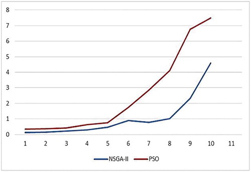
Table 6 shows that the proposed pa-PSO has a higher ability to generate better solutions than the NSGA-II algorithm. Also it produces a more diverse set of solutions than the NSGA-II algorithm. In the other words, it is more capable than the NSGA-II in exploring and finding the feasible solution region. However, the solutions of the NSGA-II are more uniform than the pa-PSO. Furthermore, Figure 4 shows the solution time for both algorithms that indicates the elapsed time of the pa-PSO is more than that of the NSGA-II algorithm.

Figure 4. Computational times of two algorithms for 10 test problems

The case study with general information shown in Table 7 is also solved with both of the algorithms. The results are shown in Table 8.

Table 7. General information for the case study problem

Indices	u	l	TC	TD	TS	TK	p	t	c	j	i	h	s
Values	3	14	4	5	2	3	41	12	21	2	2	10	2

Table 8. Objective functions values of non-dominated solutions from two algorithms

pa-PSO		NSGA-II
f1	f2	f1	f2
1174525	624633.3	1164585	792463.3
1174562.3	624662.4	1164829.8	792534.4
1174603.6	624673.5	1165388.2	792596.7
1174644.7	624690.3	1165987.6	792702
1174684.2	624719.9	1166271.7	792811.1
1174715.3	624736.9	1166647.8	792883.5
1174754.1	624763.1	1167240.6	792940.4
1174786.2	624781.9	1167775.8	793009.9
1174828	624808	1168363	793128.5
1174868.9	624826.2	1168705.4	793170.1
1174908.5	624838.6	1169107.8	793248.9
1174947.3	624856.2	1169552.6	793328.6
1174988.9	624876	-	-
1175024	624888	-	-
1175052.6	624906.7	-	-

As Table 8 indicates, the pa-PSO and the NSGA-II algorithm returned 15 and 12 non-dominated solutions, respectively.

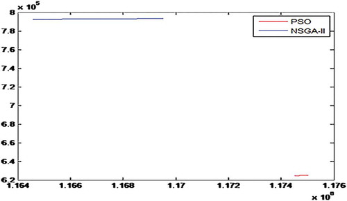
After several runs of algorithms, the metrics values in Table 9 prove that the pa-PSO performs better than the NSGA-II algorithm in finding higher quality and more diverse solutions. However, the solutions reported from the NSGA-II are more uniform. Figure 5 depicts the Pareto optimal frontier of both algorithms.

Table 9. The metric values for the proposed PSO and the NSGA-II algorithms

	Pa-PSO			NSGA-II
Diversity metric	Spacing metric	Quality metric	Diversity metric	Spacing metric	Quality metric
				metric
100	0.715	1490.3	0	0.307	1186.2

Figure 5. Pareto front of case study with two algorithms

Conclusion

Integrating production and distribution activities in supply chains and considering the environmental factors was felt to be important to be studied. Hence, in this paper a multi-objective mixed integer linear programming model was developed in a four-echelon multi-product multi-period supply chain in stone-cutting industry. The problem studied considered different types of vehicles and accounted for the CO₂ emission. The objectives of the proposed model are maximizing the profit and minimizing the CO₂ emission. First, for the purpose of validating the model, the GAMS software was utilized. Then, a multi-objective PSO based on the Pareto archive was proposed. To prove the efficiency of the proposed algorithm, a set of sample problems along with a case study was solved and the results were compared with these of NSGA-II. These results revealed that the proposed pa-PSO performs better in generating high quality and more diverse solutions. Because of the more thorough search of the feasible solution region, the pa-PSO takes a longer time than the NSGA-II algorithm. However, the NSGA-II returns more uniform solutions. For further research, other appropriate objectives such as failure minimization and service level maximization can be recommended. Also, considering more than four echelons for the supply chain- if required, applying the fuzzy goal programming approach to optimize the objectives, and solving the model with other metaheuristic algorithms are of great value.

References

- Barbarosoğlu, G., and D. Özgür. 1999. Hierarchical design of an integrated production and 2-echelon distribution system. European Journal of Operational Research 118 (3):464–84. doi:10.1016/S0377-2217(98)00317-8.
- Deb, K., A. Pratap, S. Agarwal, and T. Meyarivan. 2002. A fast and elitist multiobjective genetic algorithm: NSGA-II. IEEE Transactions on Evolutionary Computation 6 (2):182–97. doi:10.1109/4235.996017.
- Dekker, R., J. Bloemhof, and I. Mallidis. 2012. Operations research for green logistics – An overview of aspects, issues, contributions and challenges. European Journal of Operational Research 219 (3):671–79. doi:10.1016/j.ejor.2011.11.010.
- Fahimnia, B., R. Z. Farahani, R. Marian, and L. Luong. 2013. A review and critique on integrated production–distribution planning models and techniques. Journal of Manufacturing Systems 32 (1):1–19. doi:10.1016/j.jmsy.2012.07.005.
- Gholamian, N., I. Mahdavi, and R. Tavakkoli-Moghaddam. 2016. Multi-objective multi-product multi-site aggregate production planning in a supply chain under uncertainty: Fuzzy multi-objective optimisation. International Journal of Computer Integrated Manufacturing 29 (2):149–65. doi:10.1080/0951192X.2014.1002811.
- Guillén-Gosálbez, G., and I. Grossmann. 2010. A global optimization strategy for the environmentally conscious design of chemical supply chains under uncertainty in the damage assessment model. Computers & Chemical Engineering 34 (1):42–58. doi:10.1016/j.compchemeng.2009.09.003.
- Guillén-Gosálbez, G., and I. E. Grossmann. 2009. Optimal design and planning of sustainable chemical supply chains under uncertainty. AIChE Journal 55 (1):99–121. doi:10.1002/aic.11662.
- Liu, S., and L. G. Papageorgiou. 2013. Multiobjective optimisation of production, distribution and capacity planning of global supply chains in the process industry. Omega 41 (2):369–82. doi:10.1016/j.omega.2012.03.007.
- Mastrocinque, E., B. Yuce, A. Lambiase, and M. S. Packianather. 2013. A multi-objective optimisation for supply chain network using the bees algorithm. International Journal of Engineering Business Management 5:1–11.
- Mavrotas, G. 2009. Effective implementation of the ε-constraint method in multi-objective mathematical programming problems. Applied Mathematics and Computation 213 (2):455–65. doi:10.1016/j.amc.2009.03.037.
- Memari, A., A. R. A. Rahim, and R. B. Ahmad. 2015. An Integrated production-distribution planning in green supply chain: A multi-objective evolutionary approach. Procedia CIRP 26:700–05. doi:10.1016/j.procir.2015.03.006.
- Mirzapour Al-E-Hashem, S. M. J., A. Baboli, S. J. Sadjadi, and M. B. Aryanezhad. 2011. A multiobjective stochastic production-distribution planning problem in an uncertain environment considering risk and workers productivity. Mathematical Problems in Engineering 2011:1–14. doi:10.1155/2011/406398.
- Mirzapour Al-E-Hashem, S. M. J., H. Malekly, and M. B. Aryanezhad. 2011. A multi-objective robust optimization model for multi-product multi-site aggregate production planning in a supply chain under uncertainty. International Journal of Production Economics 134 (1):28–42. doi:10.1016/j.ijpe.2011.01.027.
- Moncayo-Martínez, L. A., and D. Z. Zhang. 2011. Multi-objective ant colony optimisation: A meta-heuristic approach to supply chain design. International Journal of Production Economics 131 (1):407–20. doi:10.1016/j.ijpe.2010.11.026.
- Pasandideh, S. H. R., S. T. A. Niaki, and K. Asadi. 2015a. Bi-objective optimization of a multi-product multi-period three-echelon supply chain problem under uncertain environments: NSGA-II and NRGA. Information Sciences 292:57–74. doi:10.1016/j.ins.2014.08.068.
- Pasandideh, S. H. R., S. T. A. Niaki, and K. Asadi. 2015b. Optimizing a bi-objective multi-product multi-period three echelon supply chain network with warehouse reliability. Expert Systems with Applications 42 (5):2615–23. doi:10.1016/j.eswa.2014.11.018.
- Sadrnia, A., N. Ismail, N. Zulkifli, M. Ariffin, H. Nezamabadi-Pour, and H. Mirabi. 2013. A multiobjective optimization model in automotive supply chain networks. Mathematical Problems in Engineering 2013:1–10. doi:10.1155/2013/823876.
- Sarmiento, A., and R. Nagi. 1999. A review of integrated analysis of production–distribution systems. IIE Transactions 31 (11):1061–74. doi:10.1023/A:1007623508610.
- Sarrafha, K., S. H. A. Rahmati, S. T. A. Niaki, and A. Zaretalab. 2015. A bi-objective integrated procurement, production, and distribution problem of a multi-echelon supply chain network design: A new tuned MOEA. Computers & Operations Research 54:35–51. doi:10.1016/j.cor.2014.08.010.
- Srivastava, S. K. 2007. Green supply‐chain management: A state‐of‐the‐art literature review. International Journal of Management Reviews 9 (1):53–80. doi:10.1111/j.1468-2370.2007.00202.x.
- Tavakkoli-Moghaddam, R., M. Azarkish, and A. Sadeghnejad-Barkousaraie. 2011. A new hybrid multi-objective Pareto archive PSO algorithm for a bi-objective job shop scheduling problem. Expert Systems with Applications 38 (9):10812–21. doi:10.1016/j.eswa.2011.02.050.