A Constraint Optimization–Based Sense and Response System for Interactive Business Performance Management

ABSTRACT

A Sense and Respond (SaR) system endows a Business Intelligence system with the intelligence needed to react timely to exogenous as well as endogenous events. To this end, a SaR system needs to know the Key Performance Indicators (KPIs) that must be maximized as well as their relative weights. While the first information can be easily obtained through interviews, the second one is quite hard to get. This motivates the investigation of methods and tools to address this problem.

In such a context, the main contributions of this paper are the following. First, we show how KPIs can be effectively defined using linear constraints. Second, we show how the problem of computing the actions that the SaR system proposes to the manager can be formulated as a Mixed Integer Linear Programming (MILP) problem. Third, we show how KPI weights can be computed from previous managing decisions by solving a suitable MILP problem. Fourth, we provide experimental results showing the effectiveness of the proposed approach.

1. Introduction

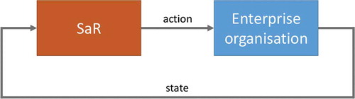
Sense and Respond (SaR) systems are among the key technological artifacts enabling the development of Business Intelligence (BI) systems. Basically, a SaR is a control system whose controlled system (plant) is an enterprise organization (see Figure 1). In such a context, sensing focuses on acquiring information about the enterprise status, while responding focuses on computing sequences of actions (typically manager actions) maximizing given Key Performance Indicators (KPIs).

Figure 1. SaR and database (DB) as a control system

1.1 Motivations

A SaR system endows a BI system with the intelligence needed to react timely to exogenous as well as endogenous events. To this end, a SaR system needs a reliable model of the enterprise organization as well as of the goals to be pursued.

Usually, a model of the enterprise organization can be derived from the enterprise DB. In fact, most SaR systems interact mainly with the enterprise DB.

The enterprise goals are much more difficult to formalize since they may involve many actors across the enterprise organization. As a result, typically we have a set of KPIs describing different requirements to be considered when automating managing decision (the SaR main goal).

While it is quite reasonable to elicit KPIs, it is much more difficult to acquire knowledge about priorities among them. Without such an information, we can only compute a partial order among the possible managing decisions. Using such a partial order, we can compute the set of all actions (i.e. managing decisions) that are Pareto optimal, i.e. cannot be improved w.r.t. all KPIs.

We note however that, in order to effectively deploy a SaR system to support BI, we need to select one action among those that are Pareto optimal. This entails computing suitable weights for the enterprise KPIs. Unfortunately, such weights are very hard to obtain since, basically, they formalize how a manager weights KPIs, and very seldom a manager is able (or willing) to state rules clearly defining priorities among KPIs.

Indeed, weighting KPIs is among the main obstacle to overcome in order to deploy SaR systems within complex organizations. This motivates the investigation of methods and tools to compute automatically KPI weights from the observation of previous manager actions. This is the main focus of the present paper.

1. 2. Contributions

Our main contributions can be summarized as follows.

First, we show how KPIs can be effectively defined using linear constraints.

Second, we show how the problem of computing reaction rules, i.e. the actions that the SaR system proposes to the manager (SaR actions), can be formulated as a constraint problem with mixed integer- and real-valued decision variables over linear constraint (Mixed Integer Linear Programming [MILP]).

Third, we show how also KPI weights can be computed from the manager decisions by solving suitable constraint (MILP) problems.

Fourth, we experimentally show that the constraint problems defined above can be efficiently solved by standard MILP solvers on real business scenarios.

1. 3. Related Work

SaR systems are at the very heart of BI systems (see, e.g. Dutta, Lee, and Yasai-Ardekani 2014; Negash and Gray 2008), and in such a context, they have been widely studied as outlined below.

The study by Haeckel and Slywotzky (1999) presents a conceptual organization for an enterprise aiming at supporting BI through a SaR system. In such a context, following a model-driven architecture (see, e.g. Huang, Kumaran, and Chung 2005; OMG Object Management Group 0000), an enterprise organization is seen as a hierarchical system consisting of four layers: (1) A strategic layer defining the enterprise objectives (see, e.g. Kaplan and Norton 1992). (2) An operational layer defining how the enterprise plans to pursue its objectives and the KPIs used to measure progress toward such objectives. (3) An executive layer defining the workflow and the information flow used to implement the operational layer. (4) An implementation layer defining the IT used to implement the executive layer. Here, we take the enterprise organization as an input and focus on the development of the SaR system itself.

The survey by Kapoor et al. (2005) presents two SaR systems: one for the IBM Microelectronics Division in Burlington Vermont and another one for the IBM Personal Computing Division in Raleigh, North Carolina. A SaR system to support supply chain management is presented in Buckley et al. (2005). The SaR design approach outlined by Kapoor et al. (2005) rests on the concepts of business component (see, e.g. Herzum and Sims 2000) to model business processes and web services (see, e.g. Gottschalk et al. 2002) for the software implementation of business components.

Nguyen, Schiefer, and Tjoa (2005) propose an event-driven SaR service architecture (SARESA) to operate BI applications. SARESA enables real-time analytics across corporate business processes, notifies the business of actionable recommendations, or automatically triggers business operations, thereby effectively closing the gap between BI systems and business processes.

Data warehousing and BI approaches are widely used as a middleware layer for state-of-the-art decision support. However, they do not provide sufficient support in dealing with real-time and closed-loop decision-making. The work by Seufert and Schiefer (2005) proposes a SaR BI architecture aiming at increasing BI value by reducing action time and interlinking business processes with decision-making.

Developments of SaR systems to support supply chain management have been investigated (e.g. Deshmukh and Mohan 2016; Hahn and Packowski 2015; Lusch, Liu, and Chen 2010; Lush 2011).

The use of SaR systems to enable the use of big data in supply chain management has been investigated by Hazen et al. (2016).

From the above, it follows that, although SaR development has been thoroughly investigated in many settings, mechanisms to endow SaR systems with machine learning methods enabling them to automatically adapt to the enterprise manager strategy, to the best of our knowledge, have not been developed so far. In this paper, we focus exactly on this point, and we do this by exploiting off-the-shelf artificial intelligence constraint-based solvers to perform the required reasoning.

Among the different modeling and solving paradigms available (see, e.g. Mancini et al. 2008; Neumaier et al. 2005), we opt for MILP, one of the most mature technologies available on the market, very popular in many industry domains (see, e.g. Caballero and Grossmann, 2014; Heilporn, De Giovanni, and Labbé 2008; Mancini et al. 2018b; Van den Bergh et al. 2013; Wang, Brandt-Pearce, and Subramaniam 2015, just to mention a few examples) including business process optimization and scheduling (see, e.g. Kyriakidis, Kopanos, and Georgiadis 2012; Sakellaropoulos and Chassiakos 2004; Vergidis, Tiwari, and Majeed 2007).

2. System Description

In this section, we describe the functional scheme of the proposed SaR system, the system components, the activity diagrams, and the business data gathering modules.

2. 1. Functional Scheme

In Figure 2, the functional scheme of the proposed SaR system is shown.

Figure 2. Functional scheme and main components of the proposed SaR system

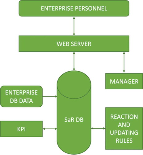
Sensing of enterprise data is realized through the enterprise DB or through web closed-form questionnaires filled by the enterprise staff. Collected data are then stored in the SaR DB through a web server, interfaced also with the enterprise manager. Data stored in the SaR DB are used to compute enterprise KPIs, as well as reaction and learning and updating rules.

The reaction rules suggest actions to the manager, who can either accept and implement them or choose other actions. The actions chosen by the manager are stored in the DB and used to update the reaction rules, if needed. The flow of the manager chosen actions reaches the enterprise organization through the enterprise DB.

2.2. System Components

Our system consists of a set of functionally dependent components (see Figure 2). The main components are the following:

• The SaR-DB component which, in addition to its own function, has also the role of communication bus among the other components.

• The Enterprise-DB component, representing all databases of the enterprise.

• The Sensor component, i.e. the software that reads data from Enterprise-DB and stores them in the SaR-DB.

• The Rules component, i.e. the software that reads KPI values from SaR-DB, stores possible corrective actions in the database, reads from SaR-DB actions executed by the manager, and updates the reaction rules. This component only needs to interface with the SaR-DB.

• The KPI component, i.e. the software that reads data from SaR-DB, computes the KPI values, and stores new KPI values in the database. Also, this component only needs to interface with the SaR-DB.

• The Web-server component, having two interfaces: the IManager interface, which allows the manager to read the action computed by the SaR from the DB and to store the action really adopted by the manager in the database; the IEnterprise interface, which allows the staff to insert enterprise data, by, e.g. filling web forms.

• The Manager component, which represents the enterprise manager. In particular, it represents the manager behavior, and it is not a software component. Indeed, it can be considered a human-in-the-loop component. The manager receives suggestions from the SaR (as actions stored in the DB), by means of the IManager interface. Then, he/she stores the action actually chosen and adopted into the DB.

• The Enterprise component stores data (collected from hard or web forms) into the SaR-DB and receives information from the SaR by means of the IEnterprise interface. The Enterprise component, which, like the Manager component, is not software, represents the enterprise behavior.

2. 3. Activity Diagrams

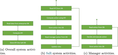
In Figure 3, the main activities of the proposed SaR are shown as UML activity diagrams, as outlined below. Figure 3(a) shows the UML activity diagram for the overall system. Figure 3(b) shows the UML activity diagram for the data reading from the enterprise DB, form reading, and KPI computation. Figure 3(c) shows the UML activity diagram for the manager. Although the manager is not a software component, he is obviously included in the learning and updating loop since his/her behavior is used by the SaR system.

Figure 3. UML activity diagrams of the proposed SaR

2. 4. Business Data Gathering

Data that flow into the DB come either from other DB of the enterprise or from web forms. Such data are collected through the subsystems (macro-blocks) described below, which correspond to specific areas of the enterprise organization. The macro-blocks below, typically occurring in most enterprises, can be considered general components.

• The Sales subsystem includes all promotional activities, oriented at contacting potential customers, such as the preparation of the economic offers to be brought to the attention of potential customers. Likewise, it must be possible to acquire the offers that suppliers submit to the company. The Sales subsystem must therefore allow the management of customer and supplier data that will then be used also by the other modules.

• The Production subsystem records all the production activities carried out in the company and organized according to the projects or the departments where they are carried out. Data collected in the Production subsystem hence allow control of the usage of company resources and enable delay tracking.

• The Administration subsystem registers the company tax accounting records.

• The Statistical subsystem provides company data analytics and forecasting.

3. Framework

In this section, we give some preliminary and background notions, and we show how to define KPIs through linear constraints.

3. 1. SaR System

A control system consists of a plant (controlled system) and a controller (controlling system). The controller reads the state of the plant and sends commands to meet given goals, in an endless loop.

In our case, the plant is the enterprise DB, and the state of the plant is given by the DB values (resources, projects, etc.).

Control actions typically define possible allocations of resources to projects and are usually decided by an expert manager, who takes into account what must be optimized (see, e.g. Mancini, Flener, and Pearson 2012 and references therein for planning approaches from relational database models).

Our goal is to design a controller that, after a training period, suggests the same control actions that an expert manager would choose.

In this context, the control system is called SaR system since it reads the state from the DB and writes the computed action back into the DB.

Formally, the plant can be modeled as a tuple P= ($\mathbf{x}$, $\mathbf{u}$, $I$, $N$), where $\mathbf{x}$ is a vector of state variables, $\mathbf{u}$ is a vector of input variables, $I$ is the set of plant initial states, and $N$ is a function computing the plant next state from the present plant state and input action. Then, the controller is a function $K$ that selects the control action $\mathbf{u}$ on the basis of plant state information $\mathbf{x}$. That is:

$\mathbf{u}(t)=K(\mathbf{x}(t-k),\mathbf{x}(t-k+1),...,\mathbf{x}(t)),$

assuming that the controller has memory horizon $k$.

Analogously to demand-response systems (see, e.g. Hayes et al. 2017; Mancini et al. 2015a, 2014b), our SaR execution consists in an endless repetition of three operations, shown in Figure 3:

1. Computation of SaR control action $\mathbf{u}$;

2. Acquisition of the control action $\mathbf{u}{ }^{\mathrm{\prime }}$ actually chosen by the manager ($\mathbf{u}$ and $\mathbf{u}{ }^{\mathrm{\prime }}$ may be different);

3. Update of KPI weights on the basis of manager control actions.

3.2. System States and Actions

Here, we outline how we encode the system state and manager actions to ease our MILP formulation. Data are taken from the DB.

A system state is an assignment to a given set of variables over integer or real domains. For example, a system state variable may define the total number of available staff members of a given seniority level operating in the enterprise or assigned to a given project.

The actions undertaken by the manager are defined by variables over integer or real domains. For example, an action may define the hiring of a given number of new staff members with a given seniority level or the reallocation of a given number of staff members to a given project.

3.3. Linear Predicates

A linear expression $L(X)$ is a linear combination of variables in $X$ with rational coefficients. A linear constraint (just constraint in the following) over $X$ is an expression of the form $L(X)\le b$, where $b$ is a rational constant. Linear predicates (just predicates in the following) are inductively defined as follows. A constraint $C(X)$ is a predicate over $X$. If $A(X)$ and $B(X)$ are predicates, then $(A(X)\wedge B(X))$ and $(A(X)\vee B(X))$ are predicates over $X$. A conjunctive predicate is a conjunction of constraints. In such a setting, a MILP problem can be seen as a pair ($J(X)$, $P(X)$) where $J(X)$ is a linear expression over decision variables $X$ (objective function) and $P(X)$ is a conjunctive predicate over $X$.

We assume any variable $x\in X$ belongs to a (real or discrete) domain $D_x$ in the form [$L_x$, $U_x$]. This means that all decision variables are bounded. With such a hypothesis, it is possible to show that any predicate can be transformed into a conjunctive predicate (e.g. see Gottlob, Greco, and Mancini 2007; Mari et al. 2010; Mari et al. 2014).

For example, in our setting (bounded decision variables), if $y$ is a fresh variable (i.e. it is not in $X$), $A(X)$, $B(X)$ are linear expressions, and $p(X)$ is a linear constraint, then expression

$y=\mathbf{i}\mathbf{f}p(X)\mathbf{t}\mathbf{h}\mathbf{e}\mathbf{n}A(X)\mathbf{e}\mathbf{l}\mathbf{s}\mathbf{e}B(X),$

is a linear predicate, which can thus be transformed into a conjunctive predicate.

Using the if-then-else construct, many functions can be expressed as linear predicates.

For example, $y=|L(X)|$ can be written as

$y=\mathbf{i}\mathbf{f}\hspace{0.17em}L(X)\le 0\hspace{0.17em}\mathbf{t}\mathbf{h}\mathbf{e}\mathbf{n}\hspace{0.17em}-L(X)\mathbf{e}\mathbf{l}\mathbf{s}\mathbf{e}\hspace{0.17em}L(X).$

Thus, the absolute value operator can be defined using conjunctive predicates.

In the following, unless otherwise stated, it is to be understood that all predicates can be transformed into conjunctive predicates. This will allow us to easily define learning rules through MILP problems.

3. 4. Key Performance Indicators

Consider the plant in. A KPI $h$ associates to a state–action pair ($\mathbf{x}$, $\mathbf{u}$) a real number $h(\mathbf{x},\mathbf{u})\in [0,1]$. That is, $h(\mathbf{x},\mathbf{u})$ defines the value of action $\mathbf{u}$ in state $\mathbf{x}$.

Note that $h(\mathbf{x},\mathbf{u})$ denotes an array consisting of $q$ KPIs, that is $h(\mathbf{x},\mathbf{u})$ = $[h_1(\mathbf{x},\mathbf{u}),\cdots ,h_q(\mathbf{x},\mathbf{u})]$. If $q\ge 2$, the array $h(\mathbf{x},\mathbf{u})$ induces a partial order (not a total order) on control actions.

Through his/her actions, an enterprise manager associates a total order to the partial order defined by the KPIs (similarly to Mancini et al. 2017; Mancini et al. 2016a; Mancini et al. 2016b). This is equivalent to associate weights expressing the relative importance of each KPI w.r.t. the others (as in, e.g. Mancini et al. 2018a).

As we aim at using MILP technology, we define KPIs as piecewise linear functions along the lines of, e.g. Mancini (2016). Note that it is always possible with any desired approximation. Hence, a KPI $h_i(\mathbf{x},\mathbf{u})$, $i=1,\dots q$ is defined through a conjunctive predicate (see Section 3.3): $H_i(\mathbf{x},\mathbf{u},\mathbf{y},z)$ such that:

$\mathrm{\exists }{y}_i{H}_i(\mathbf{x},\mathbf{u},{\mathbf{y}}_i,z_i)=1\mathrm{i}\mathrm{f}\mathrm{f}[h_i(\mathbf{x},\mathbf{u})=z_i].$

4. Computation

At system initialization, KPI weights are set to predefined values (namely: uniformly distributed values, along the lines of Mancini et al. 2014a). Then, the system enters the loop outlined in waiting for a manager request to propose a corrective action.

Upon such a request, the system computes and returns the optimal control action $u$ using the known KPI weights, as outlined in. The manager either accepts the proposed action or chooses a different action.

In the latter case, the system revises the KPI weights accordingly, as outlined in, and starts a new iteration.

Both computation tasks are performed by solving MILP problems.

4.1. Computing Optimal Actions

The SaR system chooses the next proposed actions so as to maximize a weighted combination of KPIs (as in, e.g. Mancini et al. 2015b; Tronci et al. 2014) using the current values for the weights. In particular, the objective function $J$ to maximize is of the form:

$J=\sum _{i=1}^q{w}_i{h}_i(\mathbf{x},\mathbf{u})=\mathbf{w}\cdot h(\mathbf{x},\mathbf{u}),$

where $\mathbf{w}$ = [$w_1,\dots ,w_q$], with $w_i\ge 0$ ($i=1,\dots ,q$) and ${\sum }_{i=1}^q{w}_i=1$.

By representing KPIs as convex predicates as outlined in, our MILP problem is as follows:

$\begin{array}{rl}& \mathrm{m}\mathrm{a}\mathrm{x}\mathrm{i}\mathrm{m}\mathrm{i}\mathrm{z}\mathrm{e}\sum _{i=1}^q{w}_i{z}_i\\ & \mathrm{s}\mathrm{u}\mathrm{b}\mathrm{j}\mathrm{e}\mathrm{c}\mathrm{t}\mathrm{t}\mathrm{o}{H}_i(\mathbf{x},\mathbf{u},{\mathbf{y}}_i,z_i)i=1,\dots ,q^{.}\end{array}$

The decision variables in the above MILP problem are $\mathbf{u}$, ${\mathbf{y}}_1,\dots ,{\mathbf{y}}_q$, $z_1,\dots z_q$. In fact, note that values for state variables $x$ are known (as they are retrieved from the DB), and values for KPI weights $\mathbf{w}$ are those available from the previous step.

An optimal solution to the above MILP problem also gives values for the optimal control actions $\mathbf{u}$ to be proposed to the manager. Note that such actions are optimal under current evidence, as they maximize the resulting value of the linear combination of KPIs with the known weights.

4.2. Revising KPI Weights

In case the control actions proposed by the SaR are rejected, the system revises KPI weights ($\mathbf{w}$) on the basis of the control actions actually chosen by the manager.

At each iteration $t$ of the system execution loop, let:

• $\mathbf{x}(t)$ be the values of the system state variables at iteration $t$;

• $\mathbf{u}(t)$ be the values of the optimal control actions computed by the system at iteration $t$;

•${\mathbf{u}}^{\prime }(t)$ be the values of the actions actually chosen by the manager at iteration $t$, after having rejected $\mathbf{u}(t)$;

• $\mathbf{w}(t)$ be the values of the KPI weights at iteration $t$;

• ${\mathbf{w}}^{\prime }(t)$ be the values of the KPI weights chosen by the manager at iteration $t$.

Then, on the basis of such values, the system computes values for $\mathbf{w}(t+1)$, i.e. new KPI weights to be used from iteration $t+1$.

Optimal values for $\mathbf{w}(t+1)$ are again computed using a MILP solver. In particular, a sliding window of length $k$ is defined starting from iteration $t$, such that $t-k+1\ge 0$. Values for $\mathbf{w}(t+1)$, depend on $\mathbf{x}(\tau )$, $\mathbf{u}(\tau )$, ${\mathbf{u}}^{\prime }(\tau )$, for $\tau \in [t-k+1,t]=\{t-k+1,\dots ,t\}$.

Also, $\mathbf{w}(t+1)$ must satisfy the following requirements:

• For each past iteration $\tau$ $\in$ $[t-k+1,t]$, the actions actually chosen by the manager in $\tau$ ($\mathbf{u}{ }^{\mathrm{\prime }}(\tau )$) should be preferable to those that the system suggested ($\mathbf{u}(\tau )$). In other words, the new weights should be consistent with the knowledge accumulated by the system during the sliding window. Formally, for each $\tau$ $\in$ $[t-k+1,t]$ must be

$\mathbf{w}(t+1)(h(\mathbf{x}(\tau ),{\mathbf{u}}^{\prime }(\tau ))-h(\mathbf{x}(\tau ),\mathbf{u}(\tau )))\ge \delta ,$

where the value of $\delta$ must be small but not null (for example, $\delta \ge 0.001$).

• Values for $\mathbf{w}(t+1)$ are not very different from those of $\mathit{w}(t)$. This constraint is needed to avoid oscillations of KPI weights which could prevent convergence. This means minimizing the quantity:

$\begin{array}{rl}& W(t)=\sum _{\tau =t-k+1}^t||\mathbf{w}(t+1)-\mathbf{w}(\tau )||=\\ & =\sum _{\tau =t-k+1}^t\sum _{i=1}^q|w_i(t+1)-w_i(\tau )|.\end{array}$

Such requirements are defined in terms of linear constraints in the MILP problem, using additional parameters (e.g. for the latter constraint) which can be configured by the user. The solution of the MILP problem provides the new array for KPI weights $\mathbf{w}(t+1)$, using the decision variables $\mathbf{w}(t+1)$, $\delta$ and $y_{\tau ,i}$, and $W(t)$ is computed through the conjunctive predicate $\mathrm{A}bsVal$. The above considerations lead to the following optimization problem.

$\begin{array}{cc}min& \delta +\sum _{\tau =t-k+1}^t\sum _{i=1}^q\hspace{0.17em}{y}_{\tau ,i}\\ \hspace{0.17em}& \hspace{0.17em}\end{array},$

subject to:

$\begin{array}{ccc}\mathbf{w}(t+1)(h(\mathbf{x}(\tau ),{\mathbf{u}}^{\prime }(\tau ))-h(\mathbf{x}(\tau ),\mathbf{u}(\tau )))-\delta & \ge & 0\tau \in [t-k+1,t]\\ \delta & \ge & 0.001\\ \hspace{0.17em}& \hspace{0.17em}& \hspace{0.17em}\\ \mathrm{A}\mathrm{b}\mathrm{s}\mathrm{V}\mathrm{a}\mathrm{l}(q,y_{\tau ,i},w_i(t+1),w_i(\tau ))& \hspace{0.17em}& \tau \in [t-k+1,t],i\in [1,q]\end{array}$

5. Experimental Evaluation

This section presents an experimental evaluation of our SaR aiming at assessing the efficacy of our approach.

5.1. Implementation

We have implemented our SaR using freely available relational DB connectivity libraries and the PostgreSQL relational DBMS. Our implementation relies on the well-known open-source GLPK MILP solver (GLPK 1989) to compute optimal control actions and to revise KPI weights when needed.

5.2. Case Study

We deployed our SaR for evaluation at a medium-sized multimedia enterprise, our partner in a national project which funded this research.

The enterprise runs multiple simultaneous multimedia projects (consisting of sequences of tasks) for its customer portfolio. The advancement of such projects is strictly monitored, and staff members of different seniority levels (and costs) are frequently reassigned to tasks lagging behind their schedule, in order to meet intermediate and final deadlines.

Data about active projects, tasks, available staff members, possible corrective actions, etc., are stored in a relational DB. When comes to MILP encoding, data about projects, tasks, and staff members are used to assign values to the following variables. Depending on the MILP problem considered (the one in or the one in, some of such variables are decision variables, while the others act as constants.

5.3. System State

The system state is encoded by a set of variables taking values within proper integer ranges. Some variables have values constant throughout the system evolution.

A list follows (we show variable names only if used in the scenarios of the following sections): overall number of junior ($N_j$) and senior ($N_s$) staff members (totaling $N_{tot}$ = $N_j+N_s$); number of junior ($N_j^x$) and senior ($N_s^x$) staff members currently working on task $x$; overall number of working days for junior ($T_j$) and senior ($T_s$) staff members; average number of working days for junior ($G_j\mathrm{\_}avg$) and senior ($G_s\mathrm{\_}avg$) staff; overall number of working days ($G_{tot}$); average number of working days for junior/senior staff for each customer; total number of working days for each customer; number of customers having at least a junior/senior staff member; total number of customers; average and per-project salary for junior and senior staff members; and total cost for each project.

5.4. Control Actions

Possible control actions, again encoded as integer-valued variables, envision increase/reduction of the overall number of junior ($a_j$) or senior ($a_s$) staff members (where negative values denote reductions) or of staff members having a given seniority level and assigned to a given task ($a_j^x$ and $a_s^x$, respectively, where $x$ denotes a task) or customer; increase/reduction of the number of working days for junior ($t_j$) and senior ($t_s$) staff members.

5.5. Evaluation Goals and Methodology

In the following, we show the effectiveness of our system on some of the scenarios provided by the managers of the enterprise participating in our project.

Such scenarios consist of initial values for the system state variables as well as a strategy followed by the manager to choose optimal actions. Such a strategy has been conveniently transformed back into KPI weights $\mathbf{w}{ }^{\mathrm{\prime }}(t)$which are constant over time and unknown to the system.

Hence, the goal of our evaluation activity is to show how fast the KPI weights used and revised by the system converge to those actually defining the real strategy of the manager.

We note that, given the small size of the MILP problems generated in these realistic scenarios, computation times are always negligible and compatible with an interactive use of the platform. To this end, in the following, we do not comment on such computation times.

5.6. Evaluation Scenario with 2 KPIs

The first scenario defines only two KPIs, namely, juniority and seniority rates of staff members, computed, respectively, as:

$z_0=\frac{N_j+a_j}{N_{tot}},z_1=\frac{N_s+a_s}{N_{tot}}.$

By selecting such KPIs, the SaR constraint problem encoder also adds the following additional constraints to the generated MILP:

• $N_j+a_j+N_s+a_s\le N_{tot}$,

• $N_j+a_j\ge 0$, and

• $N_s+a_s\ge 0$.

Our scenario envisions the following initial values for state variables: $N_j=N_s=50$, $N_{tot}=100$, and a manager actual strategy for choosing control actions defined by the following KPI weights: $\mathbf{w}{ }^{\mathrm{\prime }}=[0.1,0.9]$ (which are unknown to the system).

Iteration 1 – The system starts its operations by setting: $\mathbf{w}(1)=[0.5,0.5]$ and proposes the following control action ($\mathbf{u}$): $a_j=+50$, $a_s=-50$.

This action implies the following new values for the KPIs: $z_0=1.0$, $z_1=0.0$.

Conversely, from $\mathbf{w}{ }^{\mathrm{\prime }}$, we can compute the action ($\mathbf{u}{ }^{\mathrm{\prime }}$) that the manager would have actually chosen, i.e. $a_j=-50$, $a_s=+50$ (which would have led to the following KPI values: $z_0=0.0$, $z_1=1.0$).

Since the action chosen by the manager is different from that computed by the system, KPI weights must be revised. After solving the MILP in, the new values for KPI weights are $\mathbf{w}(2)=[0.4995,0.5005]$.

Iteration 2 – After having updated the state according to the manager chosen action, the new state is $N_j=0$, $N_s=100$, $N_{tot}=100$.

The system, by solving the MILP of, proposes the following control action $\mathbf{u}(2)$: $a_j=0$, $a_s=0$ (i.e. do nothing), which is equal to the optimal action that is computed from $\mathbf{w}{ }^{\mathrm{\prime }}$.

Hence, in just two iterations, the revised KPI weights allow the system to converge to the action decided by the manager. This is summarized in Table 1.

Table 1. Scenario with two KPIs

-	Hidden manager weights $\mathbf{w}{ }^{\mathrm{\prime }}$	[0.1,0.9]
1	State	$N_j=N_s=50$, $N_{tot}=100$
	Manager actions $\mathbf{u}{ }^{\mathrm{\prime }}$(1)	$a_j=-50$, $a_s=+50$
	Manager KPI$\prime$	$z_0=0.0$, $z_1=1.0$
	Computed weights $\mathbf{w}$(1)	[0.5, 0.5]
	Computed actions $\mathbf{u}$(1)	$a_j=+50$, $a_s=-50$
	Computed KPI	$z_0=1.0$, $z_1=0.0$
2	State	$N_j=0$, $N_s=100$, $N_{tot}=100$
	Manager actions $\mathbf{u}{ }^{\mathrm{\prime }}$(2)	$a_j=0$, $a_s=0$
	Manager KPI$\prime$	$z_0=0.0$, $z_1=1.0$
	Computed weights $\mathbf{w}$(2)	[0.4995, 0.5005]
	Computed actions $\mathbf{u}$(2)	$a_j=0$, $a_s=0$
	Computed KPI	$z_0=0.0$, $z_1=1.0$

5.7. Evaluation Scenario with 4 KPIs

The next test has been executed adding two KPIs to the KPIs $z_0$ and $z_1$ already considered in the previous case (for two KPIs): junior and senior working days per customer, computed, respectively, as:

$z_2=\frac{G_j\mathrm{\_}avg\cdot (N_j+a_j)}{G_{tot}},z_3=\frac{G_s\mathrm{\_}avg\cdot (N_s+a_s)}{G_{tot}}.$

As for the previous case, the considered additional constraints are:

• $N_j+a_j+N_s+a_s\le N_{tot}$,

• $N_j+a_j\ge 0$, and

• $N_s+a_s\ge 0$.

Our scenario envisions the following initial values for state variables: $N_j=N_s=50$, $N_{tot}=100$, and a manager actual strategy for choosing control actions defined by the following KPI weights unknown to the system: $\mathbf{w}{ }^{\mathrm{\prime }}=[0.1,0.7,0.1,0.1]$.

The system starts (Iteration 1) its operations by setting: $\mathbf{w}(1)=[0.25,0.25,$ $0.25,$ $0.25]$ and proposes the following control action ($u$): $a_j=-35$, $a_s=-28$.

This action implies the following new values for the KPIs: $z_0=0.15$, $z_1=0.22$, $z_2=1.0$, $z_3=1.0$.

In this case, as the action $\mathbf{u}{ }^{\mathrm{\prime }}$ that the manager would have actually chosen using the real weights $\mathbf{w}{ }^{\mathrm{\prime }}$ is the same, the manager follows the system's proposed action; hence, we do not compute new weights. In other words, if the manager actions and the system computed actions are the same, the algorithm stops, even if the weights are not the same. This is because we can check not only equality between weights but also equality between actions. Indeed, running the updating algorithm again would not produce any update on the computed weights since manager and computed actions are the same.

This is summarized in Table 2.

Table 2. Scenario with four KPIs, where the system obtains the same actions decided by the manager

-	Hidden manager weights $\mathbf{w}{ }^{\mathrm{\prime }}$	[0.1,0.7, 0.1, 0.1]
1	State	$N_j=N_s=50$, $N_{tot}=100$
	Manager actions $\mathbf{u}{ }^{\mathrm{\prime }}$(1)	$a_j=-35$, $a_s=-28$
	Manager KPI$\prime$	$z_0=0.15$, $z_1=0.22$, $z_2=1.0$, $z_2=1.0$
	Computed weights $\mathbf{w}$(1)	[0.25, 0.25, 0.25, 0.25]
	Computed actions $\mathbf{u}$(1)	Same as manager
	Computed KPI	Same as manager

We observed that also changing the manager weights, the action decided by the manager and the action computed by the system are the same and remain unchanged.

We obtained different actions (manager and system) only using the following manager weights: $\mathbf{w}{ }^{\mathrm{\prime }}=[1.0,0.0,0.0,0.0]$, that is adopting only one weight equal to 1 and setting all other weights to 0. This way, we obtained the following results (remaining values are unchanged):

• Action computed by the system: $a_j=-35$, $a_s=-28$;

• KPIs computed by the system: $z_0=0.15$, $z_1=0.22$, $z_2=1.0$, $z_3=1.0$;

• Action decided by the manager: $a_j=-35$, $a_s=-50$;

• KPIs computed by the manager: $z_0=0.15$, $z_1=0.0$, $z_2=1.0$, $z_3=0.0$.

In this case, the computation of new weights is not necessary. In fact, we can notice that the action decided by the manager causes the generation of KPI values lower than those obtained using the actions computed by the SaR system. That is, the manager solution is Pareto dominated by the SaR system solution. Namely, the array of manager KPIs is component-wise less than or equal to the array of KPIs computed using the SaR system actions. As a result, the MILP that updates KPI weights is infeasible and thus new weights are not computed, and the algorithm stops. This is summarized in Table 3.

Table 3. Scenario with four KPIs, where the manager solution is Pareto dominated by the SaR system solution

-	Hidden $\mathbf{w}{ }^{\mathrm{\prime }}$	[1.0, 0.0, 0.0, 0.0]
1	State	$N_j=N_s=50$, $N_{tot}=100$
	Manager actions $\mathbf{u}{ }^{\mathrm{\prime }}$(1)	$a_j=-35$, $a_s=-50$
	Manager KPI$\prime$	$z_0=0.15$, $z_1=0.0$, $z_2=1.0$, $z_3=0.0$
	Computed weights $\mathbf{w}$(1)	[0.25, 0.25, 0.25, 0.25]
	Computed actions $\mathbf{u}$(1)	$a_j=-35$, $a_s=-28$
	Computed KPI	$z_0=0.15$, $z_1=0.22$, $z_{1}2=1.0$, $z_3=1.0$

5.8. Evaluation Scenario with 29 KPIs

A more extensive test was done by storing a set of 29 KPIs in the database, including the 4 KPIs considered for the evaluation scenario in. This set includes all the KPIs described in. Consequently, all the additional constraints that are obtained when using this set of KPIs are considered.

For this evaluation scenario, we considered two tasks $x1$ and $x2$, giving eight state variables ($N_j$, $N_s$, $N_j^{x1}$, $N_j^{x2}$, $N_s^{x1}$, $N_s^{x2}$, $T_j$, and $T_s$) and eight action variables ($a_j$, $a_s$, $a_j^{x1}$, $a_j^{x2}$, $a_s^{x1}$, $a_s^{x2}$, $t_j$, and $t_s$).

The execution of the algorithm is summarized in Table 4, where the weights adopted by the manager are listed in the first row, and the initial state values, the computed system weights, the manager actions, and the manager KPI$\prime$s, as well as the computed actions and the computed KPIs, are shown.

Table 4. Scenario with 29 KPIs

-	Hidden manager weights $\mathbf{w}{ }^{\mathrm{\prime }}$	[0.1, 0.2, 0.03, 0.03, 0.03, 0.03, 0.03, 0.03, 0.03, 0.03, 0.03, 0.03, 0.03, 0.03, 0.03, 0.03, 0.03, 0.03, 0.03, 0.03, 0.03, 0.03, 0.03, 0.03, 0.01, 0.01, 0.01, 0.005, 0.005]
1	State	$N_j=50$, $N_s=50$, $N_j^{x1}=20$, $N_j^{x2}=30$, $N_s^{x1}=10$, $N_s^{x2}=10$, $T_j=22$, $T_s=15$
	Manager actions $\mathbf{u}{ }^{\mathrm{\prime }}$(1)	$a_j=-50$, $a_s=-50$, $a_j^{x1}=-20$, $a_j^{x2}=-30$, $a_s^{x1}=-10$, $a_s^{x2}=-10$, $t_j=22$, $t_s=22$
	Manager KPI$\prime$	$z_0=0$, $z_1=0$, $z_2=0$, $z_3=0$, $z_4=0$, $z_5=0$, $z_6=0$, $z_7=0$, $z_8=1$, $z_9=0.5$, $z_{10}=0$, $z_{11}=0$, $z_{12}=0$, $z_{13}=0$, $z_{14}=0$, $z_{15}=0.76$, $z_{16}=0.78$, $z_{17}=0$, $z_{18}=0$, $z_{19}=0$, $z_{20}=0$, $z_{21}=1$, $z_{22}=1$, $z_{23}=0.22$, $z_{24}=0.44$, $z_{25}=0.11$, $z_{26}=0.07$, $z_{27}=0$, $z_{28}=0$
	Computed weights $\mathbf{w}$(1)	$\frac{1}{N_{KPI}}=\frac{1}{29}=0.034$
	Computed actions $\mathbf{u}$(1)	Same as manager
	Computed KPI	Same as manager

Also, in this case, the system converges to the action decided by the manager during the first iteration.

The observations made in the case of four KPIs are valid even when many more KPIs are taken into account, as in this case. That is, when the manager actions and the system computed actions are the same, the algorithm stops even if the weights are not the same.

6. Conclusions

One of the main obstacles to overcome in order to deploy advanced SaR systems to support BI systems is the computation of the relative weights of the KPIs defining SaR goals.

In such a context, we provided the following contributions. First, methods to define KPIs using linear constraints. Second, methods to compute reaction rules using a MILP solver. Third, methods to compute KPI weights from previous managing decisions using a MILP solver. Finally, we implemented our algorithms and presented experimental results showing the effectiveness of our proposed approach.

Acknowledgments

This research has been partially supported by the MIUR grant Excellence Departments 2018–2022 to the Computer Science Department of Sapienza University of Rome and the FP7 projects SmartHG (317761) and PAEON (600773).

Additional information

Funding

This work was supported by the EC FP7-ICT Information and Communication Technologies [317761], SmartHG (Energy Demand Aware Open Services for Smart Grid Intelligent Automation  -https://cordis.europa.eu/project/id/317761) and; EC FP7-ICT Information and Communication Technologies [600773], PAEON (Model Driven Computation of Treatments for Infertility Related Endocrinological Diseases - https://cordis.europa.eu/project/id/600773).

References

- Buckley S., Ettl M., Lin G., Wang KY.(2005) Sense and Respond Business Performance Management. In: An C., Fromm H. (eds) Supply Chain Management on Demand. Springer, Berlin, Heidelberg. https://doi.org/10.1007/3-540-27354-9_12
- Caballero, J. A., and I. E. Grossmann. 2014. Optimal synthesis of thermally coupled distillation sequences using a novel MILP approach. Computers & Chemical Engineering 61:118–35. doi:10.1016/j.compchemeng.2013.10.015.
- Deshmukh, A. K., and A. Mohan. March 2016. Demand chain management: The marketing and supply chain interface redefined. IUP Journal of Supply Chain Management 13:20–36.
- Dutta, A., H. Lee, and M. Yasai-Ardekani. 2014. Digital systems and competitive responsiveness: The dynamics of it business value. Information & Management 51 (6):762–73. doi:10.1016/j.im.2014.05.005.
- GLPK. 1989. The GLPK MILP Solver – GNU Project. http://www.gnu.org/software/glpk
- Gottlob, G., G. Greco, and T. Mancini. Conditional constraint satisfaction: Logical foundations and complexity. In Proceedings of 20th International Joint Conference on Artificial Intelligence (IJCAI 2007), Hyderabad, India, 88–93, 2007.
- Gottschalk, K., S. Graham, H. Kreger, and J. Snell. 2002. Introduction to web services architecture. IBM Systems Journal 41:170–-177. doi:10.1147/sj.412.0170.
- Haeckel, S., and A. J. Slywotzky. 1999. Adaptive enterprise: Creating and leading sense-and-respond organizations. Boston, Massachusetts: Harvard Business School Press.
- Hahn, G. J., and J. Packowski. 2015. A perspective on applications of in-memory analytics in supply chain management. Decision Support Systems 76 ( Analyzing the Impacts of Advanced Information Technologies on Business Operations):45–52. doi:10.1016/j.dss.2015.01.003.
- Hayes, B. P., I. Melatti, T. Mancini, M. Prodanovic, and E. Tronci. 2017. Residential demand management using individualised demand aware price policies. IEEE Transactions on Smart Grid 8:3. doi:10.1109/TSG.2016.2596790.
- Hazen, B. T., J. B. Skipper, J. D. Ezell, and C. A. Boone. November 2016. Big data and predictive analytics for supply chain sustainability: A theory-driven research agenda. Computers & Industrial Engineering 101 (C):592–98. doi:10.1016/j.cie.2016.06.030.
- Heilporn, G., L. De Giovanni, and M. Labbé. 2008. Optimization models for the single delay management problem in public transportation. European Journal of Operational Research 189 (3):762–74. doi:10.1016/j.ejor.2006.10.065.
- Herzum, P., and O. Sims. 2000. Business components factory: A comprehensive overview of component-based development for the enterprise. 1st ed. New York, NY, USA: John Wiley & Sons, Inc..
- Huang, Y., S. Kumaran, and J.-Y. Chung. 2005. A model-driven framework for enterprise service management. Information Systems and e-Business Management 3 (2):201–17. doi:10.1007/s10257-005-0056-8.
- Kaplan, R. S., and D. P. Norton. 1992. The balanced scorecard-measures that drive performance. Harvard Business Review 70 (1):71–9. PMID: 10119714.
- Kapoor, S., K. Bhattacharya, S. Buckley, P. Chowdhary, M. Ettl, K. Katircioglu, E. Mauch, and L. Phillips. 2005. A technical framework for sense-and-respond business management. IBM Systems Journal 44:5–24. doi:10.1147/sj.441.0005.
- Kyriakidis, T. S., G. M. Kopanos, and M. C. Georgiadis. 2012. MILP formulations for single-and multi-mode resource-constrained project scheduling problems. Computers & Chemical Engineering 36:369–85. doi:10.1016/j.compchemeng.2011.06.007.
- Lusch, R. F., Y. Liu, and Y. Chen. 2010. The phase transition of markets and organizations: The new intelligence and entrepreneurial frontier. IEEE Intelligent Systems 25 (1):71–75.
- Lush, R. F. Jan 2011. Reframing supply chain management: A service-dominant logic perspective. Journal of Supply Chain Management 47 (1):14–18. doi:10.1111/j.1745-493X.2010.03211.x.
- Mancini, T. 2016. Now or Never: Negotiating efficiently with unknown or untrusted counterparts. Fundamenta Informaticae 149 (1–2):61–100. doi:10.3233/FI-2016-1443.
- Mancini, T., E. Tronci, I. Salvo, F. Mari, A. Massini, and I. Melatti. Computing biological model parameters by parallel statistical model checking. In Proceedings of 3rd International Conference on Bioinformatics and Biomedical Engineering (IWBBIO 2015), volume 9044 of Lecture Notes in Computer Science, 542–54. Granada, Spain: Springer, 2015b.
- Mancini, T., F. Mari, A. Massini, I. Melatti, and E. Tronci. Anytime system level verification via random exhaustive hardware in the loop simulation. In Proceedings of 17th Euromicro Conference on Digital System Design (DSD 2014), Verona, Italy, 236–45. IEEE, 2014a.
- Mancini, T., F. Mari, A. Massini, I. Melatti, and E. Tronci. 2016a. Anytime system level verification via parallel random exhaustive hardware in the loop simulation. Microprocessors and Microsystems 41:12–28. doi:10.1016/j.micpro.2015.10.010.
- Mancini, T., F. Mari, A. Massini, I. Melatti, and E. Tronci. 2016b. SyLVaaS: System level formal verification as a service. Fundamenta Informaticae 1–2:101–32. doi:10.3233/FI-2016-1444.
- Mancini, T., F. Mari, A. Massini, I. Melatti, I. Salvo, and E. Tronci. 2017. On minimising the maximum expected verification time. Information Processing Letters 122:8–16. doi:10.1016/j.ipl.2017.02.001.
- Mancini, T., F. Mari, A. Massini, I. Melatti, I. Salvo, S. Sinisi, E. Tronci, R. Ehrig, S. Röblitz, and B. Leeners. Computing personalised treatments through in silico clinical trials. A case study on downregulation in assisted reproduction. In Proceedings of 25th RCRA International Workshop on Experimental Evaluation of Algorithms for Solving Problems with Combinatorial Explosion (RCRA 2018), volume 2271 of CEUR Workshop Proceedings. Oxford, UK: CEUR.org, 2018a.
- Mancini, T., F. Mari, I. Melatti, I. Salvo, and E. Tronci. An efficient algorithm for network vulnerability analysis under malicious attacks. In Proceedings of The 24th International Symposium on Methodologies for Intelligent Systems (ISMIS 2018). Limassol, Cyprus: Springer, 2018b.
- Mancini, T., F. Mari, I. Melatti, I. Salvo, E. Tronci, J. Gruber, B. Hayes, M. Prodanovic, and L. Elmegaard. Demand-aware price policy synthesis and verification services for smart grids. In Proceedings of 2014 IEEE International Conference on Smart Grid Communications (SmartGridComm 2014), 794–99. Venice, Italy: IEEE, 2014b.
- Mancini, T., F. Mari, I. Melatti, I. Salvo, E. Tronci, J. K. Gruber, B. Hayes, M. Prodanovic, and L. Elmegaard. User flexibility aware price policy synthesis for smart grids. In Proceedings of 18th Euromicro Conference on Digital System Design (DSD 2015), 478–85. Madeira, Portugal: IEEE, 2015a.
- Mancini, T., M. Cadoli, D. Micaletto, and F. Patrizi. 2008. Evaluating ASP and commercial solvers on the CSPLib. Constraints 13 (4):407–36. doi:10.1007/s10601-007-9028-6.
- Mancini, T., P. Flener, and J. Pearson. Combinatorial problem solving over relational databases: View synthesis through constraint-based local search. In Proceedings of ACM Symposium on Applied Computing (SAC 2012), 80–87. Trento, Italy: ACM, 2012.
- Mari, F., I. Melatti, I. Salvo, and E. Tronci. Synthesis of quantized feedback control software for discrete time linear hybrid systems. In Proceedings of 22nd International Conference on Computer Aided Verification (CAV 2010), volume 6174 of Lecture Notes in Computer Science, 180–95. Edinburgh, UK: Springer, 2010.
- Mari, F., I. Melatti, I. Salvo, and E. Tronci. 2014. Model based synthesis of control software from system level formal specifications. ACM Transactions on Software Engineering and Methodology 23 (1):1–42. doi:10.1145/2559934.
- Negash, S., and P. Gray. 2008. Business intelligence. In Handbook on decision support systems 2. International handbooks information system, 175–193 Berlin, Heidelberg: Springer. https://doi.org/10.1007/978-3-540-48716-6_9
- Neumaier, A., O. Shcherbina, W. Huyer, and T. Vinkó. 2005. A comparison of complete global optimization solvers. Mathematical Programming 103 (2):335–56. doi:10.1007/s10107-005-0585-4.
- Nguyen, T. M., J. Schiefer, and A. M. Tjoa. Sense & response service architecture (SARESA): An approach towards a real-time business intelligence solution and its use for a fraud detection application. In Proceedings of the 8th ACM International Workshop on Data Warehousing and OLAP, DOLAP ‘05, 77–86, New York, NY, USA, 2005. ACM.
- OMG Object Management Group. 0000. Model driven architecture. http://www.omg.org/mda/.
- Sakellaropoulos, S., and A. P. Chassiakos. 2004. Project time–cost analysis under generalised precedence relations. Advances in Engineering Software 35 (10–11):715–24. doi:10.1016/j.advengsoft.2004.03.017.
- Seufert, A., and J. Schiefer. Enhanced business intelligence – Supporting business processes with real-time business analytics. In DEXA Workshops, 919–25. Copenhagen, Denmark: IEEE Computer Society, 2005.
- Tronci, E., T. Mancini, I. Salvo, S. Sinisi, F. Mari, I. Melatti, A. Massini, F. Davi’, T. Dierkes, R. Ehrig, et al. Patient-specific models from inter-patient biological models and clinical records. In Proceedings of 14th International Conference on Formal Methods in Computer-Aided Design (FMCAD 2014), 207–14. Lausanne, Switzerland:IEEE, 2014.
- Van den Bergh, J., P. De Bruecker, J. Beliën, L. De Boeck, and E. Demeulemeester. 2013. A three-stage approach for aircraft line maintenance personnel rostering using MIP, discrete event simulation and DEA. Expert Systems with Applications 40 (7):2659–68. doi:10.1016/j.eswa.2012.11.009.
- Vergidis, K., A. Tiwari, and B. Majeed. 2007. Business process analysis and optimization: Beyond reengineering. IEEE Transactions on Systems, Man, and Cybernetics, Part C (Applications and Reviews) 38 (1):69–82. doi:10.1109/TSMCC.2007.905812.
- Wang, X., M. Brandt-Pearce, and S. Subramaniam. 2015. Impact of wavelength and modulation conversion on translucent elastic optical networks using MILP. Journal of Optical Communications and Networking 7 (7):644–55. doi:10.1364/JOCN.7.000644.