Quadrotor Attitude Dynamics Identification Based on Nonlinear Autoregressive Neural Network with Exogenous Inputs

ABSTRACT

In the case of quadrotors, system identification is a challenging task because quadrotors are inherently unstable exhibit nonlinear behavior and significant coupling. In addition to this, quadrotors’ behavior is greatly influenced by characteristics and coefficients, which are very hard to measure directly or determine analytically. However, all the difficulties listed above are known to be successfully overcome by the use of artificial intelligence. In this paper, two system identification techniques were applied and compared to model quadrotor attitude dynamics. These techniques are Nonlinear Autoregressive Network with Exogenous Inputs (NARX) and continuous-time transfer function.

Introduction

The last decade has seen a great increase in the use of machine learning techniques. They have been successfully used to solve a huge range of engineering and scientific problems. Over the past couple of years, it was shown that artificial neural networks can successfully control systems as complicated as pneumatic artificial muscles (Nguyen, Cao, and Huy Anh 2017). Machine learning managed to improve post-processing of sensor array readings for speed measurements of an underwater vehicle (Wilmer et al. 2020). Jaradat and Mamoun (2016) used neural networks for sensor fusion in their INS/GPS navigation system. At the same time, Gharajeh and Jond (2020) relied on ANFIS for global positioning in their autonomous mobile robot. In their work, Sezginer and Kasnakoglu (2019) have used NARX artificial neural networks to control an aircraft during take-off and landing, which are known to be the most critical control problem in aircraft navigation. Altan, Aslan, and Hacioglu (2018) showed that NARX can be used to achieve a better path tracking performance for a hexarotor UAV. A lot of these advancements relate in one way or another to UAVs, their control and navigation. This should not come as a surprise given the rate of growth of this field. Days when launching a drone was exclusively an academic activity are long gone. Today their applications are extremely diverse and include things like delivering goods, vessel emission monitoring (Yuan et al. 2020) and volcano observation (Granados-Bolanos, Quesada-Roman, and Alvarado 2020). Such a wide range of applications presents engineers with ever-increasing demand for more complex control algorithms. However, designing and testing a control algorithm for a UAV is not a trivial task. The most obvious problem is that a failure of a controller to stabilize the system will immediately result in a UAV crashing. This results in damage or complete destruction of expensive equipment and slows down the design process. Such challenges are usually overcome by use of computer modeling techniques because a model can run a lot faster than a real experiment and it cannot damage itself. Due to these remarkable advantages, there is always a demand for new, better methods to model dynamic systems in general and aerial vehicles in particular. There are several publications related to this topic. Xiaodong et al. (2014) present a comprehensive survey of different approaches to quadrotor modeling, including white, gray and black box models. In his master thesis, Bresciani (2008) shows the process of designing and building a quadrotor. The author relies on first principles and measurements of the required parameters to model the system and design a controller. To reinforce this approach many researchers have shown how rotorcraft parameters can be measured (Bergamasco and Lovera 2014; Elsamanty et al. 2013). However, most of the literature focuses on gray-box approach (Kim, Kang, and Park 2009; Pounds, Mahony, and Corke 2006, 2010). In these cases, authors derive equations of the system from first principles but use data-driven techniques to estimate parameters of the system. In the end, they obtain three continuous transfer functions to represent the system. In his work Qianying (2014) used linear transfer functions in combination with a Kalman filter to identify system parameters. However, most authors point out that modeling an aerial vehicle is made hard by its nonlinear behavior and significant amount of coupling present. At the same time, it had been shown that machine learning techniques are very efficient at capturing such dynamics. Parvaresh and Moosavian (2019) have successfully used NARX to model a continuum robotic arm. Neural networks were used to create a black box model of buckling-restrained braces (Assaleh, AlHamaydeh, and Choudhary 2015). Bayat, Pishkenari, and Salarieh (2019) designed an observer for a nano-positioning system based on ANFIS ANN, while Hosovsky et al. (2016) have to use NARX to model a two-link robot with pneumatic muscles. In their work, Kislitsyna and Malykhina (2017) propose a method for determining the motion parameters of the module de-orbiting upon the lunar surface, which is based on a recursive neural network. Authors of this paper propose a method of modeling quadrotor UAVs using NARX artificial neural networks and presents experimental results obtained.

This paper is structured as follows: Section 1 provides an introduction and an outline of the paper. Section 2 provides the necessary background knowledge. Section 3 describes the system layout and experimental setup. Section 4 provides an overview of the methods used to obtain the models. At last, section 5 presents experimental results.

Quadrotor Reference Frame and Control

Reference Frame

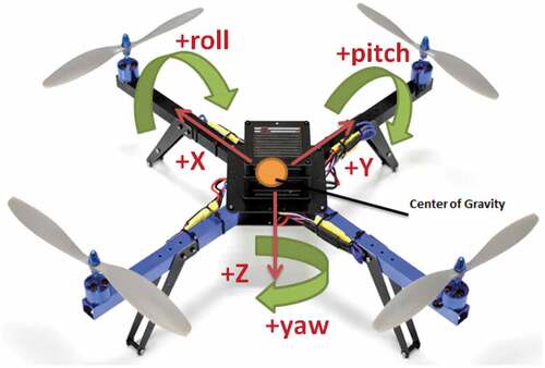
First of all, the coordinate frame has to be established. There are several coordinate systems used in aviation. Each one of them has its own advantages and disadvantages and is used accordingly. However, this project uses only one such system, namely the body axis system (Yechout et al. 2003). It is defined as follows:

• The coordinate system is fixed to the aircraft with its origin at the aircraft’s center of gravity (CG).

• The x axis is defined out of the nose of the aircraft.

• The y axis is defined out of the right wing of the aircraft.

• The z axis is defined as down through the bottom of the aircraft.

Figure 1 shows an example of a body axis coordinate system.

Figure 1. Body axis coordinate system

Quadrotor Control

A quadrotor is comprised of a thin cross structure with four propellers at its ends. Unlike a helicopter, the quadrotor does not require a tail rotor, due to the four-propeller cross configuration. Front and rear propellers rotate in a clockwise direction, while right and left propellers spin in the opposite (counter-clockwise) direction. Control of a quadrotor is performed by changing the rotation rate and thus the thrust of each rotor individually. Although control is achieved through changing rotation rates of individual motors, this approach is very counterintuitive for humans. Due to this reason, four so-called channels are used, namely throttle, roll, pitch, and yaw.

Throttle (U1): The throttle channel controls the overall amount of thrust generated by all four motors combined. Thus, changes in it result in a proportional change in the rotation rates of all four propellers. This is the only channel that controls the quadrotor’s linear acceleration and is mostly used to change altitude.

Roll (U2): The roll channel provides a means to create and control a tilt between the right and left rotors. This is achieved by increasing the rotation speed of the left propeller and decreasing the speed of the right one by exactly the same amount or vice versa. It is important to notice that overall thrust remains the same; thus, there is no linear acceleration produced.

Pitch (U3): The pitch channel is similar to roll, the difference being that it controls the tilt between the front and rear propellers. Everything else is the same.

Yaw (U4): The yaw channel allows the quadrotor to rotate in the horizontal plane. This is achieved by increasing the rotation rates of two propellers which either rotate clockwise or counter-clockwise, depending on the desired direction of rotation. To maintain overall thrust, this action has to be accompanied by an equivalent decrease in the remaining two propellers.

Experimental Setup and Procedure

This section presents the approach used to identify quadrotor attitude dynamics.

System Overview

The main goal of this paper is to identify pitch, roll and yaw dynamics of a quadrotor. Figure 2 shows the quadrotor used for this purpose.

Figure 2. Quadrotor

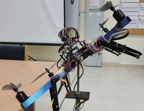
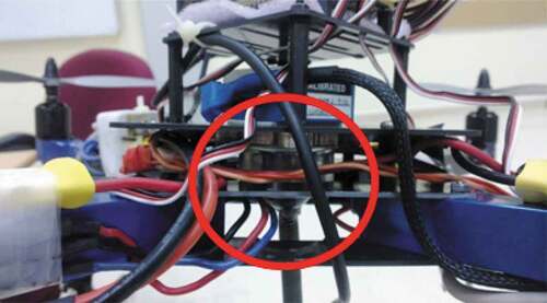
The most common practice is to find a relationship between input commands and angular rates, as done in Bresciani (2008). Thus, the output of a model should be the rate of change of the angles rather than the angles themselves. Dynamics of the fourth degree of freedom (DOF), namely z-axis acceleration, present little interest, because they correspond to a first-order linear system and are decoupled from the other DOFs. Identifying angle rates separately from z acceleration has one more advantage. Quadrotors are inherently unstable, so flying them without any control loops is impossible. However, if the goal is to identify only the angular dynamics, a quadrotor can be placed on a test stand with a spherical joint. Such a joint eliminates three DOFs, namely translational motion in all three axes. Nevertheless, if certain conditions are met, the motion in the remaining three DOFs remains unaffected. Obviously, the first condition is friction is kept as small as possible. The second one is that axis of rotation of the joint must be placed as close to the CG of the quadrotor as possible. Failing to meet this condition results in identifying a completely different system, because the moment of inertia changes in accordance with the parallel axis theorem. The red circle in Figure 3 shows the joint and its connection to the quadrotor.

Figure 3. Spherical joint

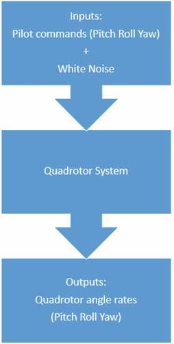
The most important part of system identification is clearly defining the inputs and outputs of the system. To do that, a good understanding of the general flow of information in the system is required. From this point of view, a quadrotor can be viewed in the following way: First of all, a human pilot generates a command, which he would like to send. After that, he inputs this command into a remote control (RC) transmitter, usually, by manipulating control sticks of the RC. The transmitter is linked to an RC receiver onboard the quadrotor. Receiving a radio signal results in the receiver generating an output electrical signal. This electrical signal is read by a microcontroller which performs the channel mixing operation described previously. The result of the operation is an individual rate for each propeller. Later, these rates are sent to electrical speed controllers (ESCs), which in turn regulates the voltage applied to the motors. Changes in the voltage applied result in changes in the propellers’ angular rates. Finally, this leads to a change in the quadrotor’s motion. The diagram shown in Figure 4 illustrates the whole process inputs and outputs of the system. Ideally one would like to record the commands as the pilot inputs them into the RC transmitter. However, this is rather complicated and unnecessary. The radio communications are much faster than the mechanical part of the system. Neglecting it does not result in a noticeable loss of accuracy. Due to this, it is possible to record received commands on board the quadrotor. In contrast to the inputs of the system, outputs are much easier to define. As it was mentioned above, outputs are three angular rates. To summarize, the inputs are three commands (pitch, roll, yaw) received by the microcontroller and the outputs are three angular rates $\dot{p}\dot{r}\dot{q}$.

Figure 4. Inputs/outputs diagram

According to the basic principles of system identification, the input signal has to be independent of the output. Unfortunately, in the case of a quadrotor, this is impossible. The problem comes from the instability mentioned above. Quadrotors are inherently unstable and react to the inputs so quickly that even an experienced pilot will not be able to keep it upright even when it is fixed to a test stand. This also causes big challenges for a controller design. Due to this, it is a common practice to add dumping to the quadrotor axis. This is achieved by adding a feedback loop for angular rates. Figure 5 shows the feedback loop structure.

Figure 5. Axis damping feedback loop

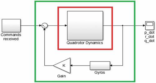
The red rectangle encloses the quadrotor’s raw dynamics. Meanwhile, the green rectangle shows raw dynamics with a feedback loop, which slows the quadrotor enough for a human to operate it. At this point, it is important to understand that a model is never a goal in itself, it is just a tool that allows certain goals to be achieved. In the case of an aircraft, a model is most commonly used to ease a controller design procedure. As long as gain K is not changed, one can use a new system defined by the green rectangle. This approach has been used and proven to be efficient in aviation and other fields (Menezes and Barreto 2008; Wu et al. 2014). The last part of this section describes the nature and characteristics of the input signals used to excite the system. As mentioned above, the receiver outputs four electrical signals, each one representing a control channel. This project is only concerned with three of them, namely pitch, roll and yaw. Each signal looks like a train of pulses and pulse width represents an angle of a control stick. Pulse width can vary from 1 ms to 2 ms. This is not ideal for mathematical manipulations and control applications because there is no negative region. Thus, the pulse width is shifted by −1.5 ms and ends up having values from −0.5 to 0.5. These are the values being recorded.

Hardware

This section provides the necessary description of the hardware used in the project. Most of the hardware used came from an Arducopter quadrotor. However, the microcontroller which comes with it has very limited data logging capabilities, due to a small amount of memory. In addition, the default telemetry can transmit data with a maximum rate of 15 Hz which is not good enough for system identification, which is the goal. Due to these reasons, a Beagle Bone White (BBW) embedded PC as a microcontroller is used. Unfortunately, replacing the ardupilot means losing its navigation system, so it is replaced by a MIDG IIC, which provides a full navigation solution. In addition to that, the arducopter does not include any radio controls. Thus, a Futaba 8 channel radio transmitter and receiver are used. Below is a complete list of hardware used in the project.

Arducopter components:

• The frame

• Four 12 V DC brushless motors

• 4 ESC

• Battery 12 V

• Power distribution board (Provides +12 V and +5 V output)

• Newly introduced components:

• BBW

  a) Processor 720MHz AM 3359 ARM (Texas Instruments)

  b) Power supply 5V (which is provided by the PDB mentioned above)

  c) 4 serial communication ports (1 required for MIDG)

  d) 66 GPIO pins (7 required for radio receiver, 4 required for ESCs)

  e) Easy 4GB uSD card access (useful for data logging)

• MIDG IIC

  a) Sampling rate 50 Hz

  b) Communication via serial RS-232 max 50 Hz

  c) Power supply 10-32V (can be handled by the battery)

• Futaba RC Tx and Rx

  a) 8 channel

  b) 2.4 GHz

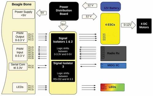
The last component needed for the project is a printed circuit board (PCB) that provides interfacing between the BBW and the rest of the electronics involved. BBW utilizes the TTL 3.3 standard. This means the maximum voltage for any input/output pin is 3.3 V. Older electronics utilize the TTL 5 standard, meaning logic levels are between 0 and +5 V. The PCB relies on the use of signal isolators to shift logic levels. On top of that, PCB has three LEDs connected to BBW GPIOs for a basic HMI. Figure 6 presents a pin diagram of the entire system.

Figure 6. Pin diagram

Software

A BBW is an embedded PC. The default OS shipped with the BBW is Linux Angstrom; a distribution of Linux specifically designed for embedded applications. Due to that, it is lighter and optimized for lower power consumption. This means that coding for a BBW is slightly different from coding for an ordinary microprocessor with no OS. However, the basic concepts are the same. There is a list of basic things one needs to be able to do for any embedded project. The list includes pin muxing, GPIO manipulation, PWM generation and acquisition. First of all, one has to be able to manipulate the pins’ mux settings. Most of the pins in a microprocessor are multiplexed. Thus, they can be used in several different ways, and a programmer has to specify how a pin should be used. Usually, this is done by putting some value into a specific register responsible for muxing. When working with an OS, one does not have direct access to registers or interrupts. However, Linux has directories to which values can be written and then passed to the registers by the OS itself. Actually, every single pin has a directory associated with it. Each one of those directories can be assigned a value, which determines the mode of a particular pin. A full list of all available modes can be found in the Beagle Bone manual. A more detailed description of the value computation procedure is provided in the AM335x technical manual.

The second step is to manipulate the GPIO pins. When working directly with hardware, all that needs to be done is configured the mux register to put a pin into a GPIO mode and then simply put the required values into in/out and high/low bits of configuration registers. As mentioned previously, an OS does not give direct access to the registers. Assuming muxing was done previously, the first thing that has to be done is to export the pin by sending the pin number to the export directory. The procedure tells the kernel that the OS wants to work with this particular GPIO pin. After a pin is exported, its directory appears in the GPIO class directory and can be accessed. Inside the pin’s directory, one can find directories corresponding to the pin’s direction (in/out) and value (high/low), thus achieving the goal.

The first two parts are rather easy. However, when one attempting to acquire a high-frequency signal, the problem of latency arises. When an application needs to communicate with a hardware, it has to communicate with the OS first. The OS in turn has to communicate with the kernel, which has direct access to the hardware. Then, all have to go all the way back. This causes a significant delay, making even an acquisition of a 50 Hz PWM signal impossible. However, there is a way around this issue. The microprocessor used in a BBW is an AM 3359 ARM. These types of microprocessors have an internal subdivision into several processors. While the main part of the microprocessor runs at 720 MHz and has an OS installed on it, there are two other parts called programmable real-time units (PRUs). These parts run only at 200 MHz, but they do not have any OS installed. This allows them direct access to the hardware and thus makes them much faster when it comes to hardware manipulation. This is different from both the physical and logical separations in ordinary computers and does not allow full-scale multiprocessing. Unfortunately, there is a drawback. Since there is no OS on either of the PRUs, they cannot run executable files. This means that one cannot compile a C code and make a PRU run it. Due to this, one has to provide a PRU with a .bin file. There are several ways to make it. For example, one can code it in C and then use an IDE which has the tools to turn it into machine code. That is exactly what MPLAB does for PIC microcontrollers. However, each family of microprocessor requires a different set of tools, which are quite expensive and difficult to acquire. Due to that, a simpler approach was used. An assembly code was written in a text editor (like a notepad) and then compiled using the PASM software, provided by Texas Instruments. Communication between all three parts of the microprocessor is achieved through shared memory. Figure 7 depicts a portion of the AM335x technical manual (Texas Instruments [2013]) showing PRU memory location in a memory map.

Figure 7. Part of AM335x family memory map (AM335x ARM cortex – A8 microprocessors (MPUs) technical reference manual 2013, 176)

As a matter of fact, access to the memory is controlled internally and the programmer does not have to bother implementing any kind of protocol. On top of that, Texas Instruments provides a C library specially created to work with PRUs. It is called prussdrv.c, prussdrv.h.

Input Signal Specifications

The data gathering process consists of applying an input to the system and observing the output. All inputs and outputs were discussed earlier. However, it was not specified what shape the input signal should have. Initially, the input used in the experiment consisted only of a command being sent by a pilot. However, there is a problem with that, namely the frequency content of the input signal. For good system identification, all of the system’s frequencies have to be exited. But, no matter how good the pilot is, a signal with frequencies higher than 2–3 Hz cannot be produced. This was solved by adding a pseudo-random component to the signal in the software. With a pseudo-random component, the input signal has all the frequencies from DC to 25 Hz. At the same time, all the pilot has to do is to keep a quadrotor upright to prevent it from hitting the boundaries of the spherical joint. As discussed previously, all the inputs and outputs are recorded onboard and then downloaded to the host PC. Because the MIDG output hardly has any noise in it, the obtained data is not filtered. However, sometimes the packets sent by the MIDG get lost or corrupted. The amount of information loss due to this is very small and can be neglected. Nevertheless, this results in data not being equally sampled, while most system identification algorithms rely on the assumption that it is. So, a MATLAB script was written to find such places in the log file and restore them by interpolating the data.

Quadrotor System Identification

Continuous Time Transfer Functions

The most common approach toward creating a model in avionics is gray-box modeling (Bresciani 2008). This method assumes that the structure of a model is known; it can either be derived from the first principles or determined by trial and error. However, the parameters of the model have to be found through the use of some estimation algorithm (Bosch and Van der Klauw 1994). The most basic way to represent a system is to acquire its transfer function by taking the Laplace transform of differential equations describing the system. Transfer function models describe the relationship between the inputs and outputs of a system using a ratio of polynomials (Franklin, Powell, and Emami-Naeini 2009). The model order is equal to the order of the denominator polynomial. The roots of the denominator polynomial are referred to as the model poles, and the roots of the numerator polynomial are referred to as the model zeros. The parameters of a transfer function model are its poles and zeros (Close, Frederick, and Newell 2002). It is very common to assume that the relation between pilot commands and Euler angles’ rates is that of a second-order underdamped system. This assumption is based on the following facts. First of all, it can be shown that the speed of any propeller connected to a DC-motor can be described by the following first-order differential equation (Bresciani 2008):

(1) ${\dot{\omega }}_p=A_p{\omega }_p+B_{p}v+C_p$(1)

where:

${\omega }_p$ – propeller speed

$v$ – voltage applied to the motor

$A_p,B_p,C_p$ – linearization coefficients

It is important to point out that voltage applied to the motor is a result of an operation called channel mixing. The operation consists only of linear equations. Thus, the relation between pilot commands and voltages applied to the motors are linear and not differential. It has to be mentioned that this is only true if one assumes that ESCs have no dynamics. At the same time, the difference in the propellers’ angular velocities produces torque acting on the quadrotor. Thus, if one defines a generalized force vector (Λ) as:

(2) $\mathrm{\Lambda }=\left[F_x{F}_y{F}_z{\tau }_x{\tau }_y{\tau }_z\right]$(2)

It can be shown that generic dynamics of 6 DOF can be written in a matrix form as follows (Bresciani 2008):

(3) $M_B\dot{V}+C_{B}V=\mathrm{\Lambda }$(3)

where:

$\dot{V}$ – generalized acceleration of a body

$M_B$ – system inertia matrix

$C_B$ – Coriolis-centripetal matrix

If one combines (1) and (3) making use of (2), a set of second-order differential equations is obtained. Due to this fact, it makes sense to assume a second-order relation between pilot commands and angle rates. Thus, the transfer function should have the form shown by (4).

(4) $H\left(s\right)=\frac{Y\left(s\right)}{X\left(s\right)}=\frac{K}{\left(1+2T_{\omega }\zeta s+T_{\omega }^2{s}^2\right)}$(4)

where:

$Y\left(s\right)$ – angle rate

$X\left(s\right)$ – pilot command

K – DC gain

$T_{\omega }$- inverse of corner frequency

$\zeta$ – damping factor

However, parameters K, $T_{\omega }$, $\zeta$ remain unknown and have to be estimated. Some obvious drawbacks of the approach are linearization and decoupling. A classical Laplace transform used to obtain transfer functions from differential equations assumes a system is linear and time-invariant. Thus, a transfer function obtained through an estimation process will be a linearization of a system around some point of operation (Bresciani 2008; Ge et al. 2009). In this particular case, it will be the hovering point, because during the experiment the quadrotor was mostly kept upright. The second issue mentioned is decoupling. This happens because, by definition, transfer functions represent a relation between one particular input and one particular output. Thus, to obtain a truly MIMO system, one has to find all possible transfer functions. However, this is out of this project scope. The method being discussed is mostly used to show that the system is nonlinear and has a significant amount of coupling.

Nonlinear Autoregressive Network with Exogenous Inputs (NARX)

The nonlinear autoregressive network with exogenous inputs (NARX) is a type of recurrent dynamic network that is frequently used for estimating time-series (Menezes and Barreto 2008; Wang and Song 2014; Wong and Worden 2007). The most distinctive feature of a NARX network is that it has a feedback enclosing several layers of the network. Thus, the equation describing a NARX network is:

$y\left(t\right)=f(y\left(t-1\right),y\left(t-2\right),\dots ,y\left(t-m_y\right),$

(5) $u\left(t\right),u\left(t-1\right),\dots ,u\left(t-k_u\right))$(5)

where: $y\left(t\right)$ – network output at time t and $u\left(t\right)$ – network input at time t.

As can be seen, every value of the dependent output signal y(t) is regressed on previous values of the output signal and previous values of an independent (exogenous) input signal. This makes NARX networks capable of nonlinear dynamic system modeling (Pisoni et al. 2009; Zemouri, Gouriveau, and Zerhouni 2010). However, using the feedback feature of NARX networks during the training phase is unjustified (Menezes and Barreto 2008; Wang and Song 2014). First of all, the true output is available during training. Thus, the network can be supplied with much more accurate inputs. In addition to that, a static backpropagation learning algorithm cannot be used. Due to these two facts, NARX networks are usually converted from parallel, shown in Figure 8 to series-parallel, shown in Figure 9 architecture for training.

Figure 8. NARX series-parallel architecture (MATLAB 2013a. 2013. MathWorks)

Figure 9. NARX parallel architecture (MATLAB 2013a. 2013. MathWorks)

As mentioned above, Series-Parallel architecture allows using static learning algorithms. One of such algorithms is Levenberg-Marquardt backpropagation. As well as quasi-Newton methods, the Levenberg-Marquardt algorithm can approach second-order training speed, while not needing to compute the Hessian matrix (Menezes and Barreto 2008). The algorithm relies on the fact that if a performance function has the form of a sum of squares, then the Hessian matrix H can be approximated as:

(6) $H=J^{T}J$(6)

and the gradient $\mathrm{\nabla }$ can be computed as:

(7) $\mathrm{\nabla }=J^{T}e$(7)

In (6) and (7) J is the Jacobian matrix. This matrix consists of the first derivatives of the errors with respect to weights and biases. e is simply a network error vector. Approximations mentioned above are then used in a Newton-like update of the weights:

(8) $w_{n+1}=w_n-{\left[J^{T}J+\mu I\right]}^{-1}{J}^{T}e$(8)

As explained previously, this method relies on the assumption that performance is a mean or sum of squared errors. Thus, a NARX trained with this method has to have either the MSE or SSE performance function. This project used the MSE function which is calculated using the following formula:

(9) $MSE=\frac{1}{N}\sum _{k=1}^N{\left(y-\hat{y}\right)}^2\left(k\right)$(9)

The NARX network was trained in the Series-Parallel mode and then converted to Parallel architecture for testing.

Experimental Results

The system identification of the quadrotor dynamics has been performed using a data set of 12500 samples, equally spaced over a period of 250 seconds. The following transfer functions were obtained:

Pitch Rate:

$H_{1,1}\left(s\right)=\frac{\dot{p}\left(s\right)}{u_p\left(s\right)}=\frac{334}{0.009467s^2+0.06256s+1}$

Roll Rate:

$H_{2,2}\left(s\right)=\frac{\dot{r}(s)}{u_r\left(s\right)}=\frac{299.8}{0.01426s^2+0.07517s+1}$

Yaw Rate:

$H_{3,3}\left(s\right)=\frac{\dot{q}\left(s\right)}{u_q\left(s\right)}=\frac{350}{0.01823s^2+1.015s+1}$

Figures 10, 11 and 12 below, show measure and modeled angle rates of the quadrotor.

Figure 10. Modeling performance of pitch rate transfer function

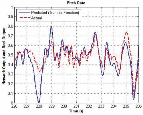
Figure 11. Modeling performance of roll rate transfer function

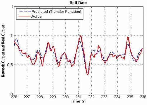
Figure 12. Modeling performance of yaw rate transfer function

Table 1 summarizes the results of using continuous time transfer function to model the quadrotor dynamics.

Table 1. CTTF results

Angle rate	MSE	VAF (%)	Correlation Coefficient	Outlier ratio
Pitch rate	0.0106	18.6	0.75	0.07
Roll rate	0.0054	65.1	0.77	0.04
Yaw rate	0.0772	5.33	0.61	0.04

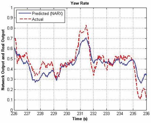
The same data set is used to train and validate a NARX network. Below, measured and predicted outputs are shown in Figures 13, 14 and 15.

Table 2 summarizes the results of using continuous time transfer function to model the quadrotor dynamics.

Table 2. NARX results

Angle rate	MSE	VAF (%)	Correlation Coefficient	Outlier ratio
Pitch rate	0.0077	54.4	0.74	0.07
Roll rate	0.0047	72.9	0.87	0.04
Yaw rate	0.0112	69.3	0.86	0.08

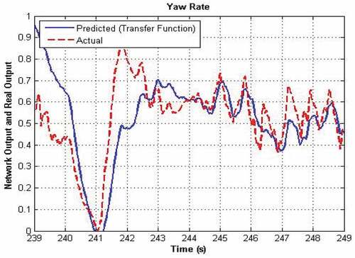
As it was stated in the theory section, the number of delays used in the network has to be found experimentally. This is done by increasing the number of delays until the improvement becomes insignificant. Figures 16, 17 and 18 show the relation between the number of delays used and network performance.

Figure 13. Modeling performance of the NARX model of pitch rate during testing

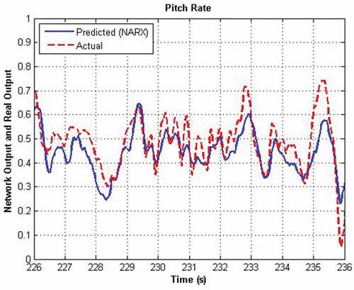
Figure 14. Modeling performance of the NARX model of roll rate during testing

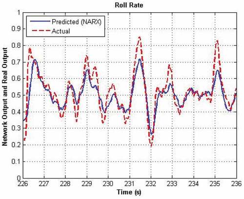
Figure 15. Modeling performance of the NARX model of yaw rate during testing

The results presented above show that the NARX network managed to model the system. NARX model performance is much better than that of a transfer function. This is mostly because NARX can easily incorporate any kind of coupling.

Results Validation

Data Set Dependency

Results obtained from data-driven techniques heavily depend on the data provided. Thus, it is a common practice to perform some kind of validation after the results are obtained to show that they are not data-dependent. Usually, this is done by shifting the testing window while using the same data set. As mentioned above, initially 200 seconds of data were divided into a training set (50–200 seconds), and a testing set (200–250) seconds. The results obtained with this division are reported in Section 5. Later, the training set was changed to 100–250 seconds, and the testing set was changed to 50–100 seconds, and the whole procedure was repeated. Needless to say, this is not required for classical CTTF, because windows of 3 seconds were used to estimate their coefficients. Thus, the coefficients are average values already. The results obtained with the new data set division are presented in Table 3.

Table 3. NARX results

Angle rate	MSE	VAF (%)	Correlation Coefficient	Outlier ratio
Pitch rate	0.0064	54.17%	0.77	0.06
Roll rate	0.0048	73.8%	0.86	0.06
Yaw rate	0.0050	50.6%	0.72	0.07

It can be seen that the change caused by using a different data division is rather insignificant and most importantly inconsistent, leading to a slight improvement in some cases and deterioration in others. This illustrates the independence of the results obtained earlier from a particular portion of data being used.

Data Set Size Dependency

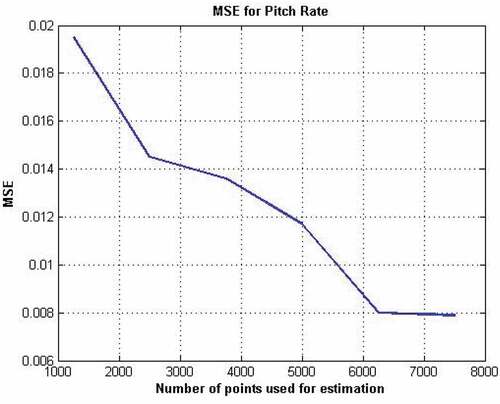
Another important criterion is the amount of data provided. It is obvious that for the techniques used in this project, the size of the data set is of major importance. It is also obvious that after a certain point, further increases in the amount of data will not yield a significant improvement in the model accuracy. Thus, a check can be performed to see if the data set size was sufficiently big. This is done by increasing the amount of training data and monitoring the performance of the obtained models. In this project, the MSE was used for performance evaluation. Table 4 shows the change in MSE due to the increase in the training data set for NARX.

Table 4. NARX MSE

Data Used	1250	2500	3750	5000	6250	7500
Pitch Rate	0.02	0.015	0.014	0.012	0.008	0.008
Roll Rate	0.014	0.011	0.007	0.005	0.004	0.004
Yaw Rate	0.024	0.013	0.012	0.012	0.007	0.006

The three plots below show a relation between MSE and the amount of data used for training for each output of the model.

It can be seen that in each case MSE shows a rapid improvement in the beginning followed by a huge decrease in sensitivity to an increase in training set size. This illustrates that further increases in the amount of data provided to the network for training will not result in any significant improvement.

Conclusion

This paper has presented an experimental setup that allowed to acquire data for system identification purposes. We have successfully modeled the system using NARX ANN. Observing the relation between MSE and number of data points, shown in Figure 19, 20, 21, allows to conclude that sufficient amount of data was gathered to train the networks. Figures 16, 17 and 18 show that the number of delays was adequate and allowed networks to capture the system dynamics. From Figures 13, 14 and 15, we can observe that the identified dynamic model performs well. At the same time, Tables 1 and 2 show that using NARX results in lower MSE and higher correlation coefficient than the transfer function model. It is important to point out that improvement is consistent among all three angle rates. The model obtained can be used in controllers that require a system model. We expect this approach to be adoptable to any kind of rotary-wing UAVs, like hexarotors etc. The future work will be focused on improving the experimental setup to obtain higher quality data sets. Moreover, an attempt should be made to use the model for controller design or in a model predictive controller.

Figure 16. Number of delays vs MSE for pitch rate

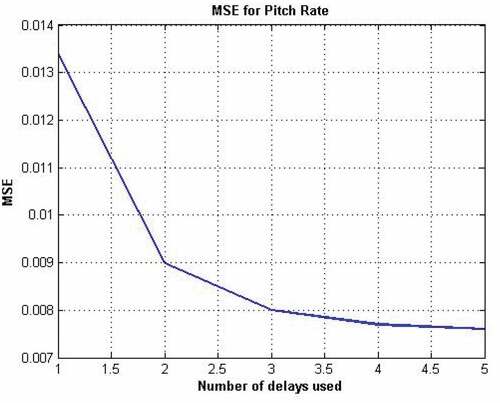
Figure 17. Number of delays vs MSE for roll rate

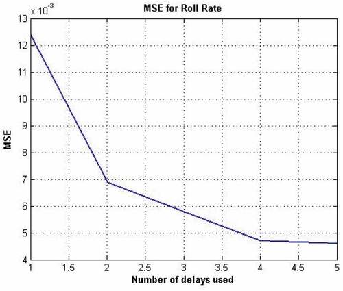
Figure 18. Number of delays vs MSE for yaw rate

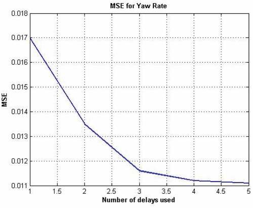
Figure 19. MSE for yaw rate vs training set size

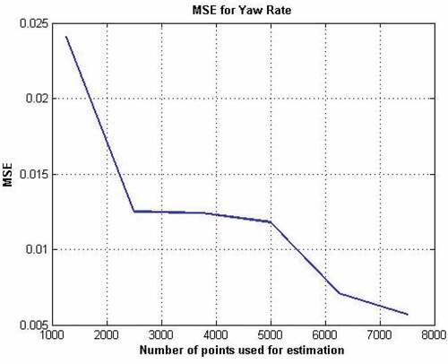
Figure 20. MSE for roll rate vs training set size

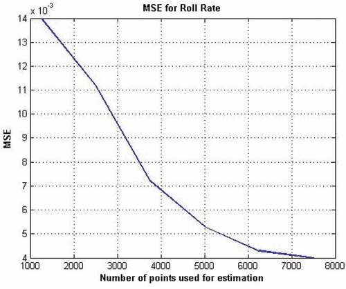
Figure 21. MSE for pitch rate vs training set size

References

- Altan, A., O. Aslan, and R. Hacioglu. 2018. Real-time control based on NARX neural network of hexarotor UAV with load transporting system for path tracking. 6th International Conference on Control Engineering & Information Technology (CEIT), Istanbul, Davutpasa Convention Center.
- Assaleh, K., M. AlHamaydeh, and I. Choudhary. 2015. Modeling nonlinear behavior of buckling-restrained braces via different artificial intelligence methods. Applied Soft Computing 37:923–38. doi:10.1016/j.asoc.2015.09.014.
- Bayat, S., H. N. Pishkenari, and H. Salarieh. 2019. Observer design for a nano-positioning system using neural, fuzzy and ANFIS networks. Mechatronics 59:10–24. doi:10.1016/j.mechatronics.2019.02.007.
- Bergamasco, M., and M. Lovera. 2014. Identification of linear models for the dynamics of a hovering quadrotor. Control System Technology 22(5):1696–1707.
- Bosch, P. P., and A. C. Van der Klauw. 1994. Modeling, identification and simulation of dynamical systems. Florida: CRC Press.
- Bresciani, T. 2008. Modelling, identification and control of a quadrotor helicopter. Master thesis, Lund University.
- Close, C. M., D. K. Frederick, and J. C. Newell. 2002. Modeling and analysis of dynamic systems. 3 ed. New York: Wiley.
- Elsamanty, M., A. Khalifa, M. Fanni, A. Ramadan, and A. Abo-Ismail. 2013. Methodology for identifying quadrotor parameters, attitude estimation and control. Advanced Intelligent Mechatronics (AIM), 2013 IEEE/ASME International Conference, Wollongong, University of Wollongong.
- Franklin, G. F., J. D. Powell, and A. Emami-Naeini. 2009. Feedback control of dynamic systems. Addison-Wesley Reading. : New Jersey: Pearson Prentice Hall.
- Ge, H.-W., W.-L. Du, F. Qian, and Y.-C. Liang. 2009. Identification and control of nonlinear systems by a time-delay recurrent neural network. Neurocomputing 72:2857–64. doi:10.1016/j.neucom.2008.06.030.
- Gharajeh, M. S., and H. J. Jond. 2020. Hybrid global positioning system-adaptive neuro-fuzzy inference system based autonomous mobile robot navigation. Robotics and Autonomous Systems 134:103669. doi:10.1016/j.robot.2020.103669.
- Granados-Bolanos, S., A. Quesada-Roman, and G. E. Alvarado. 2020. Low-cost UAV applications in dynamic tropical volcanic landforms. Journal of Volcanology and Geothermal Research 107143. doi:10.1016/j.jvolgeores.2020.107143.
- Hosovsky, A., J. Pitel, K. Zidek, M. Tothova, J. Sarosi, and L. Cveticanin. 2016. Dynamic characterization and simulation of two-link soft robot arm with pneumatic muscles. Mechanism and Machine Theory 103:98–116. doi:10.1016/j.mechmachtheory.2016.04.013.
- Jaradat, M. A. K., and F. A. H. Mamoun. 2016. Non-linear autoregressive delay-dependent INS/GPS navigation system using neural networks. IEEE Sensors Journal 17 (4):1105–15. doi:10.1109/JSEN.2016.2642040.
- Kim, J., M. S. Kang, and S. Park. 2009. Accurate modeling and robust hovering control for a quad-rotor VTOL aircraft. Selected Papers from the 2nd International Symposium on UAVs 20:9–26.
- Kislitsyna, A. I., and G. F. Malykhina. 2017. Simulation of an on-the-fly measuring system of a descent module under uncertainty of the lunar-surface composition. St. Petersburg Polytechnical University Journal: Physics and Mathematics 3:199–209. doi:10.1016/j.spjpm.2017.09.003.
- MATLAB. 2013a. 2013. MathWorks.
- Menezes, J. M. P., and G. A. Barreto. 2008. Long-term time series prediction with the NARX network: An empirical evaluation. Neurocomputing 71:3335–43. doi:10.1016/j.neucom.2008.01.030.
- Nguyen, N. S., V. K. Cao, and H. P. Huy Anh. 2017. A novel adaptive feed-forward-PID controller of a SCARA parallel robot using pneumatic artificial muscle actuator based on neural network and modified differential evolution algorithm. Robotics and Autonomous Systems 96:65–80. doi:10.1016/j.robot.2017.06.012.
- Parvaresh, A., and S. A. A. Moosavian. 2019. Linear vs. Nonlinear Modeling of Continuum Robotic Arms Using Data-Driven Method. 7th International Conference on Robotics and Mechatronics (ICRoM), Iran, Tehran 457–62, Nov.
- Pisoni, E., M. Farina, C. Carnevale, and L. Piroddi. 2009. Forecasting peak air pollution levels using NARX models. Engineering Applications of Artificial Intelligence 22:593–602. doi:10.1016/j.engappai.2009.04.002.
- Pounds, P., R. Mahony, and P. Corke. 2006. Modelling and control of a quad-rotor robot. Proceedings Australasian Conference on Robotics and Automation 2006, New Zealand, Auckland.
- Pounds, P., R. Mahony, and P. Corke. 2010. Modelling and control of a large quadrotor robot. Control Engineering Practice 18:691–99. doi:10.1016/j.conengprac.2010.02.008.
- Qianying, L. 2014. Grey-box system identification of a quadrotor unmanned aerial vehicle.
- Sezginer, K., and C. Kasnakoglu. 2019. Autonomous navigation of an aircraft using a NARX recurrent neural network. 11th International Conference on Electrical and Electronics Engineering (ELECO), Turkey, Bursa 895–99 November.
- Texas Instruments. 2013. AM335x ARM cortex –A8 microprocessors (MPUs) technical reference manual. 176.
- Wang, H., and G. Song. 2014. Innovative NARX recurrent neural network model for ultra-thin shape memory alloy wire. Neurocomputing 134:289–95. doi:10.1016/j.neucom.2013.09.050.
- Wilmer, A. R., Z. Q. Leong, H. D. Nguyen, and S. G. Jayasinghe. 2020. Machine learning post processing of underwater vehicle pressure sensor array for speed measurement. Ocean Engineering 213:107771. doi:10.1016/j.oceaneng.2020.107771.
- Wong, C., and K. Worden. 2007. Generalised NARX shunting neural network modelling of friction. Mechanical Systems and Signal Processing 21:553–72. doi:10.1016/j.ymssp.2005.08.029.
- Wu, J., H. Peng, Q. Chen, and X. Peng. 2014. Modeling and control approach to a distinctive quadrotor helicopter. ISA transactions 53:173–85. doi:10.1016/j.isatra.2013.08.010.
- Xiaodong, Z., L. Xiaoli, W. Kang, and L. Yanjun. 2014. A survey of modelling and identification of quadrotor robot. Abstract and Applied Analysis 2014:1–16.
- Yechout, T. R., S. L. Morris, D. E. Bossert, and W. F. Hallgren. 2003. Introduction to aircraft flight mechanics: Performance, static stability, dynamic stability, and classical feedback control. Reston, VA: American Institute of Aeronautics and Astronautics.
- Yuan, H., C. Xiao, Y. Wang, X. Peng, Y. Wen, and Q. Li. 2020. Maritime vessel emission monitoring by an UAV gas sensor system. Ocean Engineering 128:108206. doi:10.1016/j.oceaneng.2020.108206.
- Zemouri, R., R. Gouriveau, and N. Zerhouni. 2010. Defining and applying prediction performance metrics on a recurrent NARX time series model. Neurocomputing 73:2506–21. doi:10.1016/j.neucom.2010.06.005.