A Comparative Study of Artificial Intelligence Models for Predicting Interior Illuminance

ABSTRACT

Thanks to the recent advances in computer technology, many building energy performance simulation tools have been developed in the current market. Designers and architects are interested in working on this topic in the early phases of the project. However, effective energy solutions are computationally expensive. As a result, having a comprehensive insight into the project conditions in the early phases of the work is a vital issue. The present study aimed to propose an artificial intelligence (Al) model to generate a reasonably accurate estimate in a short time. To this end, four machine learning models and one artificial neural network (ANN) are selected and their results are compared to assess their capabilities in energy performance estimation. This study investigates the influence of the exterior louver design on the interior energy performance of a structure. A specific dataset is generated and tested on four powerful regression models (i.e., polynomial Linear Regression, Random Forests (RF), Decision Tree (DT), and Support Vector Regression (SVR)) and one Artificial Neural Network (ANN). Finally, a comparative analysis is presented. The findings of this research support the use of machine learning tools and ANNs as a convenient and accurate strategy for predicting building parameters.

Introduction

The energy performance of buildings (EPB) has been the subject of intense research because of growing concern about energy dissipation and associated perennial negative environmental impact (Kirimtat et al. 2019). According to reports, there has been a steady global growth in building energy consumption (BEC) over the past decades (da Graça Carvalho 2012). It seems that architecture is the only solution for minimizing energy consumption in BEC (Kirimtat et al. 2016a). Consequently, the construction of a more energy-efficient building can be considered a solution to meet the growing demand for extra energy (Khoroshiltseva, Slanzi, and Poli 2016).

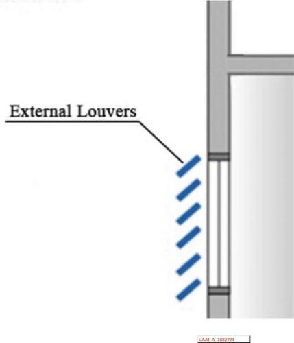
One of these architectural solutions is the use of louver in the early design phases. Louvers are essential for summer seasons to prevent solar radiation while allowing it to enter the building in the cold seasons. Louvers also decrease the operating costs, specifically in cooling and heating systems, by saving a significant amount of energy without blocking the daylight entirely (Kirimtat et al. 2019). According to Figure 1, the multifunctional external louvers are mounted on the facade at a certain angle, which changes with the motion of the sun during the daytime. Mounting the panels horizontally or vertically depends on the climatic conditions. For instance, in hot and dry climates, the panels should be mounted horizontally on the southern facade, which is the case in this paper (Kirimtat et al. 2019).

Figure 1. Schematic drawing of a louver system for building

Nowadays, building energy-consumption simulation tools are commonly used for designing and implementing energy-efficient buildings by assessing or predicting energy consumption. In practice, the simulation findings often produce accurate results (Wagdy et al. 2017; Yao 2014). Simulation tools are commonly used in different areas as they allow visual examination of parameters that are very difficult, if not impossible (Katsifaraki, Bueno, and Kuhn 2017). For more information and comparison of building and daylighting simulation tools, see Ayoub (2020) and Davoodi et al. (2019).

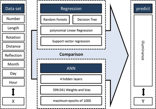
This study aimed to analyze the findings statistically to obtain a profound insight into the fundamental characteristics of input and output factors for an artificial neural network (ANN) to provide a reasonably accurate estimate in a short time. In this way, robust classical regression, state-of-the-art nonlinear and nonparametric machine learning tools (random forests, SVR, and Decision Tree), and ANNs are used to map the input variables to the output variable illuminance. In the next section, by varying the hyperparameters of each method, it is tried to achieve the best accuracy and the least Mean Squared Error (MSE) rate to compare all methods with an appropriate criterion. Finally, the most optimal methods for predicting the objective function (i.e.,illumination) are presented according to their success rate (Figure 2).

Figure 2. Procedure of this article

Background

Daylighting is one of the fundamental ingredients of passive solar building design that must be accurately estimated. Shading device and louver are among the best-integrated components of the building and facades to protect the interior from overheating and providing adequate daylight levels (Kirimtat et al. 2016a). The critical question of this study is how the designer should decide the formal specifics of the louvers (Choi et al. 2014). Information about designing good performing louvers is rather limited (Kirimtat et al. 2019). Typically, the most important factor considered when designing the louvers is the architect’s intuitive design (Choi et al. 2013).

Numerous studies have analyzed the energy performances of louver systems (Khaled et al. 2017; Kirimtat et al. 2016b; Li, Qu, and Peng 2016; Skarning et al. 2017; Valladares-Rendón, Schmid, and Lo 2017; Yun, Park, and Kim 2017). Kirimtat et al. (2019) examined different types of shading devices to find an appropriate design according to the climatic characteristics, the type of facade, and the position of the building. In another article, Choi et al. (2014) used five variables to design different kinds of louver systems.

In general, modeling a complex architectural system is a difficult task. A key requirement to solve this problem is developing a standard assessment model to support the decision-making process (Tregenza and Mardaljevic 2018). Different methodologies are employed by architects and designers to model daylighting and its effect on buildings and to support their decisions during different stages of design (Tregenza 2017). Daylight simulations provide designers with the ability to compare and optimize design alternatives to promote visual and thermal comfort for the occupants (Nasrollahi and Shokri 2016) while exploiting energy-efficient techniques (Amasyali and El-Gohary 2018). Optimization provides the opportunity to explore a great number of design solutions efficiently.

In recent years, the expansion of parametric design, building performance simulation, and optimization technologies has allowed transforming the building design challenges into the mathematical domain (Fang and Cho 2019). The process of building performance optimization includes building simulation programs and the optimization engine that include various optimization algorithms (Nguyen, Reiter, and Rigo 2014). Usually, two types of inputs are needed for an optimization process: variables and objective functions. Variables are the values controlling the building design properties. On the other hand, objective functions, which usually are calculated by simulation tools, are the building performance metrics (Aldawoud 2013; Machairas, Tsangrassoulis, and Axarli 2014; Tzempelikos and Chan 2016; Yao 2014).

During the early stages of building design, accurate prediction of indoor illuminance is considered among the most important factors in saving energy and costs associated with lighting (Kim and Kim 2019a). Over past decades, many attempts have been made to predict daylighting; e.g. diagrams, protractors, calculations, rules-of-thumb, and scale models under natural or artificial skies. The successive developments of computer architectures and specialized hardware have prompted the development of more advanced simulation tools (Schardl 2016).

The goal of most artificial intelligence approaches is to develop specific algorithms to improve the accuracy of results and modeling speed (Chou et al. 2015). Also, these tools can reduce the processing time by changing some building parameters during the design phase if properly trained. In general, artificial intelligence methods not only accelerate the optimization process but also increase the chance of finding an ideal solution through search space reduction (Su and Yan 2015). Therefore, many scientists use machine learning tools and rely on appropriate datasets to study the effect of various construction parameters such as compactness and specific factors such as energy consumption (Weerasuriya 2014). It is worth noting that due to a wide diversity of artificial intelligence models, benchmarking has rarely been applied to architectural design methods and tools (Gill, Summers, and Turner 2017).

Despite individual comparisons in the literature, there is tremendous variability between different artificial intelligence approaches (Summers, Eckert, and Goel 2017). In this regard, Manzan (2014) investigated a genetic optimization to realize a fixed shading system with an optimal geometry and lower energy consumption. Minimizing total energy consumption has been only the goal of design optimization. Zani et al. (2017) performed the computational analysis of a traditional type of static louver by integrating them into a single office facade through performing genetic algorithms in the optimization process. In similar projects, artificial intelligence models have been proposed for such energy challenges as power-to-heat options (Chou and Bui 2014; Lorenz et al. 2018).

In the present study, the louver topic in the field of energy is selected as a sample benchmark that can be generalized to other fields of energy. The exact formulation of the louver design is a difficult task due to several influential variables such as geographical location, weather condition, and shape (Choi et al. 2014). The current study is based on Choi and Lee’s work, who used those variables such as number, length, and rotation of louvers to investigate how they affect cooling and heating load (Choi et al. 2014). The dataset of this study consists of 5,812 samples that all share a constant variable of geographic location and some independent variables such as a month, day, hour, louver design parameters such as rotation, length, distance from the window, reflection, and the number of louvers. This study investigates the impact of eight input factors to measure the illuminance of the buildings, as the output variable. The motivation behind this research is to create a system that helps architects to make more accurate design decisions and to know its result. This paper specifically focuses on an artificial intelligence model to predict the illuminance at a reasonable time and accuracy. To this end, out of the great variety of artificial intelligence models, four models (i.e., polynomial Linear Regression, supporting vector machines (SVM), decision trees, and Random Forest (RF)) and artificial neural networks (ANNs) were selected to predict important matters in the EPB context. Moreover, their capabilities and the obtained results were compared to examine the capacity and accuracy of each in an example energy problem. To obtain this goal, a comparative study is carried out to identify the best AI predictive model for this field of research.

Research Approach

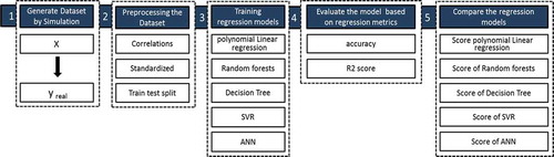
In this article, first, a dataset was obtained using simulation software and modifying attributes. Before beginning the coding process, the preprocessing steps were performed by examining the correlation between each input variable with another input variable, as well as each variable (input or output) with the output variable (illuminance). Next, the variables were normalized in the range of 1 to −1 such that to predict without prioritizing the variables. Afterward, the dataset is divided into training and testing batches using the mentioned values.

In this step, values from the output variable (y^{^}) are obtained for each machine learning tool (PLR, RF, SVR, and Decision tree), and artificial neural networks (ANNs). In the learning process, the error rates in each method were tried to be reduced compared to the real value (Y_real). In the final step, the standard techniques were evaluated by comparing their computational accuracy and prediction to present the best predictive model for our purpose (Figure 3).

Figure 3. Diagram of the present research structure and its six steps

Dataset

The following case study has two main aims. The first aim is to help designers to explore and discover louver alternatives and enable them to consider the numerous alternatives for the best design. The second aim is to use the case study to add information on the influence of various types of static and dynamic louvers on the internal illuminance of office space. As mentioned before, the proposed tool allows defining any type of dynamic measurement parameters according to the user’s needs.

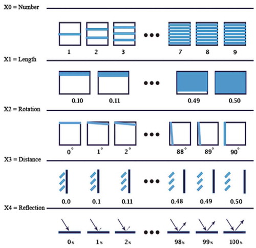
In our case, based on the geometry of the louvers, five independent variables are specified. The number of independent variables is suitable because the high number of independent variables blocks the training process. So, in addition to the stochastic approach of the optimization process, the high number of variables adds more uncertainty (Kirimtat et al. 2019). As a result, a parametric sensitivity test is used to examine these eight strict parameters: rotation, length, distance from the window, reflection, number of louvers, month, day, and hour. Figure 4 summarizes the researchinput and output variables, their mathematical representations, and their possible values.

Figure 4. Impact parameters in the Louver design

A simulation is conducted to validate the function of the parametric louver design system in the following phases: setting a building analysis; using the parametric louver design algorithm to determine the optimal louver shape; and predicting building illuminance with distinct louver shapes. In this paper, the presented tool for simulation is the Grasshopper platform for Rhino3D software and the Diva plugin for Grasshopper. One tool in the Rhino3D modeling environment for integrating validated Radiance/Daysim simulations is the Diva plugin (Grobman, Capeluto, and Auster 2016). DIVA can be used for the rapid visualization of daylight results from an architectural design model. This tool also enables us to easily examine different kinds of design variants for daylight (Jakubiec and Reinhart 2011).

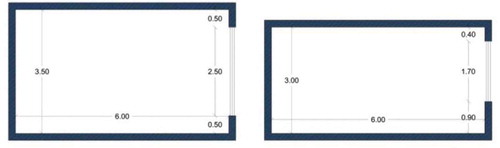
The characteristics of the studied office space for simulation at Grasshopper are as follows: 6 m × 3.5 m space area, 3 m height, and 1.7 × 2.5 window on the south side (Figure 5 and Table 1). The window size was estimated based on the 30% to 40% ratio of the window region to Tehran city’s internal wall. In this situation, the window can minimize energy consumption by providing daylight energy (Mahdavinejad et al. 2012). Eight construction parameters are used to describe 5812 simulated structures to comply with conventional mathematical notation and facilitate the assessment. Henceforth,these construction parameters are called input variables and denoted by X. We also record the amount of light for each building. These parameters will henceforth be called the output variable and denoted by y. The simulated results provide useful information about the fundamental trend of actual information and allow comparing the energy consumption between different structural elements (Wan et al. 2011). Although the simulation results are at the risk of bias, they are very likely to reflect ground truth. Moreover, the methodology used in this study did not show any inconsistency betweensimulated and real data.

Table 1. Diva material setting

Building Element	Material
Ceiling	Plaster-Insulation-Suspended
Floor	Concrete Floor-Tiles-Suspended
Wall	Concrete Block Plaster
Window	Single Glazed-Aluminum Frame
Louver	Solid Timber

Figure 5. The plan and section of the room are simulated

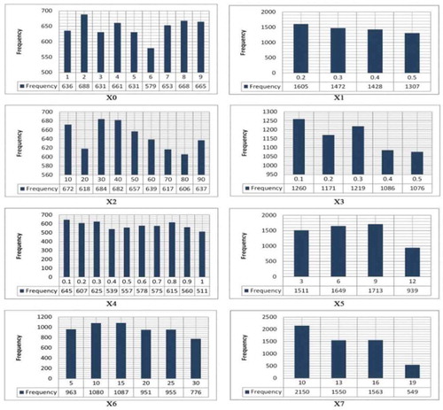
Table 2 presents an example of a dataset. There are four continuous variables (X1, X2, X3, and X4) and four discrete variables (X0, X5, X6, and X7) in this model. The domain of each variable is presented in Figure 4. The variables X5 (Month), X6 (Day), X7 (Hour), range respectively from 1 to 12, 1 to 30, and 7 to 19.

Table 2. Sample of dataset

X0	X1	X2	X3	X4	X5	X6	X7	Y
Number	Length(m)	Rotation(degree)	Distance(m)	Reflection(per cent)	Month	Day	hour	illuminance(lux)
3	0.31	47	0.2	0.56	1	21	14	2812.275
9	0.48	69	0.14	0.53	2	14	9	1434.667
3	0.28	11	0.04	0.17	8	17	14	664.3042
1	0.19	45	0.19	0.81	9	5	8	1313.013
9	0.18	67	0.09	0.5	4	29	16	303.8875
2	0.36	16	0.39	0.88	11	18	9	5391.842
9	0.45	66	0.09	0.29	2	13	8	484.4167
4	0.15	63	0.25	0.35	5	4	13	1669.971
2	0.49	57	0.22	0.18	8	10	12	1688.283
8	0.1	66	0.02	0.75	8	13	10	503.8667
6	0.24	82	0.07	0.38	2	1	10	2841.808
2	0.49	56	0.03	0.9	11	27	15	1346.2
6	0.12	42	0.44	0.82	1	1	13	5933.704
8	0.17	60	0.45	0.15	8	14	13	1788.779
6	0.22	56	0.36	0.68	2	6	9	2643.983
5	0.33	65	0.44	0.43	5	23	18	99.45
4	0.4	61	0.02	0.94	8	4	9	5558.421
8	0.33	81	0.14	0.32	2	24	10	961.2917
2	0.1	46	0.26	0.27	8	6	18	106.1125

Methods

This section provides a summary of data-driven statistical ideas and data assessment methods:

The first step in the majority of data analysis tools is to investigate the statistical characteristics of variables. The Spearman correlation coefficient can specify general monotonic relationships. This coefficient lies in the range of −1 to 1, where negative and positive signs indicate inverse and direct proportional relationships, respectively, and the magnitude reveals the strength of the relationship (Figure 6). Using the output variable, we illustrate the scatter diagram for each input variable (Figure 7). The empirical probability distributions of all input and output variables are shown in Figure 8. For the sake of simplicity, scatter diagrams often use standardized data (i.e., data in the range between −1 and 1) to facilitate comparison between measures that possibly show differences in the order of magnitude. Since the data used in this study are of non-Gaussian type, the Spearman correlation coefficient was used to statistically measure the intensity of each input and output variables.

Figure 6. Correlation matrix using Spearman rank correlations between the five input variables

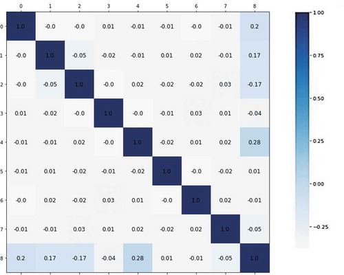
Figure 7. Scatter plot demonstrating visually the relationship between each standardize input variable and standardize output

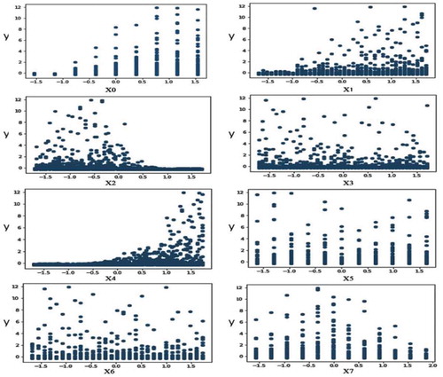
Figure 8. Probability density estimates using histograms of the five input variables, and the output variable

Mapping the input variables to the output variable

Given the number of samples (N = 5812) and input variables (M = 8), a compact matrix X€R^N×M was used that includes the available data:

This matrix typically has a response vector y €R N × 1 and thus we need to find the functional relationship between X and y; where y is illuminance and we have y = f(X). The function mapping tool is commonly called a learner in the machine learning literature. Given that the output variable spanned a continuous range of values, it seems necessary to use a regression technique. Nevertheless, in practice, it may be better to discretize the output variable to several categories and regard it as a classification problem. Recent studies demonstrate the potential of this concept, i.e. the discretization of a continuous-value output and the use of regression tools to find functional relationships. This section provides a brief overview of the AI models applied to this research. At the end of each method, the trained regression model is evaluated based on the test data and the R² metrics are computed. The dataset is divided into training (80%) and testing (20%) batches and is subjected to normalization pre-processing.

Polynomial Linear Regression

The polynomial regression is a form of regression analysis that models the relationship between the independent variable x and the dependent variable y, as an nth-degree polynomial in x (Zhou and Liu 2015). In the presence of a comprehensive database, the polynomial linear regression methods can produce reasonable results concerning the correlation between the model and the analyzed information, which applies to our situation. In developing a correlation method, it is needed to build a comprehensive dataset by conducting many parametric studies and then establish a simple equation using regression analysis. Due to the immense diversity of variables and cases, adequate simulations were conducted to generate a comprehensive dataset. A total number of 5812 simulations were run to have a high-accuracy model for future energy prediction.

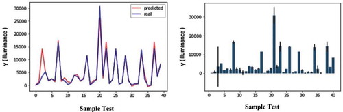
The polynomial degree in polynomial regression is a hyper-parameter fine-tuned based on trial and error. For this research, number 5 is the best-examined degree (Figure 9). This figure shows the results obtained from the polynomial linear regression with a degree of 5.

Figure 9. Error rate chart for comparison predicted and real values of sample test dataset (left), Bar chart with margin error rate for sample test dataset prediction(right) in polynomial linear regression model

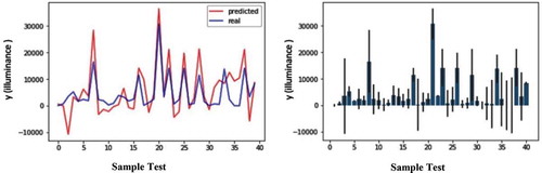
The right-hand image shows the bar chart with a margin error rate for the sample test prediction dataset. The left-hand image shows the error rate chart for comparison predicted and real values of the sample test dataset. In this method, the accuracy was estimated at 89%.

Random Forest Regression

The Classification and Regression Tree (CART) works via successive splitting of the input feature space into smaller and further smaller sub-regions. This procedure is like a tree that is divided into successively smaller branches, where each branch represents a sub-region of the input variable ranges. A natural expansion of CART, called Random forest (RF), is merely a set of many trees (Loh 2014; PS 2019). The training procedure is similar to CART, except that a subset of candidate variables, selected randomly, is used to pick optimal variables for each split. The practical results show the good performance of the RF algorithm in a wide range of areas.

In the present study, this characteristic is used to find the input variables with a powerful relationship with output variables. It is of note that the importance of each variable should not be assessed separately in this process; instead, they should be evaluated collectively for the feature subset used in the RF by using the ideas of relevance (the strength of association between variable and response), redundancy (the strength of association between variables), and complementarity (the strength of joint association between variables and response). This means that strongly correlated variables are redundant penalizing variables although they may be strongly correlated with the response (Breiman 2001).

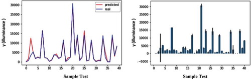
Figure 10 shows the results obtained from the random forest method. The right-hand image shows the bar chart with a margin error rate for the sample test prediction dataset. The left-hand image shows the error rate chart for comparing the predicted and real values of the sample test dataset. In this method, the accuracy was estimated at 96%.

Figure 10. Error rate chart for comparison predicted and real values of sample test dataset (left), Bar chart with margin error rate for sample test dataset prediction(right) in random forest model

Decision Tree

Decision Trees provide a non-parametric learning method for categorization and regression. In machine learning, the aim is to create a classification model (classification tree) capable of predicting the target variable value (also known as label or class) by learning simple decision rules (also known as attributes or predictors) extracted from data characteristics (Abdallah et al. 2018). Decision Trees are first suggested for information classification through a dividing-and-conquer approach that continues until the final leaf (Dougherty 2012). They are then applied in regression models with a huge number of factors and instances. Besides, their simplicity and effectiveness make them suitable for prediction.

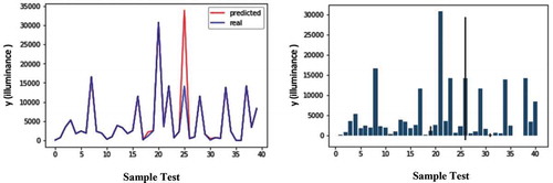
Figure 11 shows the results obtained from the Decision Tree method. The right-hand image presents the bar chart with a margin error rate for the sample test prediction dataset. The left-hand image shows the error rate chart for comparing the predicted and real values of the sample test dataset. In this method, the accuracy was estimated at 95%.

Figure 11. Error rate chart for comparison predicted and real values of sample test dataset (left), Bar chart with margin error rate for sample test dataset prediction(right) in decision tree model

Support Vector Regression (SVR)

The SVR method is commonly used for the analysis of classification and regression (Hu, Hu, and Du 2019). The goal is to find a function f(x, a) with a maximum deviation from the actual targets y_i observed for all training data. Moreover, this function should be as linear as SVR to be suitable for prediction purposes. Also, it is necessary to minimize the error rate by maximizing the hyperplane margin to differentiate between features (Henrique, Sobreiro, and Kimura 2018).

Figure 12 presents the results obtained from the SVR method. The right-hand image shows the bar chart with a margin error rate for the sample test prediction dataset. The left-hand image shows the error rate chart for comparing the predicted and real values of the sample test dataset. In this method, the accuracy was estimated at 46%.

Figure 12. Error rate chart for comparison predicted and real values of sample test dataset (left), Bar chart with margin error rate for sample test dataset prediction(right) in SVR model

Artificial Neural Network (ANN)

ANNs are powerful tools for estimating project parameters using current project conditions (Kim and Kim 2019b). ANNs, as a powerful experience-based learning and adapting method (Yadav and Chandel 2014), consist of four hidden layers. Each layer is comprised of n neurons or processing units, which are interconnected to all neurons in the neighbor layers. The first layer is called the input layer. In this study, the input layer has eight neurons, as the representative of independent variables. The input layer receives the data and feeds forward them throughout the network (Figure 13). The following hyper-parameters are used in this study: 4 hidden layers; Relu activation function; Adam optimizer; maximum epochs of 1000; and n neurons for each hidden layer (Figure 14); and MSE of the cost function.

Figure 13. Architecture of network

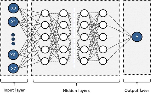
Figure 14. ANN model and number of neurons in each hidden layer

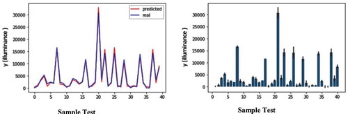
Figure 15 illustrates the results obtained from the ANN method. The right-hand image shows the bar chart with a margin error rate for the sample test prediction dataset. The left-hand image shows the error rate chart for comparison predicted and real values of the sample test dataset. In this method, the accuracy was estimated at 98%.

Figure 15. Error rate chart for comparison predicted and real values of sample test dataset (left), Bar chart with margin error rate for sample test dataset prediction(right) in ANN model

Conclusion and Discussion

This paper presents a parametric computational tool and method that can be used by architects and designers to generate, explore, evaluate, and predict the influence of various static external louvers on the internal measurement of illuminance. The method and tool were tested in a dataset that was created by simulation. The dataset showed the importance of generating and predicting data on results for various louvers. Such results allow the designer to have the ramifications of choosing variables of the louver that are optimal for internal illuminance. This study investigated the influence of the exterior louver design on interior energy performance as the AI model’s case study. The topic selected in the current study was a sample benchmark that can be generalized to other energy-related topics. The general methodology employed in this study can be extended to include more input variables in theory.

We developed a comprehensive structure to cover a greater variety of inputs for studying the illuminance. This study compared the accuracy of goal prediction using different methods, such as ANN, polynomial linear regression, RF, SVR, and DT. The models are based on regression metrics (i.e., MSE and R2 score). Analysis of the evaluation methods reveals that ANN produced higher and steadier results than RF, DT, and SVR. Also, it was found that ANN accurately estimates illuminance with a slight deviation from the ground truth. These findings are particularly convincing, given the accuracy of predictions. Moreover, they provide required variables in a short length of time without getting involved in simulation tools, such as Rhino. Furthermore, the proposed methodology can generate accurate values regardless of the simulation program. It is worth noting that illuminance values produced by Rhino are considered to reflect the valid values.

References

- Abdallah, I., V. Dertimanis, H. Mylonas, K. Tatsis, E. Chatzi, N. Dervilis, K. Worden, and E. Maguire. 2018. Fault diagnosis of wind turbine structures using decision tree learning algorithms with big data. Safety and Reliability–Safe Societies in a Changing World 3053–61.
- Aldawoud, A. 2013. Conventional fixed shading devices in comparison to an electrochromic glazing system in hot, dry climate. Energy and Buildings 59:104–10. doi:10.1016/j.enbuild.2012.12.031.
- Amasyali, K., and N. M. El-Gohary. 2018. A review of data-driven building energy consumption prediction studies. Renewable and Sustainable Energy Reviews 81:1192–205. doi:10.1016/j.rser.2017.04.095.
- Ayoub, M. 2020. A review on light transport algorithms and simulation tools to model daylighting inside buildings. Solar Energy 198:623–42. doi:10.1016/j.solener.2020.02.018.
- Breiman, L. 2001. Random forests. Machine Learning 45 (1):5–32. doi:10.1023/A:1010933404324.
- Choi, J., T. Lee, E. Ahn, and G. Piao. 2014. Parametric louver design system based on direct solar radiation control performance. Journal of Asian Architecture and Building Engineering 13 (1):57–62. doi:10.3130/jaabe.13.57.
- Choi, J., T.-K. Lee, E.-S. Ahn, G.-S. Piao, and J.-H. Lim. 2013. An evaluation system for parametric exterior louver designs including physical surroundings. Journal of the Architectural Institute of Korea Planning & Design 29 (10):91–98.
- Chou, J.-S., and D.-K. Bui. 2014. Modeling heating and cooling loads by artificial intelligence for energy-efficient building design. Energy and Buildings 82:437–46. doi:10.1016/j.enbuild.2014.07.036.
- Chou, J.-S., C.-W. Lin, A.-D. Pham, and J.-Y. Shao. 2015. Optimized artificial intelligence models for predicting project award price. Automation in Construction 54:106–15. doi:10.1016/j.autcon.2015.02.006.
- da Graça Carvalho, M. 2012. EU energy and climate change strategy. Energy 40 (1):19–22. doi:10.1016/j.energy.2012.01.012.
- Davoodi, A., P. Johansson, T. Laike, and M. Aries. 2019. Current use of lighting simulation tools in Sweden. In 60th International Conference of Scandinavian Simulation Society, SIMS 2019. Västerås, Sweden: Linköping University Electronic Press. August 13- 16.
- Dougherty, G. 2012. Pattern recognition and classification: An introduction. New York: Springer Science & Business Media.
- Fang, Y., and S. Cho. 2019. Design optimization of building geometry and fenestration for daylighting and energy performance. Solar Energy 191:7–18. doi:10.1016/j.solener.2019.08.039.
- Gill, A. S., J. D. Summers, and C. J. Turner. 2017. Comparing function structures and pruned function structures for market price prediction: An approach to benchmarking representation inferencing value. Ai Edam 31 (4):550–66.
- Grobman, Y. J., I. G. Capeluto, and G. Auster. 2016. External shading in buildings: Comparative analysis of daylighting performance in static and kinetic operation scenarios. Architectural Science Review.
- Henrique, B. M., V. A. Sobreiro, and H. Kimura. 2018. Stock price prediction using support vector regression on daily and up to the minute prices. The Journal of Finance and Data Science 4 (3):183–201. doi:10.1016/j.jfds.2018.04.003.
- Hu, Z., Z. Hu, and X. Du. 2019. One-class support vector machines with a bias constraint and its application in system reliability prediction. Artificial Intelligence for Engineering Design, Analysis and Manufacturing:Ai Edam 33 (3):346–358.
- Jakubiec, J. A., and C. F. Reinhart. 2011. Integrating daylight and thermal simulations using rhinoceros 3d, daysim and energyplus. In Proceedings of Building Simulation.
- Katsifaraki, A., B. Bueno, and T. E. Kuhn. 2017. A daylight optimized simulation-based shading controller for venetian blinds. Building and Environment 126:207–20. doi:10.1016/j.buildenv.2017.10.003.
- Khaled, J. M., N. S. Alharbi, S. Kadaikunnan, A. S. Alobaidi, M. N. Al-Anbr, K. Gopinath, A. Aurmugam, M. Govindarajan, and B. Giovanni. 2017. Green synthesis of ag nanoparticles with anti-bacterial activity using the leaf extract of an african medicinal plant, Ipomoea Asarifolia (Convolvulaceae). Journal of Cluster Science 28 (5):3009–19. doi:10.1007/s10876-017-1271-4.
- Khoroshiltseva, M., D. Slanzi, and I. Poli. 2016. A pareto-based multi-objective optimization algorithm to design energy-efficient shading devices. Applied Energy 184:1400–10. doi:10.1016/j.apenergy.2016.05.015.
- Kim, C.-H., and K.-S. Kim. 2019a. Development of sky luminance and daylight illuminance prediction methods for lighting energy saving in office buildings. Energies 12 (4):592. doi:10.3390/en12040592.
- Kim, G.-H., and S.-H. Kim. 2019b. Variable selection for artificial neural networks with applications for stock price prediction. Applied Artificial Intelligence 33 (1):54–67. doi:10.1080/08839514.2018.1525850.
- Kirimtat, A., B. K. Koyunbaba, I. Chatzikonstantinou, and S. Sariyildiz. 2016a. Review of simulation modeling for shading devices in buildings. Renewable and Sustainable Energy Reviews 53:23–49. doi:10.1016/j.rser.2015.08.020.
- Kirimtat, A., B. K. Koyunbaba, I. Chatzikonstantinou, S. Sariyildiz, and P. N. Suganthan. 2016b. Multi-Objective Optimization for Shading Devices in Buildings by Using Evolutionary Algorithms. In 2016 IEEE Congress on Evolutionary Computation (CEC), 3917–24. Vancouver, BC, Canada: IEEE.
- Kirimtat, A., O. Krejcar, B. Ekici, and M. Fatih Tasgetiren. 2019. Multi-objective energy and daylight optimization of amorphous shading devices in buildings. Solar Energy 185:100–11. doi:10.1016/j.solener.2019.04.048.
- Li, L., M. Qu, and S. Peng. 2016. Performance evaluation of building integrated solar thermal shading system: building energy consumption and daylight provision. Energy and Buildings 113:189–201. doi:10.1016/j.enbuild.2015.12.040.
- Loh, W.-Y. 2014. Classification and regression tree methods. Wiley StatsRef: Statistics Reference Online.
- Lorenz, C.-L., M. Packianather, A. B. Spaeth, and C. B. De Souza. 2018. Artificial Neural Network-Based Modelling for Daylight Evaluations. In Proceedings of the symposium on simulation for architecture and urban design, 2. Delft, The Netherlands: Society for Computer Simulation International.
- Machairas, V., A. Tsangrassoulis, and K. Axarli. 2014. Algorithms for optimization of building design: A review. Renewable and Sustainable Energy Reviews 31:101–12. doi:10.1016/j.rser.2013.11.036.
- Mahdavinejad, M., S. Matoor, N. Feyzmand, and A. Doroodgar. 2012. Horizontal distribution of illuminance with reference to Window Wall Ratio (Wwr) in office buildings in hot and dry climate, case of Iran, Tehran. In Applied mechanics and materials, ed. Prof. Xi Peng Xu, vol. 110, 72–76. Switzerland: Trans Tech Publisher.
- Manzan, M. 2014. Genetic optimization of external fixed shading devices. Energy and Buildings 72:431–40. doi:10.1016/j.enbuild.2014.01.007.
- Nasrollahi, N., and E. Shokri. 2016. Daylight illuminance in urban environments for visual comfort and energy performance. Renewable and Sustainable Energy Reviews 66:861–74. doi:10.1016/j.rser.2016.08.052.
- Nguyen, A.-T., S. Reiter, and P. Rigo. 2014. A review on simulation-based optimization methods applied to building performance analysis. Applied Energy 113:1043–58. doi:10.1016/j.apenergy.2013.08.061.
- PS, M. G. 2019. Performance evaluation of best feature subsets for crop yield prediction using machine learning algorithms. Applied Artificial Intelligence 33 (7):621–42. doi:10.1080/08839514.2019.1592343.
- Schardl, T. B. 2016. Performance engineering of multicore software: developing a science of fast code for the Post-Moore Era. Massachusetts, Cambridge: Doctoral dissertation, Massachusetts Institute of Technology.
- Skarning, G., C. Jensen, C. A. Hviid, and S. Svendsen. 2017. The effect of dynamic solar shading on energy, daylighting and thermal comfort in a nearly zero-energy loft room in Rome and Copenhagen. Energy and Buildings 135:302–11. doi:10.1016/j.enbuild.2016.11.053.
- Su, Z., and W. Yan. 2015. A fast genetic algorithm for solving architectural design optimization problems. Ai Edam 29 (4):457–69.
- Summers, J. D., C. Eckert, and A. K. Goel. 2017. Function in engineering: Benchmarking representations and models. Ai Edam 31 (4):401–12.
- Tregenza, P., and J. Mardaljevic. 2018. Daylighting buildings: Standards and the needs of the designer. Lighting Research & Technology 50 (1):63–79. doi:10.1177/1477153517740611.
- Tregenza, P. R. 2017. Uncertainty in daylight calculations. Lighting Research & Technology 49 (7):829–44. doi:10.1177/1477153516653786.
- Tzempelikos, A., and Y.-C. Chan. 2016. Estimating detailed optical properties of window shades from basic available data and modeling implications on daylighting and visual comfort. Energy and Buildings 126:396–407. doi:10.1016/j.enbuild.2016.05.038.
- Valladares-Rendón, L. G., G. Schmid, and S.-L. Lo. 2017. Review on energy savings by solar control techniques and optimal building orientation for the strategic placement of façade shading systems. Energy and Buildings 140:458–79. doi:10.1016/j.enbuild.2016.12.073.
- Wagdy, A., A. Sherif, H. Sabry, R. Arafa, and I. Mashaly. 2017. Daylighting simulation for the configuration of external sun-breakers on south oriented windows of hospital patient rooms under a clear desert sky. Solar Energy 149:164–75. doi:10.1016/j.solener.2017.04.009.
- Wan, K. K. W., D. H. W. Li, D. Liu, and J. C. Lam. 2011. Future trends of building heating and cooling loads and energy consumption in different climates. Building and Environment 46 (1):223–34. doi:10.1016/j.buildenv.2010.07.016.
- Weerasuriya, A. U. 2014. Predicting thermal performance of different roof systems by using decision tree method. Engineer 47 (3):27–37. doi:10.4038/engineer.v47i3.6892.
- Yadav, A. K., and S. S. Chandel. 2014. Solar radiation prediction using artificial neural network techniques: A review. Renewable and Sustainable Energy Reviews 33:772–81. doi:10.1016/j.rser.2013.08.055.
- Yao, J. 2014. An investigation into the impact of movable solar shades on energy, indoor thermal and visual comfort improvements. Building and Environment 71:24–32. doi:10.1016/j.buildenv.2013.09.011.
- Yun, G., D. Y. Park, and K. S. Kim. 2017. Appropriate activation threshold of the external blind for visual comfort and lighting energy saving in different climate conditions. Building and Environment 113:247–66. doi:10.1016/j.buildenv.2016.11.021.
- Zani, A., M. Andaloro, L. Deblasio, P. Ruttico, and A. G. Mainini. 2017. Computational design and parametric optimization approach with genetic algorithms of an innovative concrete shading device system. Procedia Engineering 180:1473–83. doi:10.1016/j.proeng.2017.04.310.
- Zhou, S., and D. Liu. 2015. Prediction of daylighting and energy performance using artificial neural network and support vector machine. Am. J. Civ. Eng. Archit 3 (3A):1–8.