A Collaborative Beetle Antennae Search Algorithm Using Memory Based Adaptive Learning

ABSTRACT

Recently developed Beetle Antennae Search algorithm (BAS) mimics the odor sensing mechanism of the longhorn beetles. The beetles have many species and many of these are advantageous to the nature as well as the mankind. Excepting the odor sensing activity, the beetles are naturally strong insects, and some of them have storage memory for adaptive learning and showcase social behavior. These natural mechanisms make them intelligent enough to perform the routine tasks for existence. This article proposes a novel Storage (Memory) Adaptive Collaborative BAS (SACBAS) algorithm, which incorporates the memory stored adaptive learning. This helps exploit the Group Extreme Value (GEV) instead of the Individual Extreme Values in swarm for faster convergence. Further, the SACBAS uses the reference points based on non-dominated sorting to diversify the state space. To test the data-driven performance of SACBAS, the Support Vector Machine (SVM) algorithm with linear kernel is used in this study. First, the SACBAS algorithm is tested on the multi-objective ZDT and DTLZ test-suites and compared with two recent techniques, the reference points based Non-dominated Sorting Genetic Algorithm (NSGA III) and Multi-Objective Evolutionary Algorithm based on Decomposition (MOEA/D). Second, the data-driven SACBAS is tested with real-world cases based on offline data. The proposed SACBAS is shown to handle the offline data efficiently and obtains promising results. The Friedman Test is carried out to differentiate the SACBAS from other two techniques and the Post Hoc Test confirms that the SACBAS obtains better HyperVolume indicator scores and outperforms the NSGA III and MOEA/D.

Introduction

The process of optimization is grounded on attaining the trade-off among several conflicting criteria for a given decision problem. In today’s world, every discipline of Science, Engineering, and Technology (SET) encounters such decision problems, which are characterized as computationally expensive problems. The main motive is to identify the viable trade-off points (solutions) with minimum computational effort. For such problems, Evolutionary Algorithms (EA) are identified as the ideal tools (Knowles and Nakayama 2008). The EAs are commonly classified as metaheuristic algorithms, which are being employed heavily in various Multi-Criteria Decision-Making (MCDM) problems of SET. These include building design and energy efficiency (Brownlee and Wright 2015; Delgarm et al. 2016), wireless sensory network design (Hacioglu et al. 2016; Murugeswari, Radhakrishnan, and Devaraj 2016), manufacturing system design (Azadeh et al. 2017; Dahane and Benyoucef 2016), parametric design of production processes (Li et al. 2016), software design, and analysis (Malhotra et al. 2018; Mkaouer et al. 2015), tuning and feature selection of machine learning techniques (Bouraoui, Jamoussi, and Ayed 2018; Geethanjali, Slochanal, and Bhavani 2008) etc.

Many metaheuristic algorithms are being evolved in the MCDM related literature, which include Multi-Objective Genetic Algorithm (MOGA) (Murata and Ishibuchi 1995), Non-dominated Sorting Genetic Algorithm II (NSGA II) (Deb et al. 2000), Multiple Objective Particle Swarm Optimization (MOPSO) (Coello and Lechuga 2002), Multi-Objective Evolutionary Algorithm based on Decomposition (MOEA/D) (Zhang and Li 2007), Archived Multi-objective Simulated Annealing (AMOSA) (Bandyopadhyay et al. 2008), Non-dominated Sorting Genetic Algorithm III (NSGA III) (Deb and Jain 2014). These techniques are iterative and aimed at attaining the trade-off points (also known as Pareto-optimal fronts) in the objective space with minimal computational effort.

Wolpert and Macready (1997) developed the theory of ‘no free lunch’ that explains the fact that it is not feasible to declare one optimization algorithm as most efficient for every problem being solved. The problem-specific knowledge or information is an important aid to the algorithmic design. That is the reason why it is harder to solve the black-box model (no information available about the problem) than the gray-box model (little information available about the problem). This theorem of optimization has inspired the experts to design many novel evolutionary and nature-inspired techniques in recent years. One such technique is the Beetle Antennae Search (BAS), which is a state-of-the-art metaheuristic algorithm developed based on the natural odor sensing activities of the longhorn beetles (Jiang and Li 2017). The BAS is a single solution-based search technique, which proceeds with the movement of a beetle depending upon the smell sensing using their long antennae. The BAS is a simple and fast algorithm, which does not consider any other complicated biological mechanisms apart from the smell or odor sensing activity. However, it is a proven fact that the beetles can manipulate their storage memory and learning skills while performing daily tasks for living (Alloway and Routtenberg 1967; Xue, Egas, and Yang 2007). Based on the above fact, the following contributions are made in this paper:

• It introduces the memory stored adaptive learning mechanism of beetles and proposes a multi-objective swarm-based collaborative BAS algorithm. The proposed algorithm is developed on the reference points-based non-dominated sorting technique (Deb and Jain 2014) with modified adaptive normalization and extended as a data-driven evolutionary optimization algorithm for the computationally expensive problems.

• The Collaborative BAS (SACBAS) is successfully tested on various published Multi-Objective test suites and the offline data-driven real-world cases collected from the literature. The overall performance of the SACBAS is compared with the NSGA III and MOEA/D.

• The algorithmic performances are analyzed using the Friedman test and the paired comparison test. The significant statistical differences among the algorithmic performances are portrayed and the proposed SACBAS is shown to obtain improvements over the NSGA III and MOEA/D.

The rest of this paper is structured as following, the literature review is presented in section 2; the proposed SACBAS algorithm is demonstrated in section 3; the computational results and an in-depth analysis are presented in section 4 and the concluding remarks are displayed in section 5.

Related Works

Recently computationally expensive optimization problems are trailing attention of many researchers, which demand many objective evaluations and consume higher CPU time. Such problems are being developed massively in the area of cross-disciplinary optimization (Shan and Wang 2010). The domain-specific mathematical functions must be derived as the objective functions for such problems, which is computationally expensive. However, alternative approach such as data-driven evolutionary optimization is evolving as the powerful methodology, which has become a state-of-the-art topic (Gröger, Niedermann, and Mitschang 2012). When the metaheuristic techniques are being used for the MCDM problems, the best practice is to employ the data-driven surrogate fitness functions. These are developed using existing Machine Learning (ML) functions. It often facilitates the use of traditional or existing optimization algorithms, such as the non-EA, EA. This type of optimization could also be classified as response surface optimization where only arbitrary set of input and output data samples are in hand (Simpson et al. 2008). This approach is highly capable of approximating the functional relationships among the sampled data obtained using Design of Experiment (DOE) techniques (An, Lu, and Cheng 2015). The exactness of the ML-based surrogate training would be an important issue for the data-driven meta-models. Therefore, the Mean Square Error (MSE), Root Mean Square Error (RMSE), Mean Absolute Error (MAE) could be used as the performance metrics. The lower value of the error indicates the higher accuracy of the model. Once the ML function is trained, an appropriate metaheuristic algorithm could be employed to find optimal set of solutions (Messac 2015). Data-driven evolutionary optimizers are quick and efficient; therefore, these are computationally inexpensive. The DOE techniques, such as the central composite design (CCD), Box-Behnken Design (BBD), D-Optimal Design (DOD), Latin Hypercube Sampling (LHS), Full Factorial Design (FFD), and Orthogonal Array Design (OAD) etc. could be employed to obtain the empirical sample points as the initial solution(s) to the metaheuristic algorithms. The DOE techniques usually enhance the design robustness for the process using the limited sample points (Giunta, Wojtkiewicz, and Eldred 2003).

Three types of surrogates/meta-models are available for the metaheuristic optimization algorithms, (1) global surrogate, (2) local surrogate, and (3) ensemble or combined surrogate (Sun et al. 2017). Global surrogate considers the absolute objective space, which causes more computational efforts. It is suitable for the low-dimensional or unconstrained problems. Therefore, this approach was suitable for the early studies (Sun et al. 2015). Haftka, Villanuev, and Chaudhuri (2016) published a detailed survey based on the global surrogate-based optimization. Recently the high-dimensional constrained problems are evolving with real-world data. The local surrogate modeling is being adopted for such problems. However, the local surrogates are intended to converge prematurely with the local optimal solutions. Krempser et al. (2017) depicts a similarity-driven additional local surrogate to enhance the performance of metaheuristic algorithm for structural optimization. A local distance-based surrogate is developed by Pilát and Neruda (2011), which is employed in a Memetic Algorithm (MA) and compared with other multi-objective EAs and global surrogate-assisted algorithms. It is often a good practice to use mixed forms of the global and local surrogates since the hybrid model can speed up with the small number of objective evaluations with exploration and exploitation (Wang et al. 2019). This hybrid model is known as ensemble surrogate. Tenne and Armfield (2009) proposes a MA framework with combined global and local surrogate for selection of the model based on the global and the local models. The trust-region approach and the RBF are used for the local surrogate. Zhou et al. (2007) combines the Gaussian Process-based global surrogate to the EA for population filtration and the RBF-based local surrogate to the Lamarckian evolution for fast convergence. The hybrid model consumes less CPU time.

Further, based on the type of data, the ML/surrogate-assisted metaheuristics could be classified as, (1) offline data-driven and (2) online data-driven techniques (Jin et al. 2018). The offline data-driven metaheuristics rely on the historical data, which implies that the new data are not available during the process of optimization. Therefore, the data quality and quantity, both are important factors for the offline data-driven metaheuristics (Wang et al. 2018). Whereas, online data-driven metaheuristics show more flexibilities since the new data could be added during the ML model training and optimization. It is thus said that the online methods are an extension or enhancement of the offline versions.

Recently various research on data-driven ML-Assisted optimization techniques are being works are being carried out by experts. Sun et al. (2015) developed a two-stage Particle Swarm Optimization (PSO) algorithm by incorporating a global and some local surrogate functions. The proposed technique is tested with some popular unimodal and multimodal problems from literature. Wang, Jin, and Jansen (2016) demonstrated the online and off-line based classifications of the ML-assisted EA techniques and developed an EA to optimize the offline data-driven trauma system. The CPU time is reduced using a multi-fidelity surrogate-management strategy. Haftka, Villanuev, and Chaudhuri (2016) performed a survey based on the surrogate-based global optimization with a focus on the balance between the exploration and exploitation search and Kriging-based models are reviewed primarily. Further, Sun et al. (2017) studied the combined effect of the ML-assisted PSO and a social learning PSO (SL-PSO) algorithm. SL-PSO worked on exploration and PSO worked on exploitation. The proposed method is successfully tested on the benchmark problems. Allmendinger et al. (2017) presented another survey and discussed the complexities in the ML-assisted multi-objective EAs. Authors found these complexities from the different real-world problems and analyzed them. This study pointed out multiple future scopes and demonstrated the applicability of the surrogate-assisted optimization in the industrial settings. Chugh et al. (2018) proposed a kriging-assisted reference vector guided EA (RVEA) and tested on some benchmark problems. Jin et al. (2018) considered five real-world cases of Blast Furnace Optimization, Trauma System Design Optimization, Optimization of Fused Magnesium Furnaces, Optimization of Airfoil Design, and Air Intake Ventilation System optimization where the ML-assisted EAs have shown promising solutions. Yu et al. (2018) developed a hierarchical combined algorithm based on PSO and SL-PSO, where the SL-PSO converges in the current search space for local optima and the PSO performs incremental search for global optima. The SL-PSO executes hierarchically within the scope of PSO and uses the RBF as fitness function. Pan et al. (2019) depicts a ML-assisted many-objective EA with the neural network, which approximates the correlation between target values and obtained values, i.e., training using the function-less data-driven model. The stated algorithm is shown to outperform the other EAs. Recently Chatterjee, Chakraborty, and Chowdhury (2019) surveyed various novel algorithms within the scope of robust design optimization and analyzed the performance of the ML models. Authors have picked up the best performing ML model and solved a large-size real-world problem.

It could be observed that the ML/surrogate-assisted metaheuristics are mostly based on the EAs such as genetic algorithm (GA), particle swarm optimization (PSO) etc. However, recently introduced EAs are believed to be competitive and capable of outperforming the earlier EAs (Sun et al. 2017, 2015). Many new metaheuristics have been proposed lately. These include the Cuckoo search (CS) (Gandomi, Yang, and Alavi 2013), Mine blast algorithm (MBA) (Sadollah et al. 2013), Krill Herd (KH) (Gandomi and Alavi 2012), Grey Wolf Optimization (GWO) (Mirjalili, Mirjalili, and Lewis 2014), African Buffalo Optimization (ABO) (Odili, Kahar, and Anwar 2015), Beetle Antennae Search (BAS) algorithm (Jiang and Li 2017), Ant-Lion Optimization (ALO) (Mirjalili 2015), which are yet to be explored for the data-driven optimization. Hence, there exists a missing link between the machine-learning and the optimization literature, which could help to evolve many new data-driven ML-assisted optimizers in coming days. This study aims to contribute to filling the abovementioned gap and introduce a novel data-driven evolutionary algorithm called the SACBAS algorithm. The SACBAS is developed using the memory stored adaptive learning and the reference points-based non-dominated sorting approach. The proposed technique is restricted to offline data-driven mode to improve the robustness of solution search and employed as a global-surrogate approach since the Group Extreme Value (GEV) based global search is solely considered in the SACBAS design. Since the SACBAS is developed using NSGA III framework, hence the algorithmic complexity is O(MN²) or O(N²log^M−2N) depending on the higher score (Deb and Jain 2014).

SACBAS Algorithm Framework

This paper introduces a data-driven storage adaptive collaborative BAS algorithm, which uses collaborative approach of the beetles using their memory stored adaptive learning and builds on the reference point-based non-dominated sorting concept (Deb and Jain 2014). The details of the BAS algorithm and the proposed extension are discussed in the following subsections.

Beetle Antennae Search Algorithm

The BAS algorithm is a recently proposed technique, which is inspired from the odor sensing mechanism of the beetles using their long antennae (Figure 1) (Jiang and Li 2017). The twin antennae work as the sensors with complex mechanism. Fundamental functions of such sensors are to follow the smell of the food and to sense the pheromone produced by the potential opposite gender for the reproduction. The Beetles can move their antennae 360° to sense the food or opposite genders. These movements are random in the neighborhood area and directed according to the concentration of odor. This implies that the beetles turn to the right or the left depending upon the higher concentration of the odor data gathered by the antennae sensor. Gradually, the step size between the previous position and the current position of the beetle reduces and the beetles move toward the most promising area of the search space. The initial version of the BAS algorithm is portrayed in Algorithm 1 (Wang and Chen 2018).

Figure 1. Antennae search mechanism with the storage memory operation: d_i is the distance between two antennae, δ_i is step length, (x_i, y_i) denotes the beetle position, X_GEVⁱ is the GEV of the i^thiteration, and f(x, y) is the fitness function (odor)

Algorithm 1: BAS

Input: Establish an objective function f(x^t), where

Variable x^t = [x₁, …, x_i]^T, initialize the

Parameters x⁰, d⁰, δ⁰.

Output: x_bst, f_bst.

Step 1: While (t < T_max) or (stopping condition) do

Step 2: Generate the direction vector unit $\vec{b}$ according to Eq. (3.1)

Step 3: Search in variable space with two kinds of antennae according to Eq. (3.2) or (3.3)

Step 4: Update the state variable x_t according to Eq. (3.4)

Step 5: if f(x_t) < f_bst then

Step 6: f_bst = f(x_t), x_bst = x_t

Step 7: End if

Step 8: Update sensing diameter d and step size δ using Eq. (3.5) and (3.6)

Step 9: End While

Step 10: Return x_bst, f_bst.

The BAS algorithm starts with a randomly generated position vector x^t at t^th time (t = 1, 2, …, T) and the position is evaluated using the fitness function f, which determines the smell or odor concentration (Zhu et al. 2018). The beetle decides the further move based on the smell concentration by generating the next promising position in the neighborhood of previous position using the exploration and exploitation. The directional move is determined by Eq. (3.1),

$\vec{b}=\frac{rnd\left(k,1\right)}{rnd\left(k,1\right)\parallel }\left(3.1\right)$

Where, rnd is a random function, and k is the dimension of the solution vector. The exploration is performed on the right (x_r) or the left (x_l) using Eq. (3.2) or Eq. (3.3),

$x_r=x^t+d^t\times \vec{b}\left(3.2\right)$

$x_l=x^t-d^t\times \vec{b}\left(3.3\right)$

Where d^t is the distance between the antennae at time t. Value of d^t must enfold the solution space. This guides the algorithm to escape from being stuck at local optima and improves the convergence speed. The next move is decided using the following rule,

$x^t=x^{t-1}+{\delta }^t\vec{b}sign\left(f\left(x_r\right)-f\left(x_l\right)\right)\left(3.4\right)$

Where δ^t is the step size at time t, which follows a decreasing function of t, and sign represents a sign function. The antennae distance d^t and the step size δ^t are updated using Eq. (3.5) and Eq. (3.6) respectively,

$d^t=0.95d^{t-1}+0.01\left(3.5\right)$

${\delta }^t=0.95{\delta }^{t-1}\left(3.6\right)$

Collaborative Multi-Objective BAS Algorithm

The original BAS algorithm is a developed as a single solution-based technique, which is similar to the Simulated Annealing (SA) algorithm. It starts with one random solution and iteratively improves it toward the global convergence. However, this version of the BAS is not suitable for the high-dimensional or multi-objective problems needing an initial population or swarm of initial solutions. To achieve that purpose, a collaborative form of BAS is developed in this paper. This collaborative BAS is completely different from the Beetle Swarm Optimization (BSO) developed using the PSO approach (Wang, Yang, and Liu 2018). Do the beetles share information with each other? Do they have significant velocity factors (like birds) to control their moves? These questions are not yet answered in literature. Therefore, the concept of BSO algorithm is not acceptable while describing the activities of the beetle swarm. The proposed collaborative BAS of this paper starts with a randomly generated N beetles (solutions) X = [X1, X2, …, Xn] walking collaboratively to the next positions. In the proposed technique, the agent beetles move individually in the swarm without passing information to each other. This phenomenon executes N single solution-based BAS in parallel. However, the beetles are assumed to have memories. Therefore, the beetles remember the GEV X_GEVⁱ⁻¹ for the swarm and learn using the learning factors c1 and c2 in every iteration of the algorithm. The GEV is the best beetle of the swarm which is the closest to the global optima.

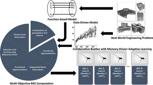
The multi-objective SACBAS is a surrogate-assisted collaborative BAS algorithm, which diversifies in the swarm using a set of reference points. These reference points are updated adaptively and distributed uniformly over the state space. In i^th iteration, the beetle swarm is denoted by swarm_i. With memory stored sequential movement operations (Figure 1), the new swarm is obtained as new_swarm_i. In the next step, the combined swarm is obtained using swarm_i = swarm_i U new_swarm_i. From the combined swarm, N number of best positions are selected with the non-dominated sorting and ranks. If the l^th ranked beetles are selected as the last level F_l in new swarm, then all the solutions from (l + 1)^th rank are discarded. If not all the solutions with l^th rank are selected, then only those solutions are selected, which could enhance the diversity. This selection procedure is accomplished using the generation of the reference points, the adaptive normalization of the swarm agents, the mapping of the swarm agents with the reference points, and niche-preservation procedure (Deb and Jain 2014). The proposed framework for the SACBAS is displayed in Figure 2.

Figure 2. The SACBAS Framework for data-driven optimization

Defining Reference Points

The reference points are obtained using a systematic procedure defined by ref. (Das and Dennis 1998), which distributes the reference points on a normalized hyper-plane. This hyper-plane is symmetrically inclined to the M number of the objective axes and defined using an (M-1)-dimensional unit simplex. The number of the reference points are decided on the number of divisions of each of the objective axes. Since the number of objectives considered in this study are not too many, therefore this technique provides good results. For P number of divisions, the number of reference points H would be computed using Eq. (3.7),

$H=C_P^{M+P-1}\left(3.7\right)$

For example, if M = 4, and P = 10, then the number of the reference points H = 286. Reference points could be expressed as an M × H dimensional matrix. It is assumed that the Pareto solutions are evenly dispersed over the Pareto front since the reference points are also scattered uniformly over hyper-plane. Z^ref denotes the set of the reference points and Z^ref = (z_k¹, z_k², …, z_k^H) ∀ k∈[1,H].

Adaptive Normalization of Swarm

The original adaptive normalization procedure proposed by (Deb and Jain 2014) solves a set of linear equation systems, which increase the computational complexity of the metaheuristic. For operational ease, the generalized normalization procedure is adopted in this paper. If Z_j^min = (z₁^min, z₂^min, …, z_M^min) denotes the set of ideal points consists of the minimum objective values for j^th member ∀ j∈[1, N] of the swarm. z_i^min is the i^th minimum objective value f_i ∀ i∈[1, M]. The z_i^max ∈Z^max is assumed to be the worst point for the i^th objective. Then, the normalized objective value fi*(x_j) is calculated using Eq. (3.8). The procedure is portrayed in Algorithm 2.

$f_i^{\ast }\left(x_j\right)=\frac{z_i^{max}-f_i\left(x_j\right)}{z_i^{max}-z_i^{min}}\mathrm{\forall }i\in \left[1,M\right]and\mathrm{\forall }j\in \left[1,N\right]\left(3.8\right)$

Algorithm 2: AdaptiveNormalization

Input: swarm, Z^max, Z^min

Output: Normalized Z^r

Step 1: z_i^min ← min f_i ∀ I ∈ [1, M]

Step 2: for j ←1 to N do

Step 3: for i←1 to M do

Step 4: if f_i (x_j) < z_i^min then

Step 5: z_i^min ← f_i (x_j)

Step 6: end

Step 7: end

Step 8: end

Step 9: for j ←1 to N do

Step 10: for i←1 to M do

Step 11: f_i*(x_j) ← (z_i^max − f_i (x_j))/(z_i^max − z_i^min)

Step 12: end

Step 13: end

Mapping of Swarm to Reference Points

On the normalized hyper-plane, the reference points are connected with the origin using the reference lines. Further, the perpendicular distance among the swarm members and reference lines are computed. For every reference point, the minimum perpendicular distance is obtained, and the corresponding member of swarm is mapped to that reference point. The procedure is portrayed in Algorithm 3,

Algorithm 3: Mapping

Input: Z^r, swarm

Output: τ (X ∈ swarm), d (X ∈ swarm) [τ is the nearest reference point and d is the distance from X to τ]

Step 1: for j ←1 to H do

Step 2: Calculate reference line w_j = z_j (z ∈ Z^r)

Step 3: end

Step 4: for j ←1 to N do

Step 5: for j ←1 to H do

Step 6: Calculate d^⊥(s, w) = || (s− w^Tsw/||w||²) ||

Step 7: end

Step 8: Assign τ(s) = w: argmin _{w ∈ Z}r d^⊥(s, w)

Step 9: Assign d(s) = d^⊥(s, τ(s))

Step 10: end

Niche-Preservation Procedure

Using this procedure, niches are tallied for every reference point based on the associated members of the swarm. Niche preservation is performed to select the desired candidates from F_l (the last selected level for the new swarm) using following rule. First, the reference points set is selected with minimum niche counts. If the number of such reference points are more than one, a random reference point is selected from above set. If the niche count is zero, the member is chosen based on the smallest perpendicular distance to the reference line else if the niche count is one or greater, a random member is selected from F_l front. Thereafter, the niche count is increased by one for the next iteration of the niche preservation procedure. If this selection operation is exhausted for a reference point, then that is excluded from the present iteration. This niche preservation procedure is repeated for the N – |pop| times (until the new swarm saturates). At the end of the procedure, the new swarm of size N is obtained.

Sequential Move Generation for BAS

In the collaborative multi-objective BAS framework, the position re-computation Eq. (3.4) is modified to include the domination characteristics of the solutions. Once the left and right positions are computed, the next step is to obtain the objective values for the right and left positions and select the next position based on the domination among these two and the x_GEVⁱ⁻¹. The individual extreme values are discarded to increase the convergence speed. This further simplifies the position reevaluation and eliminates the need for computing velocities (existent or non-existent?) of the beetles (Yang, Deb, and Fong 2011). The procedure is displayed in Algorithm 4.

Algorithm 4: SequentialMove

Input: x_r, x_l, f, x_GEVⁱ⁻¹, c1, c2

Output: x_i

Step 1: If x_l dominates x_r

Step 2: Compute x_i = (1-c2) × x_i + c1 × δ_i × $\vec{b}$ × x_GEVⁱ⁻¹

Step 3: Else If x_r dominates x_l

Step 4: Compute x_i = (1-c2) × x_i + c1 × δ_i × $\vec{b}$ × x_GEVⁱ⁻¹

Step 5: Else

Step 6: Compute x_i = x_GEVⁱ⁻¹

Step 7: End

Step 8: End

Step 9: Return x_i

Machine-Learning (ML) Fitness Functions

The objective evaluation is an important step for optimization algorithm. For the offline data-driven optimization problems, explicit mathematical objective functions are not readily available. Hence the ML fitness functions are suitable for such real-world problems (Chugh et al. 2018). In this study, four different ML functions are considered, and performances are compared for the offline data training. Depending on the performance measure scores, the best ML model is picked for the SACBAS algorithm. These function models are developed using the Decision Tree (DT), Support Vector Machine (SVM) based on linear and Gaussian kernels, and Radial Basis Function (RBF).

Decision Tree (DT)

A dataset of size n with output variable Y_i for i = 1, 2, …, k, (Y_i ∈ R) and decision variables X_j, j = 1, 2, …, p (x_j ∈ R^D) is considered. The DT model is trained in such a way that the values of Y could be predicted from the new X values. The Y variable holds ordered values and a DT regression model is fitted to each of the nodes of tree for the training. The DT model could be used for the high-dimensional data. The most popular DT approaches are AID (Morgan and Sonquist 1963) and the CART (Breiman et al. 1984) found in literature. Algorithm 5 displays the DT construction procedure,

Algorithm 5: DTConstruction

Step 1. Start the procedure at the root node or first node

Step 2. If stopping criteria is not met

Step 3. Compute two child nodes using the minimization of the sum of square error on nodes (S for each X) and split {X* ∈ S*} are obtained with the minimum overall X and S.

Step 4. Repeat step 3 for the child nodes

Step 5. End

DT models are also known as piecewise linear models since two separate linear models are required to fit on each of the node splits. Quinlan (1992) stated the formulation of S using the DT model in Eq. (3.9),

$S=\frac{m}{n}\left\{SD\left(t\right)-\frac{n_{L}SD\left(t_L\right)-n_{R}SD\left(t_R\right)}{n}\right\}\left(3.9\right)$

Where t is the node, n is the sample size, t_L and t_R are the node splits with sample size n_L and n_R, the SD is standard deviation, and m is the number of non-missing values in splits. Thereafter, multiple regression model is fitted to each of the nodes. Prediction error at t node is calculated using Eq. (3.10),

$Err\left(t\right)=\frac{{\sum }_i\left|Y_i-\widehat{Y_i}\right|}{n}\times \frac{n+v}{n-v}\left(3.10\right)$

Where v is the number of the parameters fitted in the model. Then, the number of regressors in each node is minimized using the backward stepwise regression. Tree pruning is performed using the bottom-up approach using the minimum prediction error check. Predicted values are smoothened using Eq. (3.11)

${\hat{y}}^{\ast \ast }=\frac{\left(n\hat{Y}+k{\hat{Y}}^{\ast }\right)}{\left(n+k\right)}\left(3.11\right)$

Where Y ̂** is smoothened predicted value, Y ̂* and Y ̂ are the predicted values at parent and child node, respectively, and k is a constant.

Support Vector Machines (SVM)

The SVM performs a data mapping from the low dimensional space to high dimensional space. In this approach, the input parameters X are mapped onto an m-dimensional attribute space using specific nonlinear mapping, which further converts it to a linear model in the same attribute space. The linear model is expressed as,

$f\left(X,\omega \right)=\sum _{j=1}^m{\omega }_j{g}_j\left(X\right)+\beta \left(3.12\right)$

Where g_j(X) (j = 1 … m) is non-linear transformation function and β is bias. The performance of regression is analyzed using the ε-insensitive loss function (Chapelle and Vapnik 2000),

$L\left(y,f\left(X,\omega \right)\right)=\left\{\begin{array}{c}0if\left|Y-f\left(X,\omega \right)\right|\le \epsilon \\ \left|Y-f\left(X,\omega \right)\right|-\epsilon Otherwise\end{array}\left(3.13\right)\right.$

The observed risk is defined using Eq. (3.14),

$R\left(\omega \right)=\frac{1}{n}\sum _{i=1}^{n}L\left(Y_i,d\left(X_i,\omega \right)\right)\left(3.14\right)$

The abovementioned regression model can be transformed into an optimization problem using Eq. (3.15),

$minZ=\frac{1}{2}{\omega }^2+C\sum _{k=1}^n\left({\gamma }_i+{\gamma }_i^{\ast }\right)\left(3.15\right)$

Subject to,

$\left\{\begin{array}{c}{Y}_i-f\left(X_i,\omega \right)\le \epsilon +{\gamma }_i^{\ast }\\ f\left(X_i,\omega \right)-Y_i\le \epsilon +{\gamma }_i\\ {\gamma }_i,{\gamma }_i^{\ast }\ge 0,i=1\dots n\end{array}\left(3.16\right)\right.$

Where γ_i and γ_i* (i = 1 … n) are positive slack variables, which can calculate the deviation of the input parameters beyond the ε-insensitive neighborhood. This optimization problem is known as primal, which could be transformed into a dual using Eq. (3.17),

$maxW\left(\alpha ,{\alpha }^{\ast }\right)=-\frac{1}{2}\sum _{i=1}^n\sum _{j=1}^n\left({\alpha }_i-{\alpha }_i^{\ast }\right)\left({\alpha }_j-{\alpha }_j^{\ast }\right)X_i,X_j+\sum _{i=1}^n\left({\alpha }_i-{\alpha }_i^{\ast }\right)Y_i+\sum _{i=1}^n\left({\alpha }_i-{\alpha }_i^{\ast }\right)\epsilon \left(3.17\right)$

Subject to,

$\sum _{i=1}^n\left({\alpha }_i-{\alpha }_i^{\ast }\right)=0,0\le {\alpha }_i,{\alpha }_i^{\ast }\le C,i=1,2,\dots ,n\left(3.18\right)$

The SVM fitting function is expressed as,

$f\left(X\right)=\sum _{i=1}^n\left({\alpha }_i-{\alpha }_i^{\ast }\right)K\left(X_i,X_j\right)+b\left(3.19\right)$

K(x_i, x_j) = <f(x_i),f(x_j)> is termed as the kernel function, which could be linear as well as non-linear (Gaussian) models.

Radial Basis Function (RBF)

The RBF is a popular function for fitting of the non-uniform data to predict responses. The RBF was first introduced by Hardy (1971). The RBF is demonstrated as an accurate method for predictive modeling of high-dimensional data (Arnaiz-González et al. 2016). The RBF is defined as f: R^D → R with Gaussian function of Eq. (3.20),

${\phi }_i\left(\vec{X}\right)=e^{-\frac{{\left|\left|\overrightarrow{X}-\overrightarrow{{\mu }_i}\right|\right|}^2}{2{\sigma }_i^2}}\left(3.20\right)$

The summation function is computed using Eq. (3.21),

$\mathrm{\varnothing }\left(\vec{X}\right)={\beta }^0+\sum _{i=1}^n{\omega }_i{e}^{-\frac{{\left|\left|\overrightarrow{X}-\overrightarrow{{\mu }_i}\right|\right|}^2}{2{\sigma }_i^2}}\left(3.21\right)$

Where n is the number of RBFs, µ is the midpoint of each RBF, X is input, σ > 0 is the Gaussian function, β⁰ is the bias, and ω is the weight of each RBF.

Initial Solution Generation for SACBAS

For the purpose of the initial solution generation, Latin Hypercube Sampling (LHS) is preferred, which is a popular method to sample the random solutions (Chen, Li, and Yao 2018; Wang et al. 2018). In this paper, a modified form of the LHS method is adopted, which generates the random sample (position of the beetle) uniformly within a specified range depending upon the actual range of the input variables. The algorithm 6 explains the modified LHS procedure. The proposed SACBAS algorithmic framework is portrayed in Algorithm 7.

Algorithm 6: ModifiedLHS

Input: No. of Sample points N (N = 1), Input Variables M with Lower Bound (LB) and Upper Bound (UB).

Output: Sample point in the form of solution string [X₁, X₂, …, X_M]

For i←1 >M do

1. Slope = UB-LB

2. Offset = LB

3. LUB = |UB|

4. SLOPE = J_N×LUB

5. OFFSET = J_N×LUB

6. SLOPE_i = J_N×1 ⊙ Slope_i and OFFSET_i = J_N×1 ⊙ offset_i for i ∈ [1, LUB]

7. X_NORM ← Basic LHS (N, LUB)

8. X_MOD ←SLOPE ⊙ X_NORM + OFFSET

End For

Return: X_MOD

Algorithm 7: SACBAS Pseudocode

%Parameter Initialization

Step 1: Number of Iterations (MaxIT), Size of Swarm (N), distance between antennae d⁰, step size δ⁰, learning factors (c1, c2), nondom = φ

%Functional Initialization

Step 2: →Z^ref = ReferencePointGenerator ()

Step 3: →Swarm⁰ = InitializeSwarm ()

Step 4: →Z^max = IdealPointGenerator ()

Step 5: →fitness⁰ = FitnessFunction (Swarm⁰) %FitnessFunction is SVM_LinearKernel for data driven SACBAS

Step 6: →[F₁, F₂, …, F_l, …’] = Non-dominated Sorting (Swarm⁰)

Step 7: →GEV = F₁(1)

%Main Loop

Step 8: For i←1: MaxIT

Step 9: For j←1: N

Step 10: x_j← Swarm⁰ (j)

Step 11: Generate $\vec{b}$, x_r, x_l using Eq. (3.1–3.3)

Step 12: x_j^new ← SequentialMove (x_j)

Step 13: f_j ← f (x_j^new)

Step 14: End For

Step 15: . Swarm⁰_new ← [x₁^new, x₂^new, …, x_N^new]; fitness ←[f₁, f₂, …, f_N]

Step 16: Swarm⁰ ← Swarm⁰_new ∪ Swarm⁰

Step 17: [F₁, F₂, …, F_l, …] = Non-dominated Sorting (Swarm⁰)

Step 18: While (nondom < N) do

Step 19: nondom ← nondom ∪ F_{k (k←k+1)}

Step 20: If last front included in nondom is F_l

Step 21: If Size(nondom) = = N then

Step 22: Swarm⁰ ← nondom;

Step 23: break

Step 24: Else Swarm⁰ ← F₁ + F₂ + … + F_l-1

Step 25: Z^r ← AdaptiveNormalization (Swarm⁰, Z^max, Z^min)

Step 26: [τ(x), d(x)] ← Mapping (Z^r, Swarm⁰) ∀x ∈ Swarm⁰

Step 27: Calculate the number of niche for reference points

Step 28: [N-Size(Swarm⁰) solutions] = NichePreservationProcedure(Swarm⁰, Z^r, τ, d, F_l)

Step 29: End If

Step 30: End If

Step 31: End While

Step 32: Update the antennae distance d and step size δ using Eq. (3.5) and (3.6)

Step 33: End For

Computational Studies

The proposed SACBAS is coded in the MATLAB on a 2.11 GHz Intel i7 computer. The proposed SACBAS is compared with other two latest metaheuristic algorithms, NSGA III (Deb and Jain 2014) and MOEA/D (Zhang and Li 2007). In the first place, the multi-objective form of the SACBAS is tested on the eleven benchmark test problems taken from ZDT (Zitzler, Deb, and Thiele 2000) and DTLZ (Deb et al. 2001) problem suites. For ZDT, the problem dimension is set as 20 for ZDT1, ZDT2, ZDT3, ZDT4, and ZDT6. For the DTLZ, the experiments are performed on the 3-objective and the 5-objective problems for DTLZ1, DTLZ2, DTLZ3, DTLZ4, DTLZ5, and DTLZ6. Then, in the second place, the data-driven SACBAS algorithm is validated using offline data, which are the Energy Efficiency (EE) for residential building data (Tsanasa and Xifara 2012), Closed Loop Engine (CLE) control data (Engine Timing Model with Closed Loop Control 1994), Concrete Slump (CS) data (Yeh 2007), and capital Stock Portfolio Performance (SPP) data (Liu and Yeh 2017). These real-world datasets could be directly accessible from the UCI Machine Learning (ML) repository (https://archive.ics.uci.edu/ml/index.php) and Mendeley data. The Hypervolume indicator (HV) is considered as the performance measure for the SACBAS, NSGA III, and MOEA/D algorithms (Augera et al. 2012). The HV calculates the volume area covered between the obtained Pareto frontier and the reference point on the objective space. According to ref. (Bringmann and Friedrich 2010) an optimization problem could be defined using some random dimension of decision variables X, where the objective is to minimize f(X): X → ℝ ^d_≥0. The d is the dimension of the problem. A probable solution point x belongs to the decision space X, which could be recognized with the corresponding fitness value in the solution space. If SWARM is the size of initial solution set, then the HV is computed using Eq. (4.1).

$HV\left(SWARM\right)=VOL\left(\underset{\left(x_1,x_2,\dots ,x_d\right)\in SWARM}{\cup }\left[0,x_1\right]\times \left[0,x_2\right]\times \dots \times \left[0,x_d\right]\right)\left(4.1\right)$

The VOL operation is performed using Lebesgue measure (Kestelman 1960). The higher is the HV indicator score, the better is the algorithmic performance.

Multi-Objective Performance Analysis on the ZDT and DTLZ Test Problems

The algorithms are executed for 15 trial runs for each of the test problems. The algorithmic parameters are obtained after rigorous testing and displayed in Table 1. For the selection of the parameters, the trade-off between the computational time and solution qualities are considered. For ZDT problems, the best (MAX) and worst (MIN) scores for HV indicator are obtained and presented in Table 2. Obtained Pareto fronts are portrayed in Figure 3- Figure 4Figure 5Figure 6Figure 7. The comparison among algorithmic performances is portrayed using boxplots in Figure 8. For ZDT3 and ZDT6, the SACBAS performs extremely well and obtains better HV scores than the NSGA III and MOEA/D. For ZDT1 and ZDT2, the mean HV scores obtained by all the three algorithms lie in the same region. Whereas, the SACBAS performs at per with the MOEA/D and better than the NSGA III for ZDT4. It could also be observed that the SACBAS obtains smaller number of Pareto solutions than the NSGA III and MOEA/D. However, the mean HV scores are better in most of the cases. This phenomenon proves the robustness and consistency of the SACBAS algorithm. If computational complexities are considered, the SACBAS has shown similar performance with the NSGA III. However, the MOEA/D performs faster than the SACBAS and NSGA III.

Table 1. Parameters for the SACBAS, NSGA III, and MOEA/D

SACBAS		NSGA III		MOEA/D
Swarm Size	100	Population Size	100	Population Size	100
Iteration No.	50	Generation No.	50	Generation No.	50
C1	0.2	PCrossover	0.5	Archive No.	100
C2	0.2	PMutation	0.02	PCrossover	0.5

Table 2. Comparison among SACBAS, NSGA III, and MOEA/D based on ZDT MOPs

				HyperVolume			CPU Time (S)
MOP	nVar	nObj	HV	SACBAS	NSGA III	MOEA/D	SACBAS	NSGA III	MOEA/D
ZDT1	20	2	MAX	5.41E-01	5.41E-01	5.46E-01	18.37	17.23	7.17
			MIN	4.53E-01	4.77E-01	4.65E-01
			MEAN	5.00E-01	5.00E-01	5.00E-01
ZDT2		2	MAX	5.45E-01	5.45E-01	5.57E-01	21.67	21.12	6.22
	20		MIN	4.67E-01	4.69E-01	4.64E-01
			MEAN	5.01E-01	4.99E-01	5.00E-01
ZDT3	20	2	MAX	5.27E-01	5.35E-01	5.47E-01	19.28	20.62	7.12
			MIN	4.65E-01	4.59E-01	4.60E-01
			MEAN	5.02E-01	4.98E-01	5.04E-01
ZDT4	20	2	MAX	5.30E-01	5.44E-01	5.30E-01	20.14	20.88	5.78
			MIN	4.64E-01	4.65E-01	4.74E-01
			MEAN	5.00E-01	4.98E-01	5.02E-01
ZDT6	20	2	MAX	5.28E-01	5.31E-01	5.36E-01	19.92	18.045	6.09
			MIN	4.55E-01	4.72E-01	4.59E-01
			MEAN	5.04E-01	4.99E-01	5.03E-01

Figure 3. ZDT1 Pareto Curves obtained using SACBAS, NSGA III, and MOEA/D

Figure 4. ZDT2 Pareto Curves obtained using SACBAS, NSGA III, and MOEA/D

Figure 5. ZDT3 Pareto Curves obtained using SACBAS, NSGA III, and MOEA/D

Figure 6. ZDT4 Pareto Curves obtained using SACBAS, NSGA III, and MOEA/D

Figure 7. ZDT6 Pareto Curves obtained using SACBAS, NSGA III, and MOEA/D

Figure 8. Comparison among SACBAS, NSGA III, and MOEA/D for ZDT problems using box plots

The justification could be that the goal of the development of MOEA/D is to reduce the computational complexities using decomposition method (Zhang and Li 2007). Whereas the SACBAS algorithm follows the trail of the NSGA III.

The SACBAS algorithm is further applied on the DTLZ test problems. The DTLZ problems are harder than the ZDT problems. Fig. 9, 11, 13, 15, 17, and 19 depict the Pareto fronts obtained by the SACBAS, NSGA III, and MOEA/D algorithms for 3-objective DTLZ problems. Fig. 10, 12, 14, 16, 18, and 20 portray the Pareto fronts for 5-objective DTLZ problems obtained by the SACBAS, NSGA III, and MOEA/D algorithms. The comparison among the algorithmic performances for 3-objective problems are portrayed using boxplots in Figure 21. It could be observed that the SACBAS performs very well for DTLZ1, DTLZ2, DTLZ4, DTLZ5 3-objective problems. Whereas, the NSGA III performs slightly better for the DTLZ3, and the MOEA/D performs superior for the DTLZ6 3-objective problem. Figure 22 shows the performance comparison among the three algorithms for the 5-objective DTLZ problems. The SACBAS shows improved HV scores for almost all the test problems except DTLZ6. The MOEA/D obtains slightly better mean HV scores for DTLZ6. Table 3 demonstrates the overall results for DTLZ test problems based on HV scores. Computational time scores are better for the MOEA/D algorithm than other two as expected.

Table 3. Comparison among SACBAS, NSGA III, and MOEA/D based on DTLZ MOPs

			HyperVolume Indicator				CPU Time (S)
MOP	nVar	nObj	Scores	SACBAS	NSGA III	MOEA/D	SACBAS	NSGA III	MOEA/D
DTLZ1	7	3	MAX	8.98E-01	8.79E-01	8.82E-01	22.6	25.7	15.53
			MIN	8.37E-01	6.52E-01	7.36E-01
			MEAN	8.69E-01	8.02E-01	7.93E-01
	9	5	MAX	7.31E-01	8.23E-01	6.33E-01	259.1	253.6	105.4
			MIN	6.34E-01	6.01E-01	5.14E-01
			MEAN	6.96E-01	6.94E-01	3.21E-01
DTLZ2	12	3	MAX	8.91E-01	8.92E-01	8.88E-01	23.46	25.34	15.6
			MIN	8.00E-01	6.72E-01	8.22E-01
			MEAN	8.63E-01	8.48E-01	8.56E-01
	14	5	MAX	8.34E-01	8.03E-01	7.71E-01	256.36	259.07	113.28
			MIN	6.24E-01	2.21E-01	4.82E-01
			MEAN	7.40E-01	5.04E-01	6.29E-01
DTLZ3	12	3	MAX	8.57E-01	8.92E-01	8.16E-01	24.29	25.27	12.98
			MIN	6.72E-01	7.92E-01	5.47E-01
			MEAN	8.05E-01	8.52E-01	6.78E-01
	14	5	MAX	8.01E-01	7.28E-01	6.60E-01	257.82	254.05	100.32
			MIN	5.65E-01	4.76E-01	3.63E-01
			MEAN	7.20E-01	5.95E-01	4.56E-01
DTLZ4	12	3	MAX	6.12E-01	8.22E-01	2.86E-01	23.86	25.78	14.57
			MIN	5.82E-01	5.16E-01	2.12E-01
			MEAN	5.47E-01	6.08E-01	2.51E-01
	14	5	MAX	3.02E-01	2.16E-01	2.57E-01	267.19	265.48	113.56
			MIN	1.79E-01	4.60E-02	5.10E-02
			MEAN	2.56E-01	8.79E-02	1.11E-01
DTLZ5	12	3	MAX	8.79E-01	8.07E-01	7.62E-01	25.97	27.8	17.14
			MIN	8.37E-01	6.86E-01	5.93E-01
			MEAN	7.80E-01	6.02E-01	6.54E-01
	14	5	MAX	6.52E-01	4.80E-01	5.61E-01	282.12	295.9	118.37
			MIN	3.84E-01	1.54E-01	2.85E-01
			MEAN	5.67E-01	2.82E-01	3.37E-01
DTLZ6	12	3	MAX	8.94E-01	8.94E-01	8.87E-01	28.23	28.17	17.25
			MIN	8.60E-01	8.17E-01	8.60E-01
			MEAN	8.17E-01	4.96E-01	8.13E-01
	14	5	MAX	8.15E-01	7.59E-01	7.38E-01	278.58	277.58	114.16
			MIN	5.68E-01	1.81E-01	6.20E-01
			MEAN	6.78E-01	4.34E-01	6.91E-01

Figure 9. DTLZ1 Pareto Curves for 3-Objective Problem by SACBAS, NSGA III, and MOEA/D

Figure 10. DTLZ1 Pareto Curves for 5-Objective Problem by SACBAS, NSGA III, and MOEA/D

Figure 11. DTLZ2 Pareto Curves for 3-Objective Problem by SACBAS, NSGA III, and MOEA/D

Figure 12. DTLZ2 Pareto Curves for 5-Objective Problem by SACBAS, NSGA III, and MOEA/D

Figure 13. DTLZ3 Pareto Curves for 3-Objective Problem by SACBAS, NSGA III, and MOEA/D

Figure 14. DTLZ3 Pareto Curves for 5-Objective Problem by SACBAS, NSGA III, and MOEA/D

Figure 15. DTLZ4 Pareto Curves for 3-Objective Problem by SACBAS, NSGA III, and MOEA/D

Figure 16. DTLZ4 Pareto Curves for 5-Objective Problem by SACBAS, NSGA III, and MOEA/D

Figure 17. DTLZ5 Pareto Curves for 3-Objective Problem by SACBAS, NSGA III, and MOEA/D

Figure 18. DTLZ5 Pareto Curves for 5-Objective Problem by SACBAS, NSGA III, and MOEA/D

Figure 19. DTLZ6 Pareto Curves for 3-Objective Problem by SACBAS, NSGA III, and MOEA/D

Figure 20. DTLZ6 Pareto Curves for 5-Objective Problem by SACBAS, NSGA III, and MOEA/D

Figure 21. Comparison among SACBAS, NSGA III, and MOEA/D for DTLZ 3-objective problems using box plots

Figure 22. Comparison among SACBAS, NSGA III, and MOEA/D for DTLZ 5-objective problems using box plots

Data-Driven Evolutionary Optimization Analysis on Offline Data

Four cases are considered from the literature, which are based on the real-world data. These are complicated multi-dimensional data with more than one objective to be considered (2–6). These cases are based on the offline data, which means that the experimentations or investigations are conducted before and the data are collected for analysis. Therefore, new data are not available during the optimization process. Due to the availability of the limited data or absence of new data, it is essential to obtain accurately trained ML-based surrogate models. For that matter, four different functions based on DT, SVM, and RBF are considered. The best function is selected based on the performances of these functions on all the case data. The HV indicator is also employed to measure the performance of the SACBAS algorithm with respect to the NSGA III and MOEA/D. The performance of the surrogate function is evaluated using Root Mean Square Error (RMSE) and Mean Absolute Error (MAE). The expressions of the RMSE and MAE are portrayed in Eq. (4.2) and Eq. (4.3) respectively.

$RMSE=\frac{1}{N}\sqrt{\sum _i{\left(Y_i-t_i\right)}^2}\left(4.2\right)$

$MAE=\frac{{\sum }_i|Y_i-t_i|}{N}\left(4.3\right)$

Where N is the number of observations, Y_i is the observed value for i^th observation and t_i is the i^th target value. The comparison study among the surrogate functions is displayed in Table 4. It could be observed that the SVM outperforms the DT and RBF functions. Among both SVMs, the SVM with linear kernel shows better RSME and MAE scores than the SVM with Gaussian kernel for the EE data, CLE data, and CS data. However, it obtains near best scores for SP data. Based on the analysis, the SVM with linear kernel is selected as the target function. All the three metaheuristic algorithms are applied on the selected SVM function. These algorithms performed well for all the four offline datasets. The obtained Pareto fronts are displayed in Fig. 23–26.

Table 4. Comparison among surrogate models based on RMSE and MAE scores

	nVar	nObj	Decision Tree		SVM (Linear Kernel)		SVM (Gaussian Kernel)		RBF
			RMSE	MAE	RMSE	MAE	RMSE	MAE	RMSE	MAE
EE Data	8	2	3.29E+00	2.84E+00	3.25E+00	2.48E+00	9.27E+00	8.22E+00	5.50E+00	4.30E+00
CLE Data	3	2	1.97E+03	1.44E+03	4.58E+01	3.11E+01	4.47E+02	2.92E+02	3.17E+02	2.04E+02
CS Data	7	3	2.45E+01	1.62E+01	1.23E+01	7.79E+00	1.40E+01	1.07E+01	1.47E+01	1.18E+01
SPP Data	6	6	6.70E-02	4.30E-02	4.90E-02	3.00E-02	4.10E-02	3.00E-02	6.00E-02	4.00E-02

Figure 23. Pareto Curves for EE data by SACBAS, NSGA III, and MOEA/D

Figure 24. Pareto Curves for CLE Data by SACBAS, NSGA III, and MOEA/D

Figure 25. Pareto Curves for CS data by SACBAS, NSGA III, and MOEA/D

Figure 26. Pareto Curves for SP data by SACBAS, NSGA III, and MOEA/D

The results are obtained based on HV indicator and displayed in Table 5 and the comparison using boxplots is depicted in Figure 27. It could be observed that the SACBAS performs uniformly and attains very good mean HV scores. It can outperform the established techniques such as NSGA III and MOEA/D for high-dimensional and multi-objective problems.

Table 5. Comparison among SACBAS, NSGA III, and MOEA/D based on DTLZ MOPs

					HyperVolume			CPU Time (S)
DATA	nVar	nObj	HV	SACBAS	NSGA III	MOEA/D	SACBAS	NSGA III	MOEA/D
EE Data	6	2	MAX	5.39E-01	5.43E-01	5.36E-01	30.13	26.47	15.97
			MIN	4.71E-01	4.64E-01	4.65E-01
			MEAN	5.02E-01	5.00E-01	5.02E-01
CLE Data	3	2	MAX	5.43E-01	5.27E-01	5.44E-01	24.66	18.94	12.06
			MIN	4.65E-01	4.69E-01	4.64E-01
			MEAN	5.02E-01	5.02E-01	5.01E-01
CS data	7	3	MAX	4.84E-01	4.92E-01	5.03E-01	27.93	19.32	13.27
			MIN	4.23E-01	4.19E-01	4.21E-01
			MEAN	4.55E-01	4.51E-01	4.55E-01
SPP Data	6	6	MAX	3.70E-02	3.20E-02	3.20E-02	96.46	96.65	43.99
			MIN	1.30E-02	1.30E-02	1.00E-02
			MEAN	2.30E-02	2.00E-02	2.10E-02

Figure 27. Comparison among SACBAS, NSGA III, and MOEA/D for all four offline data by box plots

Nonparametric Statistical Comparisons among the SACBAS, NSGA III, and MOEA/D

It is highly desirable to quantify the performance of a metaheuristic statistically. The numerical HV scores obtained from Table 2, 3, and 5 are close to each other. It is not an easy task to pick up the best performing metaheuristic with significant differences without statistical test. The nonparametric tests are suitable for such analyses where more than two metaheuristics are considered (Veillegas 2011). For that matter, Friedman rank test is applied on all the three algorithms. The test would confirm if at least one algorithm performs differently than others. All the test problem instances are considered in cumulative form for the statistical test. The HV scores are used for the test. The null hypothesis and alternative hypothesis are defined as,

H0: There is no significant difference among the metaheuristics (null hypothesis)

H1: At least one algorithm is different than others performance wise (alternative hypothesis)

In the first step of the Friedman rank test, the HV scores are ranked using R(HV_ij) where HV_ij is the HV score obtained by i^th algorithm for j^th problem. However, the ranks are assigned for a particular algorithm and the ranks obtained for an algorithm are not correlated with the ranks obtained by another algorithm. Thereafter, the summation of all the squared ranks is obtained using Eq. (4.4),

$A_2=\sum _{i=1}^n\sum _{j=1}^m{\left[R\left(H{V}_{ij}\right)\right]}^2\left(4.4\right)$

Where n is the number of algorithms and m is the number of problems. Further, the sum of the ranks for each algorithm is obtained and the square form of these summations are summed again using Eq. (4.4). $B_2=\frac{1}{m}\hspace{0.17em}\sum _{i=1}^n{\left[\sum _{j=1}^{m}R\left(H{V}_{ij}\right)\right]}^2\left(4.4\right)$

The test statistic is computed using Eq. (4.5),

$T_2=\frac{\left(m-1\right)\left[B_2-mn{\left(n+1\right)}^2/4\right]}{A_2-B_2}\left(4.5\right)$

At this stage, at the level of α significance F_{1-α, n-1, (n-1)(m-1)} is obtained from the F distribution table. If the test statistic T₂ is greater than F_{1-α, n-1, (n-1)(m-1)} then the null hypothesis is rejected. Here the k1 = n-1 and k2 = (n-1)(m-1) denote the degree of freedom values. Friedman test is carried out on the data obtained from Table 2, 3, and 5. Total 63 data points are considered and presented in Table 6. The ranks and square of the ranks are computed and displayed in Table 6. It also displays the sum of the ranks and the sum of the square of the ranks. Using Eq. (4.3) and Eq. (4.4) the values of A₂ = 833 and B₂ = 723.19 are computed. The test statistic is calculated as T₂ = 18.525 using Eq. (4.5). For α = 0.05, from F distribution table F_{1-α, n-1, (n-1)(m-1)} = F_{0.95, 2, 124} = 2.6. Since T₂ ˃ F, the null hypothesis is rejected. Hence, the Friedman test concludes that there exists at least one algorithm, which performs differently than the other two. At this point, a Post Hoc test is required, which would perform the pairwise comparison tests to identify the metaheuristic(s) behaving differently (Veillegas 2011). For that matter, the absolute difference between the sums of the ranks of the algorithms i and k are calculated and put in the conditional Eq. (4.6). If the condition holds, then i^th and k^th algorithms are claimed as different to each other.

$\left|\sum _{j=1}^{m}R\left(H{V}_{ij}\right)-\sum _{j=1}^{m}R\left(H{V}_{kj}\right)\right|>t_{1-\frac{\alpha }{2},\left(n-1\right)\left(m-1\right)}{\left[\frac{2n\left(A_2-B_2\right)}{\left(n-1\right)\left(m-1\right)}\right]}^{0.5}\left(4.6\right)$

Table 6. Calculation of ranks, sum of ranks, square of ranks, and sum of square of ranks

No.	SACBAS	R	R^2	NSGA III	R	R^2	MOEA/D	R	R^2
1	0.898	1	1	0.879	3	9	0.882	2	4
2	0.837	1	1	0.652	3	9	0.736	2	4
3	0.869	1	1	0.8015	2	4	0.793	3	9
4	0.731	2	4	0.823	1	1	0.633	3	9
5	0.634	1	1	0.601	2	4	0.514	3	9
6	0.696	1	1	0.694	2	4	0.321	3	9
7	0.891	2	4	0.892	1	1	0.888	3	9
8	0.8	2	4	0.672	3	9	0.822	1	1
9	0.863	1	1	0.848	3	9	0.856	2	4
10	0.834	1	1	0.803	2	4	0.771	3	9
11	0.624	1	1	0.221	3	9	0.482	2	4
12	0.74	1	1	0.504	3	9	0.629	2	4
13	0.857	2	4	0.892	1	1	0.816	3	9
14	0.672	2	4	0.792	1	1	0.547	3	9
15	0.805	2	4	0.852	1	1	0.678	3	9
16	0.801	1	1	0.728	2	4	0.66	3	9
17	0.565	1	1	0.476	2	4	0.363	3	9
18	0.72	1	1	0.595	2	4	0.456	3	9
19	0.612	2	4	0.822	1	1	0.286	3	9
20	0.582	1	1	0.516	2	4	0.212	3	9
21	0.547	2	4	0.608	1	1	0.251	3	9
22	0.302	1	1	0.216	3	9	0.257	2	4
23	0.179	1	1	0.046	3	9	0.051	2	4
24	0.256	1	1	0.0879	3	9	0.111	2	4
25	0.879	1	1	0.807	2	4	0.762	3	9
26	0.837	1	1	0.686	2	4	0.593	3	9
27	0.78	1	1	0.602	3	9	0.654	2	4
28	0.652	1	1	0.48	3	9	0.561	2	4
29	0.384	1	1	0.154	3	9	0.285	2	4
30	0.567	1	1	0.282	3	9	0.337	2	4
31	0.894	1	1	0.894	1	1	0.887	3	9
32	0.86	1	1	0.817	3	9	0.86	1	1
33	0.817	1	1	0.496	3	9	0.813	2	4
34	0.815	1	1	0.759	2	4	0.738	3	9
35	0.568	2	4	0.181	3	9	0.62	1	1
36	0.678	2	4	0.434	3	9	0.691	1	1
37	0.541	2	4	0.541	2	4	0.546	1	1
38	0.453	3	9	0.477	1	1	0.465	2	4
39	0.5	1	1	0.5	1	1	0.5	1	1
40	0.545	2	4	0.545	2	4	0.557	1	1
41	0.467	2	4	0.469	1	1	0.464	3	9
42	0.501	1	1	0.499	3	9	0.5	2	4
43	0.527	3	9	0.535	2	4	0.547	1	1
44	0.465	1	1	0.459	3	9	0.46	2	4
45	0.502	2	4	0.498	3	9	0.504	1	1
46	0.53	2	4	0.544	1	1	0.53	2	4
47	0.464	3	9	0.465	2	4	0.474	1	1
48	0.5	2	4	0.498	3	9	0.502	1	1
49	0.528	3	9	0.531	2	4	0.536	1	1
50	0.455	3	9	0.472	1	1	0.459	2	4
51	0.504	1	1	0.499	3	9	0.503	2	4
52	0.539	2	4	0.543	1	1	0.536	3	9
53	0.471	1	1	0.464	3	9	0.465	2	4
54	0.502	1	1	0.5	3	9	0.502	1	1
55	0.543	2	4	0.527	3	9	0.544	1	1
56	0.465	2	4	0.469	1	1	0.464	3	9
57	0.502	1	1	0.502	1	1	0.501	3	9
58	0.484	3	9	0.492	2	4	0.503	1	1
59	0.423	1	1	0.419	3	9	0.421	2	4
60	0.455	1	1	0.451	3	9	0.455	1	1
61	0.037	1	1	0.032	2	4	0.032	2	4
62	0.013	1	1	0.013	1	1	0.01	3	9
63	0.023	1	1	0.02	3	9	0.021	2	4
SUM		94	168		137	341		134	324

The value of t_{1-α/2, (n-1)(m-1)} is obtained from t distribution table with α significance level and (n-1)(m-1) degree of freedom. This calculates t_{1-α/2, (n-1)(m-1)} = t_{0.975, 124} = 1.96 and the right hand side of Eq. (4.6) becomes 1.96[2 n(A₂-B₂)/(n-1)(m-1)]^0.5 = 1.96×(111.58)°^.5 = 20.704. Further, the pairwise comparison matrix is obtained using the left-hand side of Eq. (4.6) and portrayed in Table 7. It could be observed that the SACBAS outperforms both the NSGA III and MOEA/D. Whereas the NSGA III and MOEA/D perform equally. Therefore, the SACBAS algorithm could be claimed as the superior among all.

Table 7. Pairwise comparison among algorithms

	NSBAS	NSGAIII	MOEAD
SACBAS		43	40
NSGA III	~		3
MOEAD	~	~

Conclusions

This paper presents a novel Storage Adaptive Collaborative Beetle Antennae Search algorithm (SACBAS), which could be applied on the mathematical function-based as well as the data-driven computational expensive problems. The SACBAS uses the memory stored adaptive learning-based sequential move and the reference point-based non-dominated sorting approach. The algorithm is developed using the Support Vector Machine (SVM) surrogate function as the SVM with linear kernel is shown to be superior to another SVM with Gaussian kernel, RBF, and decision tree-based models. Offline data are collected from the UCI ML repository and used for the model training. The proposed SACBAS is successfully compared with two other algorithms, the NSGA III and MOEA/D. The test suites utilized for the multi-objective performance comparison are based on the ZDT and DTLZ. A detailed Friedman test with Post Hoc analysis is carried out on the HyperVolume (HV) scores obtained by the algorithms and the proposed SACBAS is shown to outperform the NSGA III and MOEA/D. This article renders the following contributions,

• The proposed SACBAS is developed in such a way that it can execute parallel BAS algorithm modules for each of the swarm member. Therefore, each of the swarm members (beetle) can walk independently in the swarm.

• The beetles have information stored in memory and they use adaptive learning procedure to remember things. This phenomenon is incorporated in the SACBAS to memorize the group extreme value of the swarm and accelerate the convergence without the help of the individual extreme values for the swarm members.

• The reference point-based framework distributes the candidate solutions uniformly in the objective space. Further, the modified normalization procedure proposed in this study is suitable for high-dimensional data and reduces complexities. Both mechanisms are incorporated in the proposed SACBAS to obtain the Pareto optimal solutions for the high-dimensional problems with many objectives.

• The offline data-driven approach and global-surrogate is adopted in the proposed SACBAS algorithm for generalization, robustness, and prompt global optima.

The proposed SACBAS is in a process of further development. An attempt would be made to use it for more complex real-world many-objective problems such as manufacturing and production processes with combined form of the global and local surrogates for the online data.

Acknowledgments

This work is supported by the SFI Manufacturing (Project No. 237900) and funded by the Research Council of Norway (RCN).

Additional information

Funding

This work was supported by the Norges Forskningsråd [237900].

References

- Allmendinger, R., M. T. M. Emmerich, J. Hakanen, Y. Jin, and E. Rigoni. 2017. Surrogate‐assisted multicriteria optimization: Complexities, prospective solutions, and business case. Journal of Multi-Criteria Decision Analysis 24 (1–2):5–24. doi:10.1002/mcda.1605.
- Alloway, T. M., and A. Routtenberg. 1967. “Reminiscence” in the Cold Flour Beetle (Tenebrio molitor). Science 158 (3804):1066–67. doi:10.1126/science.158.3804.1066.
- An, Y., W. Lu, and W. Cheng. 2015. Surrogate Model Application to the Identification of Optimal Groundwater Exploitation Scheme Based on Regression Kriging Method—A Case Study of Western Jilin Province. International Journal of Environmental Research and Public Health 12 (8):8897–918. doi:10.3390/ijerph120808897.
- Arnaiz-González, Á., A. Fernández-Valdivielso, A. Bustillo, L. Norberto, and L. De Lacalle. 2016. Using artificial neural networks for the prediction of dimensional error on inclined surfaces manufactured by ball-end milling. The International Journal of Advanced Manufacturing Technology 83 (5–8):847–59. doi:10.1007/s00170-015-7543-y.
- Augera, A., J. Bader, D. Brockhoff, and E. Zitzler. 2012. Hypervolume-based multiobjective optimization: Theoretical foundations and practical implications. Theoretical Computer Science 425:75–103. doi:10.1016/j.tcs.2011.03.012.
- Azadeh, A., M. Ravanbakhsh, M. Rezaei-Malek, M. Sheikhalishahi, and A. Taheri-Moghaddam. 2017. Unique NSGA-II and MOPSO algorithms for improved dynamic cellular manufacturing systems considering human factors. Applied Mathematical Modelling 48:655–72. doi:10.1016/j.apm.2017.02.026.
- Bandyopadhyay, S., S. Saha, U. Maulik, and K. Deb. 2008. A Simulated Annealing-Based Multiobjective Optimization Algorithm: AMOSA. IEEE Transactions on Evolutionary Computation 12 (3):269–83. doi:10.1109/TEVC.2007.900837.
- Bouraoui, A., S. Jamoussi, and Y. B. Ayed. 2018. A multi-objective genetic algorithm for simultaneous model and feature selection for support vector machines. Artificial Intelligent Review 50 (2):261–81. doi:10.1007/s10462-017-9543-9.
- Breiman, L., J. H. Friedman, R. A. Olshen, and C. J. Stone. 1984. Chapman & Hall/CRC. Classification and Regression Trees, 368. https://doi.org/10.1201/9781315139470
- Bringmann, K., and T. Friedrich. 2010. An Efficient Algorithm for Computing Hypervolume Contributions. Evolutionary Computation 18 (3):383–402. doi:10.1162/EVCO_a_00012.
- Brownlee, A. E. I., and J. A. Wright. 2015. Constrained, mixed-integer and multi-objective optimisation of building designs by NSGA-II with fitness approximation. Applied Soft Computing 33:114–26. doi:10.1016/j.asoc.2015.04.010.
- Chapelle, O., and V. Vapnik. 2000. Model Selection for Support Vector Machines. NIPS’99 Proceedings of the 12th International Conference on Neural Information Processing Systems. Denver, CO: MIT Press Cambridge, MA, USA. 230–36. http://olivier.chapelle.cc/pub/nips99.pdf.
- Chatterjee, T., S. Chakraborty, and R. Chowdhury. 2019. A Critical Review of Surrogate Assisted Robust Design Optimization. Archives of Computational Methods in Engineering 26 (1):245–74. doi:10.1007/s11831-017-9240-5.
- Chen, R., K. Li, and X. Yao. 2018. Dynamic Multiobjectives Optimization With a Changing Number of Objectives. IEEE Transactions on Evolutionary Computation 22 (1):157–71. doi:10.1109/TEVC.2017.2669638.
- Chugh, T., Y. Jin, K. Miettinen, J. Hakanen, and K. Sindhya. 2018. A Surrogate-Assisted Reference Vector Guided Evolutionary Algorithm for Computationally Expensive Many-Objective Optimization. IEEE Transactions on Evolutionary Computation 22 (1):129–42. doi:10.1109/TEVC.2016.2622301.
- Coello, C. A. C., and M. S. Lechuga. 2002. MOPSO: A proposal for multiple objective particle swarm optimization. Proceedings of the 2002 Congress on Evolutionary Computation. CEC’02 (Cat. No.02TH8600). Honolulu, HI, USA: IEEE. 1051–56. 10.1109/CEC.2002.1004388.
- Dahane, M., and L. Benyoucef. 2016. An Adapted NSGA-II Algorithm for a Reconfigurable Manufacturing System (RMS) Design Under Machines Reliability Constraints. In Metaheuristics for Production Systems, ed. E. G. Talbi, F. Yalaoui, and L. Amodeo, vol. 60, 109–30. Switzerland: Springer. Operations Research/Computer Science Interfaces Series. doi:10.1007/978-3-319-23350-5_5.
- Das, I., and J. E. Dennis. 1998. Normal-Boundary Intersection: A New Method for Generating the Pareto Surface in Nonlinear Multicriteria Optimization Problems. SIAM Journal on Optimization 8 (3):631–57. doi:10.1137/S1052623496307510.
- Deb, K., S. Agrawal, A. Pratap, and T. Meyarivan. 2000. A Fast Elitist Non-dominated Sorting Genetic Algorithm for Multi-objective Optimization: NSGA-II. In Parallel Problem Solving from Nature PPSN VI. PPSN. Berlin, Heidelberg: Lecture Notes in Computer Scienceed., M. Schoenauer, K. Deb, G. Rudolph, X. Yao, E. Lutton, J. J. Merelo, and H. P. Schwefel, 849–58. Berlin, Heidelberg: Springer. 2000. 10.1007/3-540-45356-3_83.
- Deb, K., and H. Jain. 2014. An Evolutionary Many-Objective Optimization Algorithm Using Reference-Point-Based Nondominated Sorting Approach, Part I: Solving Problems With Box Constraints. IEEE Transactions on Evolutionary Computation 18 (4):577–601. doi:10.1109/TEVC.2013.2281535.
- Deb, K., L. Thiele, M. Laumanns, and E. Zitzler. 2001. Scalable test problems for evolutionary multi-objective optimization. Computer Engineering and Networks Laboratory (TIK), Swiss Federal Institute of Technology (ETH) doi:10.3929/ethz-a-004284199.
- Delgarm, N., B. Sajadi, S. Delgarm, and F. Kowsary. 2016. A novel approach for the simulation-based optimization of the buildings energy consumption using NSGA-II: Case study in Iran. Energy and Buildings 127:552–60. doi:10.1016/j.enbuild.2016.05.052.
- Engine Timing Model with Closed Loop Control. 1994. https://se.mathworks.com/help/simulink/slref/engine-timing-model-with-closed-loop-control.html.
- Gandomi, A. H., and A. H. Alavi. 2012. Krill herd: A new bio-inspired optimization algorithm. Communications in Nonlinear Science & Numerical Simulation 17 (12):4831–45. doi:10.1016/j.cnsns.2012.05.010.
- Gandomi, A. H., X. S. Yang, and A. H. Alavi. 2013. Cuckoo search algorithm: A metaheuristic approach to solve structural optimization problems. Engineering with Computers 29 (1):17–35. doi:10.1007/s00366-011-0241-y.
- Geethanjali, M., S. M. R. Slochanal, and R. Bhavani. 2008. PSO trained ANN-based differential protection scheme for power transformers. Neurocomputing 71 (4–6):4–6. doi:10.1016/j.neucom.2007.02.014.
- Giunta, A., S. Wojtkiewicz, and M. Eldred. 2003. Overview of Modern Design of Experiments Methods for Computational Simulations. Reno, Nevada, USA.: 41st Aerospace Sciences Meeting and Exhibit, Aerospace Sciences Meetings.
- Gröger, C., F. Niedermann, and B. Mitschang. 2012. Data Mining-driven Manufacturing Process Optimization. London, UK: Proceedings of the World Congress on Engineering. http://www.iaeng.org/publication/WCE2012/WCE2012_pp1475-1481.pdf.
- Hacioglu, G., V. Faryad, A. Kand, and E. Sesli. 2016. Multi objective clustering for wireless sensor networks. Expert Systems with Applications 59:86–100. doi:10.1016/j.eswa.2016.04.016.
- Haftka, R. T., D. Villanuev, and A. Chaudhuri. 2016. Parallel surrogate-assisted global optimization with expensive functions – A survey. Structural and Multidisciplinary Optimization 54 (1):3–13. doi:10.1007/s00158-016-1432-3.
- Hardy, R. L. 1971. Multiquadric equations of topography and other irregular surfaces. Journal of Geophysical Research 76 (8):1905/1915. doi:10.1029/JB076i008p01905.
- Jiang, X., and S. Li. 2017. BAS: Beetle Antennae Search Algorithm for Optimization Problems. arXiv:1710.10724 [cs.NE]. https://arxiv.org/pdf/1710.10724.pdf.
- Jin, Y., H. Wang, T. Chugh, D. Guo, and K. Miettinen. 2018. Data-Driven Evolutionary Optimization: An Overview and Case Studies. IEEE Transactions on Evolutionary Computation. doi:10.1109/TEVC.2018.2869001.
- Kestelman, H. 1960. Lebesgue Measure. Chap. 3 in Modern Theories of Integration, 67–91. New York: Dover.
- Knowles, J., and H. Nakayama. 2008. Meta-Modeling in Multiobjective Optimization. In Multiobjective Optimization, ed. J. Branke, K. Deb, K. Miettinen, and R. Słowiński, vol. 5252, 245–84. Springer, Berlin, Heidelberg. Lecture Notes in Computer Science. doi:10.1007/978-3-540-88908-3_10.
- Krempser, E., H. S. Bernardino, H. J. C. Barbosa, and A. C. C. Lemonge. 2017. Performance evaluation of local surrogate models in differential evolution-based optimum design of truss structures. Engineering Computations 34 (2):499–547. doi:10.1108/EC-06-2015-0176.
- Li, C., Q. Xiao, Y. Tang, and L. Li. 2016. A method integrating Taguchi, RSM and MOPSO to CNC machining parameters optimization for energy saving. Journal of Cleaner Production 135 (1):263–75. doi:10.1016/j.jclepro.2016.06.097.
- Liu, Y. C., and I. C. Yeh. 2017. Using mixture design and neural networks to build stock selection decision support systems. Neural Computing & Applications 28 (3):521–35. doi:10.1007/s00521-015-2090-x.
- Malhotra, R., S. Aggarwal, R. Girdhar, and R. Chugh. 2018. Bug localization in software using NSGA-II. 2018 IEEE Symposium on Computer Applications & Industrial Electronics (ISCAIE). Penang, Malaysia: IEEE. 10.1109/ISCAIE.2018.8405511.
- Messac, A. 2015. Optimization in Practice with MATLAB. NY, USA: Cambridge University Press. doi:10.1017/CBO9781316271391.
- Mirjalili, S. 2015. The Ant Lion Optimizer. Advances in Engineering Software 83:80–98. doi:10.1016/j.advengsoft.2015.01.010.
- Mirjalili, S., S. M. Mirjalili, and A. Lewis. 2014. Grey Wolf Optimizer. Advances in Engineering Software 69:46–61. doi:10.1016/j.advengsoft.2013.12.007.
- Mkaouer, W., M. Kessentini, A. Shaout, P. Koligheu, S. Bechikh, K. Deb, and A. Ouni. 2015. Many-Objective Software Remodularization Using NSGA-III. ACM Transactions on Software Engineering and Methodology 17: 1–17: 45 24(3):. doi:10.1145/2729974.
- Morgan, J. N., and J. A. Sonquist. 1963. Problems in the Analysis of Survey Data, and a Proposal. Journal of the American Statistical Association 58 (302):415–34. doi:10.2307/2283276.
- Murata, T., and H. Ishibuchi. 1995. MOGA: Multi-Objective Genetic Algorithms. Proceedings of 1995 IEEE International Conference on Evolutionary Computation. Perth, Australia. 289–94. http://www.academia.edu/download/43575182/MOGA_1995_Murata.pdf.
- Murugeswari, R., S. Radhakrishnan, and D. Devaraj. 2016. A multi-objective evolutionary algorithm based QoS routing in wireless mesh networks. Applied Soft Computing 40:517–25. doi:10.1016/j.asoc.2015.12.007.
- Odili, J. B., M. N. M. Kahar, and S. Anwar. 2015. African Buffalo Optimization: A Swarm-Intelligence Technique. Procedia Computer Science 76:443–48. doi:10.1016/j.procs.2015.12.291.
- Pan, L., C. He, Y. Tian, H. Wang, X. Zhang, and Y. Jin. 2019. A Classification-Based Surrogate-Assisted Evolutionary Algorithm for Expensive Many-Objective Optimization. IEEE Transactions on Evolutionary Computation 23 (1):74–88. doi:10.1109/TEVC.2018.2802784.
- Pilát, M., and R. Neruda. 2011. LAMM-MMA: Multiobjective memetic algorithm with local aggregate meta-model. GECCO ‘11 Proceedings of the 13th annual conference companion on Genetic and evolutionary computation. Dublin, Ireland. 10.1145/2001858.2001905.
- Quinlan, J. R. 1992. Learning with continuous classes. 5th Australian Joint Conference on Artificial Intelligence. Sydney, Australia. 343–48. https://sci2s.ugr.es/keel/pdf/algorithm/congreso/1992-Quinlan-AI.pdf.
- Sadollah, A., A. Bahreininejad, H. Eskandar, and M. Hamdi. 2013. Mine blast algorithm: A new population based algorithm for solving constrained engineering optimization problems. Applied Soft Computing 13 (5):2592–612. doi:10.1016/j.asoc.2012.11.026.
- Shan, S., and G. G. Wang. 2010. Survey of modeling and optimization strategies to solve high-dimensional design problems with computationally-expensive black-box functions. Structural and Multidisciplinary Optimization 41 (2):219–41. doi:10.1007/s00158-009-0420-2.
- Simpson, T., V. Toropov, V. Balabanov, and F. Viana. 2008. Design and Analysis of Computer Experiments in Multidisciplinary Design Optimization: A Review of How Far We Have Come - Or Not. British Columbia: 12th AIAA/ISSMO Multidisciplinary Analysis and Optimization Conference, Multidisciplinary Analysis Optimization Conferences, British Columbia, Canada.
- Sun, C., Y. Jin, R. Cheng, J. Ding, and J. Zeng. 2017. Surrogate-Assisted Cooperative Swarm Optimization of High-Dimensional Expensive Problems. IEEE Transactions on Evolutionary Computation 21 (4):644–60. doi:10.1109/TEVC.2017.2675628.
- Sun, C., Y. Jin, J. Zeng, and Y. Yu. 2015. A two-layer surrogate-assisted particle swarm optimization algorithm. Soft Computing 19 (6):1461–75. doi:10.1007/s00500-014-1283-z.
- Tenne, Y., and S. W. Armfield. 2009. A framework for memetic optimization using variable global and local surrogate models. Soft Computing 13 (8–9):781–92. doi:10.1007/s00500-008-0348-2.
- Tsanasa, A., and A. Xifara. 2012. Accurate quantitative estimation of energy performance of residential buildings using statistical machine learning tools. Energy and Buildings 49:560–67. doi:10.1016/j.enbuild.2012.03.003.
- Veillegas, J. G. 2011. use nonparametric tests to compare the performance of metaheuristic. http://or-labsticc.univ-ubs.fr/sites/default/files/Friedman%20test%20-24062011_0.pdf.
- Wang, H., Y. Jin, and J. O. Jansen. 2016. Data-Driven Surrogate-Assisted Multiobjective Evolutionary Optimization of a Trauma System. IEEE Transactions on Evolutionary Computation 20 (6):939–52. doi:10.1109/TEVC.2016.2555315.
- Wang, H., Y. Jin, C. Sun, and J. Doherty. 2018. Offline Data-Driven Evolutionary Optimization Using Selective Surrogate Ensembles. IEEE Transactions on Evolutionary Computation. doi:10.1109/TEVC.2018.2834881.
- Wang, J., and H. Chen. 2018. BSAS: Beetle Swarm Antennae Search Algorithm for Optimization Problems. arXiv:1807.10470 [cs.NE]. https://arxiv.org/pdf/1807.10470.pdf.
- Wang, T., L. Yang, and Q. Liu. 2018. Beetle Swarm Optimization Algorithm: Theory and Application. arXiv:1808.00206 [cs.NE]. https://arxiv.org/ftp/arxiv/papers/1808/1808.00206.pdf.
- Wang, Y., D. Q. Yin, S. Yang, and G. Sun. 2019. Global and Local Surrogate-Assisted Differential Evolution for Expensive Constrained Optimization Problems With Inequality Constraints. IEEE Transactions on Cybernetics 49 (5):1642–56. doi:10.1109/TCYB.2018.2809430.
- Wolpert, D. H., and W. G. Macready. 1997. No free lunch theorems for optimization. IEEE Transactions on Evolutionary Computation 1 (1):67–82. doi:10.1109/4235.585893.
- Xue, H. J., M. Egas, and X. K. Yang. 2007. Development of a positive preference–performance relationship in an oligophagous beetle: Adaptive learning? Entomologia Experimentalis Et Applicata 125 (2):119–24. doi:10.1111/j.1570-7458.2007.00605.x.
- Yang, X. S., S. Deb, and S. Fong. 2011. Accelerated Particle Swarm Optimization and Support Vector Machine for Business Optimization and Applications. In Networked Digital Technologies, ed. S. Fong, vol. 136, 53–66. Berlin, Heidelberg: Springer. doi:10.1007/978-3-642-22185-9_6.
- Yeh, I. C. 2007. Modeling slump flow of concrete using second-order regressions and artificial neural networks. Cement & Concrete Composites 29 (6):474–80. doi:10.1016/j.cemconcomp.2007.02.001.
- Yu, H., Y. Tan, J. Zeng, C. Sun, and Y. Jin. 2018. Surrogate-assisted hierarchical particle swarm optimization. Information Sciences 454-455:59–72. doi:10.1016/j.ins.2018.04.062.
- Zhang, Q., and H. Li. 2007. MOEA/D: A Multiobjective Evolutionary Algorithm Based on Decomposition. IEEE Transactions on Evolutionary Computation 11 (6):712–31. doi:10.1109/TEVC.2007.892759.
- Zhou, Z., Y. S. Ong, P. B. Nair A. J. K, and K. Y. Lum. 2007. Combining Global and Local Surrogate Models to Accelerate Evolutionary Optimization. IEEE Transactions on Systems, Man, and Cybernetics, Part C (Applications and Reviews) 37 (1):66–76. doi:10.1109/TSMCC.2005.855506.
- Zhu, Z., Z. Zhang, W. Man, X. Tong, J. Qiu, and F. Li. 2018. A new beetle antennae search algorithm for multi-objective energy management in microgrid. 2018 13th IEEE Conference on Industrial Electronics and Applications (ICIEA). Wuhan, China. 1599–603. 10.1109/ICIEA.2018.8397965.
- Zitzler, E., K. Deb, and L. Thiele. 2000. Comparison of multiobjective evolutionary algorithms: Empirical results. Evolutionary Computation 8 (2):173–95. doi:10.1162/106365600568202.