Anomaly Detection Model for Predicting Hard Disk Drive Failures

ABSTRACT

The electromechanical design of the HDD (Hard Disk Drive) renders it more susceptible to failures than other components of the computer system. The failure of HDD leads to permanent data loss, which is typically more expensive than HDD itself. The SMART (Self-Monitoring, Analysis and Reporting Technology) system warns the user if any HDD parameter has exceeded the predefined threshold value needed for safe HDD operation. Machine learning methods take advantage of dependence between multiple SMART parameters in order to make failure prediction more precise. In this paper, we present a failure prediction model based on the anomaly detection method involving an adjustable decision boundary. SMART parameters are ranked by the importance and the 13 most significant ones are used as the initial feature set in our model. In the following stage, we optimized the feature set by removing those that have no major contribution to the anomaly detection model, forming the final feature set comprising seven features only. The proposed anomaly detection model achieved 96.11% failure detection rate on average, with 0% false detection rate in ten random tests. The proposed model predicted more than 80% of failures 24 hours before their actual occurrence, which enables timely data backup.

Introduction

HDDs have been primary technology for computer data storage for several decades. Newly emerging SSDs (Solid State Drives), based on semiconductor storage, surpass HDDs in terms of response time and throughput performance. On the other hand, HDDs are dozen times cheaper per stored byte than SSDs (Appuswamy et al. 2017), and it is still the predominant data storage medium both in the enterprise and consumer market. The electromechanical design of the HDD renders it more susceptible to failures than other components of the computer system, with an average annual failure rate of HDDs in the range from 0.3 to 3%. The HDD failure generally leads to permanent data loss and typically the cost of losing data exceeds that of HDD itself. Reliability of data storage on HDD is significantly improved using RAID (Redundant Array of Independent Disks) technology which provides data retention in case one or more HDDs in RAID array had failed. RAID technology is commonly used in enterprise computer systems given its considerable cost and multiple-HDD requirement in forming a redundant array. Typical computer systems for consumer market utilize a single HDD. The prediction of HDD failure can be very useful in preventing data loss as it allows for data backup in case of imminent HDD failure warning.

HDD failure mechanisms can be classified as predictable and unpredictable failures (Schroeder and Gibson 2007). The former are caused by progressive degradation of drive performance throughout HDD operation life due to mechanical wear of drive components and degradation of storage surfaces. The degradation of HDD performance can be monitored using various parameters (e.g. counting errors in read/write operations, increased number of the damaged sectors, or excess vibrations and latency) applied for predicting the likelihood of failure occurrence. Unpredictable failures occur instantaneously without any previous indications in drive performance. They can be caused by external forces (mechanical shock due to improper handling, electrostatic discharge and influence of fire, water, chemicals or radiation) whereby their occurrence cannot be predicted. Other causes of unpredictable failures are hidden defects in HDD components which typically occur at an early “infant mortality” period (<1 year) and during the “wear out” period (>5 years).

SMART monitoring system monitors various parameters during HDD lifetime. SMART parameters store current information about temperature, operating hours, the number of on/off cycles, the number of damaged sectors and read/write errors, etc. The parameters values are compared with the predefined threshold values set by HDD manufacturer. If the value of a particular SMART parameter exceeds the predefined threshold, the user is notified about impending HDD failure, which allows them to back up data and prevent data loss by replacing the failing drive. These threshold values are chosen for the purpose of ensuring minimized occurrence of false alarms (predicting HDD failure when HDD is actually working properly) while maximizing positive failure detection (predicting actual HDD failures). In this line, manufactures set the threshold levels as high as possible to avoid false alarms so as to minimize the number of returned HDDs under the warranty period (Hughes et al. 2002). With such restrictions, threshold-based algorithms implemented in drives achieve very low failure detection rates, ranging from 3% to 10% (Murray, Hughes, and Kreutz-Delgado 2003).

More advanced failure detection methods exploit dependency between multiple SMART parameters so as to predict failures much earlier before values of these parameters exceed manufacturer-preset threshold values. Also, these methods are more resistant to false alarms. Derivation of such methods required detailed knowledge of the physical operation of HDD which could be a challenging task. Machine learning methods enable the construction of failure prediction algorithms in which dependency between SMART parameters and failure is learned by the algorithm itself from the set of training data without implicit programming. These machine learning algorithms are trained in such a manner as to ensure that false predictions do not exceed 0.1% False Alarm Rate (FAR) while achieving high Failure Detection Rate (FDR).

One of the first machine learning algorithms for HDD failure prediction, based on Naïve Bayesian, achieved 30% FDR at 0.67% FAR (Hamerly and Elkan 2001). Further research based on distribution-free statistical rank-sum tests, presented in (Hughes et al. 2002) and (Murray, Hughes, and Kreutz-Delgado 2003), improved failure prediction to 32% at 0.2% FAR, and 43.1% at 0.6% FAR, respectively. In (Murray, Hughes, and Kreutz-Delgado 2005), the authors applied several machine learning algorithms and achieved maximum 50.6% FDR with 0% FAR using SVM (Support Vector Machine) algorithms. Failure prediction algorithm based on Hidden Markov Model (Zhao et al. 2010) affected 52% FDR with 0% FAR.

Further research managed to considerably increase the rate of successful failure predictions, with the increased false alarm rate though, which is unacceptably high for practical use. Failure prediction methods using Rule-based approach (Agarwal et al. 2009) reached 66% FDR with 3% FAR. In (Tan and Gu 2010), the authors used Tree Augmented Naïve Bayesian to achieve 80% FDR with 3% FAR, however the algorithm achieved only 20–30% FDR where 0% FAR was requested. Priority-based proactive prediction method (Qian et al. 2015) achieved prediction rate of 86.3% FDR with 0.52% FAR. In (Goldszmidt 2012), the authors employed Hidden Markov model and static threshold filter to reach 88.2% prediction rate and 2.56% false alarm rate. The algorithm based on artificial neural network model with selective parameters (Zhu et al. 2013) gave 94.62% FDR and 0.48% FAR. In (Pitakrat, Hoorn, and Grunske 2013), the authors made a comprehensive analysis of machine learning algorithms for proactive HDD failure detection. Nearest neighbor classifier produced the best results with 97.4% FDR at 2.3% FAR. In (Wang et al. 2013), the authors presented FSMD (Feature selection-based Mahalanobis distance) method based on Mahalanobis distance, with feature selection achieving 67% FDR with 0% FAR. The same group of authors in (Wang et al. 2014) proposed the TSP (Two Step Parametric) method based on Mahalanobis distance and sliding-window approach thus achieving 68% FDR, respectively while maintaining 0% FAR. Authors from paper (Mahdisoltani, Stefanovici, and Schroeder 2017) were able to predict 90% to 95% of all errors with 10% FAR. When they limited FAR to 2% FDR dropped to 70–90% of the errors. Authors from paper (Xu et al. 2018) achieved from 30 to 40% FDR on BackBlaze datasets, while maintaining 0.1% FAR, with their Cloud Disk Error Forecasting algorithm based on regression trees. The best results so far were obtained by the GMFD (Gaussian Mixture based Fault Detection method) based on Mixture of Gaussians and Nonparametric statistics (Queiroz et al. 2017) which achieved 92.21% FDR with 0% FAR.

In our paper, an HDD failure prediction model based on anomaly detection is presented, with the average 96.11% FDR with 0% FAR achieved, by which we outperformed methods presented by other researchers on the same data set. Also, we were able to minimize feature set to only seven dominant SMART parameters used for failure prediction. The reduced feature set resulted in considerably lower computational complexity of the proposed failure prediction model and improved precision of failure detection. The proposed model outperforms the models used in (Queiroz et al. 2017), and (Wang et al. 2013) and (Wang et al. 2014) where 14 and 28 SMART parameters were used, respectively.

Theoretical Background

Values of SMART parameters are sampled at periodic intervals and stored as a dataset for the individual drive. We used these datasets to build our model which consists of following consecutive steps: data preparation and feature selection, data transformation, measurement, and anomaly detection.

Data Preparation and Feature Selection

HDD state is monitored using various numbers of SMART parameters, referred to as features. Among all monitored features, some contribute significantly to the failure of HDD, while some other features have negligible or no contribution at all. Feature selection aims to find the subset of the most relevant features which are later to be used for failure prediction models. The main reason for feature selection is the need for simplified models that require less time for training, given their lower complexity, and which are also less prone to data overfitting. Depending on their mutual influence on HDD failure, features can be classified into relevant, redundant or irrelevant. Redundant features are strongly correlated to another relevant feature, so they can be removed from dataset without significant loss of information. Irrelevant features have marginal influence on HDD failure and they are removed from dataset to reduce computation complexity of HDD failure prediction.

There are several approaches in feature selection. One of them involves the use of Physics-of-failure methodology called FMMEA (Failure Mode, Mechanisms and Effect Analysis) (Wang, Miao, and Pecht 2011) which examines the relationship between physical characteristics, operating conditions, and interaction of used materials with applied loads and stresses in HDD. As most HDD failures are mechanical, caused by gradual degradation of drive performance, FMMEA identifies the most probable failure mechanism. Each failure mechanism is further analyzed to find the most suitable monitoring parameters which can help in predicting of such failure. The detailed survey of FMMEA methodology for HDD failure prediction can be found in the paper (Schroeder and Gibson 2007). Such methodology typically requires clear insight into the design and construction of HDD, which is only available to manufacturers.

Search techniques are used for finding optimal subset of features, using training data, which contains datasets for healthy and failed HDD. These methods use a certain metric to score each subset. The most accurate evaluation metrics are based on wrapper techniques where each subset is used to train the model, which is afterward tested for the number of error it produces. Recursive Feature Elimination (RFE) (Guyon et al. 2002.) is feature selection algorithm in which feature selection is performed iteratively, by removing only one feature at a time and repeating the process with remaining suboptimal set of features. In each step SVM classifier is trained with the current set of features, which are ranked based on their weights, and feature with the lowest weight is eliminated. The process is repeated until the last feature remains and they are ranked according to the order of elimination.

Data Transformation

Many machine learning methods prefer parametrically distributed datasets in order to make correct predictions. SMART parameters are in most cases non-parametrically distributed so they need to be transformed into appropriate form prior application of such machine learning methods. Data transformation is performed by applying the same mathematical operation on each data of original dataset in order to redistribute data to be more likely to some parametrically distributed form.

Box-Cox power transformation (Box and Cox 1964) transforms positive data, by raising it by power exponent λ, in order to make resulting data to be normally distributed. This method finds optimum value of power exponent λ, which minimizes standard deviation of transformed data, whereby the transformed data has the highest likelihood to be normally distributed. Transformation of each data element, which needs to have positive values, is performed by the (1).

(1) $y\left(\lambda \right)=\{\begin{array}{cc}\frac{y^{\lambda }-1}{\lambda }& \lambda \ne 0\\ ln\lambda & \lambda =0\end{array}$(1)

In case of negative data values, such constant value λ₂ is added to turn all data to positive values prior applying Box-Cox transformation to determine power exponent λ₁.

(2) $y\left(\lambda \right)=\{\begin{array}{cc}\frac{{\left(y+{\lambda }_2\right)}^{{\lambda }_1}-1}{{\lambda }_1}& \begin{array}{cc}{\lambda }_1\ne 0& y_i>-{\lambda }_2\end{array}\\ ln\left(y+{\lambda }_2\right)& \begin{array}{cc}{\lambda }_1=0& y_i>-{\lambda }_2\end{array}\end{array}$(2)

Mahalanobis Distance

The HDD SMART dataset can be represented in multidimensional space as a set of data points labeled as healthy or failed, where its position is defined by values of its parameters. Data points originating from healthy drives will tend to be grouped around certain point defined as mean or center of mass, while data points from failed drives will be typically scattered further around this center of mass. Distance measure needs to be used in order to determine how far these failed data points are from the center of mass. Mahalanobis distance (MD) represents the distance between certain data point in multi-dimensional space from the point which represents the center of mass expressed in standard deviations. Thus, when compared to standard Euclidean distance, MD represents unitless distance measure, which takes into account scaling of parameters as well as correlations between them.

The position of center of mass $\bar{X}$ is determined by the set of coordinates $\left\{{\bar{X}}_1,\dots ,\overline{X_j},\dots ,{\bar{X}}_n\right\}$, obtained as the arithmetic mean of healthy data points for each attribute j = 1 … n. Also, the scattering of healthy data points around the center of mass is expressed by standard deviation $S_j$ for every attribute j. Attribute values x_ij for data points for healthy and failed drives are scaled to normalized values z_ij in order to eliminate scaling effect.

(3) $z_{ij}=\frac{x_{ij}-{\bar{X}}_j}{S_j}\hspace{0.17em}{\bar{X}}_j=\sum _{i=1}^m{x}_{ij}{S}_j=\sqrt{\frac{\sum _{i=1}^m{\left(x_{ij}-{\bar{X}}_j\right)}^2}{m-1}}$(3)

Mahalanobis distance MD_i for every data point i, is calculated using normalized data points $z_i=\hspace{0.17em}\left[z_{i1},\hspace{0.17em}{z}_{i2},\dots ,z_{in}\right]$ and covariance matrix C.

(4) $M{D}_i=D_i^2=\frac{1}{n}{z}_i^T{C}^{-1}{z}_i$(4)

(5) $C=\frac{1}{\left(m-1\right)}\sum _m^{i=1}{z}_i^T{z}_i$(5)

Anomaly Detection

Anomalies represent rare observations with values which are considerably dissimilar from the rest of the normal data. Anomaly detection algorithms based on the cross-validation statistical method uses cross validation subset to evaluate the performance of prediction algorithm in order to select optimal model parameter.

In the process of creation and evaluation of anomaly detection algorithm, the dataset is divided into three subsets: training subset, CV (Cross-Validation) subset and test subset. Training set and CV set are used during construction of anomaly detection algorithm, while test set is used to independently evaluate the performance of anomaly detection algorithm because it shares no bias with other two subsets. Training subset contains only healthy data, while cross-validation and test subsets both contain healthy and failed data. Training subset is used to extract statistical features to create baseline model for anomaly detection. In case of non-normal distribution of training data, the Box-Cox transformation (Box and Cox 1964) or the Johnson transformation (Chou et al. 1998) could be used to transform the data into a normal distribution. CV subset is used to evaluate the performance of anomaly detection algorithm with the different model parameter, called decision boundary ε. The model parameter value which achieves the best performance on CV subset is selected as the decision boundary. Common methods used for parameter model selection are: hold-out CV, k-fold CV and leave-one-out CV (Cheng and Pecht 2012). In hold-out CV, training and CV set represent two independent datasets avoiding overlapping between these two. This type of test does not use all data to evaluate the model and estimation of performance is dependent on how this dataset is split into two subsets. K-fold CV (Kohavi 1995) improves estimation of error since it uses all label data in cross-validation step, by partitioning the healthy dataset into k near equal subsets. In each step, k-1 subsets are used as training data, while one subset is used for cross-validation to estimate the performance of the algorithm. The process is repeated k times until every subset is used as CV subset and mean error rate of k iterations is calculated. Leave-one-out CV uses only one data point for validation, while all other data points are used for training. The process is repeated for each data point and mean error rate is determined. This method has high accuracy but it is only suited for small dataset due to the increased computational load.

Performance evaluation is based on measuring certain evaluation metrics derived from the confusion matrix. Confusion matrix represents the summary of the results of testing the anomaly detection algorithm and contains two rows for representation of results of predicted class, and two columns which contain results from the actual class as shown in Figure 1. Matrix elements represent the comparison between results of predicted class and actual class.

Figure 1. Visualization of two-class confusion matrix

Correctly predicted anomalies are marked as true positives, while correctly predicted healthy values are marked true negatives. Numbers of incorrectly predicted anomalies are marked false positives, while numbers of undetected anomalies are marked as false negatives. Based on these values more detailed analysis of prediction algorithm can be extracted. Precision represents the ratio between correctly detected anomalies and the total number of predicted anomalies and is used to measure the accuracy of anomaly detection model. Precision will be affected by false anomaly detections, thus algorithms for HDD failure prediction is required to achieve 100% accuracy in order to avoid false alarms. Accuracy as sole performance metrics can be misleading because the model will tend to detect the small number of anomalies so as to prevent inaccurate detections and keep accuracy high. The recall represents efficiency of failure prediction algorithm and represents the ratio between the number of successfully detected anomalies and the total number of anomalies present in the dataset. Recall as sole performance metrics can be misleading because the model will tend to classify all events as anomalies in order to be able to detect all anomalies. F-score represents the hybrid metrics which is used to create the balance between precision and recall metrics. In case of HDD failure prediction algorithms, the most appropriate metrics is achieving much higher recall while maintaining 100% accuracy.

Proposed Method

The detailed algorithm for our method proposed for HDD failure prediction is presented in Figure 2. Firstly, in data preparation step, SMART parameters which have constant values throughout the whole dataset are removed to reduce computational complexity. Furthermore, outlier statistical tests are performed in order to eliminate abnormal readings from SMART parameters of healthy drives, which could significantly affect the accuracy of failure prediction. This is followed by feature selection algorithm which ranks all features according to their importance. In our approach, we used Recursive feature elimination which iteratively removes one feature at a time with the least influence on failure prediction. As an evaluation model for the failure prediction, we use SVM with the linear kernel which is trained with the remaining set of features, assigning the weights to each one. The feature which has the least weight is eliminated and the process is repeated until only one, the most influential, feature remains. Linear kernel SVM is chosen over other types of kernels because experimental observation shows that data appear to be almost linearly separable.

Figure 2. Flowchart of the proposed method for failure prediction algorithm

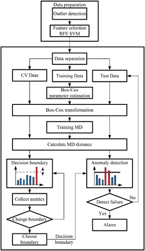
After HDD dataset is preprocessed, it is split into three subsets: training set, cross-validation set and test set. The training set contains only SMART parameter from healthy drives. Data values from training set are used to determine referent value for each SMART parameter based on the healthy data. Since SMART data are typically non-parametrically distributed, training set is also used to determine the appropriate power exponent λ for each of the parameters in order to transform data values of every attribute to be normally distributed. Transformed training data is further used for determining the center of mass of healthy data, in order to measure Mahalanobis distance of all data points in the two other subsets. Cross-validation set contains both data points from healthy and failed drives and is used to determine the most appropriate decision boundary which will achieve 0% FAR and the maximum value of FDR. Decision boundary is selected as value for predefined range which achieves minimum FAR on cross-validation set. Selected decision boundary is used on the independent test set to determine precision of failure detection of the proposed anomaly detection model.

Results and Discussion

Machine learning-based HDD failure prediction models require a collection of datasets of SMART parameters collected from the large population of HDDs operating under similar conditions. Such datasets are typically collected by manufacturers during quality testing or in large data centers. In order to test the proposed method, we used dataset provided by Center for Magnetic Recording Research (CMRR) which is commonly used by researchers in this field to evaluate their failure prediction models. This dataset contains a relatively small number of samples (68411 data samples collected from 369 drives), where each contains a set of 59 SMART parameters. Authors of CMRR dataset don’t provide details about drive vendor and operating conditions of failed drives. The monitored SMART parameters include temperature data, read and write error rates, head fly heights, servo and other parameters. HDD stores the last 300 SMART data samples in local memory collected in two-hour intervals, which are the last 600 hours of drive performance. Healthy drives contain information of the last 600 hours of operation as they passed reliability demonstration test which is performed by the manufacturer in controlled environmental conditions. Drives which failed in operation are returned to the manufacturer by users and some of them clocked less than 600 hours of operation. Dataset is collected from 191 failed drives which contain 17601 data samples and from 178 healthy drives which contain 51350 data samples.

SMART parameters included in dataset are as follows:

• FlyHeight – proportional to distance between HDD head and rotating plate.

• Servo – parameter related to head actuator

• CSS (Contact Start/Stop) – number of power supply interruptions, which forced heads to be parked in HDD landing zone.

• PList (Primary list) – list of defective sectors mapped during factory production tests

• GList (Grown list) – list of defective sectors mapped during operation by disk microcode

• Temp – various temperature readings of HDD components

• ReadErrors – number of incorrectly read sectors which had CRC (Cyclic Redundancy Check) error Writes/Reads – total number of write/read operations

Some of the SMART parameters in dataset which had constant values throughout the whole dataset were removed, such as Servo4, ReadError13, ReadError14, ReadError15 and ReadError16. Also, we observed that many parameters had a large number of zero-counts, with just few garbage values in failed part of the dataset, and they were removed. After this step, we were able to further remove eight parameters with constant values (Temp2, Temp5, Temp6, FlyHeight14, FlyHeight15, FlyHeight16, ReadError20, WriteError) thus further reducing computational complexity of the proposed model. Additionally, some of the abnormal values from remaining 46 parameters were removed using statistical outlier test. The dataset with these 46 features was fed to SVM-RFE feature selection algorithm proposed in (Wang, Miao, and Pecht 2011). This algorithm ranks features of a classification problem which is trained using SVM classifier with a linear kernel. Iteratively, the feature with smallest ranking criterion obtained by decision hyperplane was removed the algorithm being repeated until the most influential feature remained. Results presented in Table 1. represent 46 features which are ranked according to their importance when trained with linear SVM algorithm. The selected features presented are consistent with features selected by other researchers using various feature selection techniques.

Table 1. Features ranked by SVM RFE by their importance

Feature rank	Feature name	Feature rank	Feature name
1.	GList1	24.	FlyHeight5
2.	GList3	25.	CSS
3.	Servo10	26.	PList
4.	ReadError18	27.	Servo2
5.	Servo9	28.	Writes
6.	FlyHeight1	29.	ReadError3
7.	FlyHeight2	30.	ReadError2
8.	Temp4	31.	ReadError5
9.	FlyHeight11	32.	ReadError9
10.	Servo5	33.	FlyHeight7
11.	FlyHeight10	34.	FlyHeight4
12.	ReadError19	35.	Servo7
13.	Servo6	36.	Temp3
14.	FlyHeight9	37.	Servo3
15.	FlyHeight6	38.	ReadError1
16.	ReadError4	39.	ReadError7
17.	Servo1	40.	ReadError6
18.	FlyHeight12	41.	ReadError11
19.	FlyHeight8	42.	GList2
20.	Temp1	43.	ReadError12
21.	FlyHeight13	44.	Servo8
22.	Reads	45.	ReadError10
23.	FlyHeight3	46.	ReadError8

The dataset, containing 191 failed and 178 healthy drives, is divided into three randomly created subsets: training set, CV set and test set. These sets are formed in the following manner:

• Training set contains data from 106 randomly chosen healthy drives (roughly 60% data samples from healthy drives) and no data from any failed drives.

• Cross Validation (CV) set contains data from 36 randomly chosen healthy drives (roughly 20% data samples from healthy drives) and data from 95 randomly chosen failed drives (roughly 50% data samples from failed drives).

• Test set includes data from 36 randomly chosen healthy drives (roughly 20% data samples from healthy drives) and data from 96 randomly chosen failed drives (roughly 50% data samples from failed drives).

Many of the parameters in dataset are non-parametrically distributed (Schroeder and Gibson 2007), so we employed Box-Cox power transformation which finds the most appropriate power transformation coefficient lambda used to perform identical mathematical operation on each piece of original data, transforming data for normal distribution. The Box-Cox power transformation supports positive data greater than zero, thus data of each attribute is added to one prior the transformation so as to avoid problems with zero values parameters.

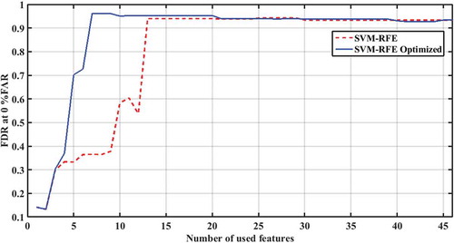
After the Box-Cox power transformation, dataset is normalized using mean and standard deviation of healthy drives from the training set in order to eliminate the effect of scaling. As the dataset contains some of the parameters with constant values for healthy drives, the marginal amount of Gaussian noise is added to them in order to avoid singularity problems when calculating covariance matrix. Mahalanobis distance (MD) is the distance between a certain point in multivariate space and the center of mass point. Based on the training set, Mahalanobis distance is calculated for all data from dataset and each data sample is represented by the single value which represents MD from the center of mass point. Anomaly detection algorithm is trained using MD values from cross-validation set. The goal of the algorithm is to choose decision threshold ε such that we have maximum score of some criterion. In practice, the most acceptable criterion is that each healthy drive is labeled correctly, which prevents false alarms (0% FAR). Decision boundary ε is determined using the two-step approach. The first element from the logarithmic scale within the range [10⁻³ ÷ 10¹²], which achieves 0% FAR, is chosen as course value for decision boundary. Next, new linear scale, bounded by coarse decision boundary value and its previous element, is divided into 1000 elements, where the first one achieving 0% FAR is chosen as the final value for decision boundary ε. The selected decision boundary ε value is used to evaluate the performance of the proposed failure detection algorithm on the test set. In order to determine the number of features needed to achieve the best performance of anomaly detection method, we iteratively added one additional feature from the SVM-RFE feature list then repeated the process of finding optimal decision boundary and finally tested the selected decision boundary on the test set. The broken red line in Figure 3 shows how FDR is affected by adding new features from the SVM-RFE feature list. As shown in the graph, maximum FDR result was achieved with 13 features, while further adding of the lower-ranked features to anomaly detection model gave almost constant results.

Figure 3. Failure detection rate in function of number of selected features

In order to eliminate the influence of dataset partitioning on the precision of failure prediction, results were obtained using ten experiments with randomly formed sets. With these 13 features, our anomaly detection algorithm, achieved averagely 94.32% FDR, with 0% FAR on seven tests, as shown in the left half of Table 2. In three other tests, our model reached 94.11% FDR, however was able to achieve 1.1% FAR.

Table 2. Test results for regular and optimized SVM RFE ranked features

Test No.	SVM RFE		Optimized SVM RFE
	FAR (%)	FDR (%)	FAR (%)	FDR (%)
1	0	95.79	0	94.74
2	0	95.79	0	98.94
3	0	92.63	0	96.84
4	0	90.53	0	94.74
5	1.14	91.58	0	96.84
6	0	95.97	0	95.79
7	0	93.68	0	94.74
8	1.09	95.97	0	95.79
9	1.09	94.79	0	97.89
10	0	95.79	0	94.79
Average	0	94.52	0	96.11

We observed that some features, highly ranked by SVM-RFE, made no contribution to the performance of anomaly detection method according to their expected rank. Those features were identified as: FlyHeight2, FlyHeight8, FlyHeight9, ReadError18, ReadError19 and Servo 9. When these features were added to the model, overall performance of anomaly detection algorithm stagnated or even decreased. In order to optimize anomaly detection method, these features were moved to the end of feature rank list as the ones with little relevance, as shown in Table 3.

Table 3. SVM-RFE feature rank list after optimization

Feature rank	Feature name	Feature rank	Feature name
1.	GList1	24.	ReadError2
2.	GList3	25.	ReadError5
3.	Servo10	26.	ReadError9
4.	FlyHeight1	27.	FlyHeight7
5.	Temp4	28.	FlyHeight4
6.	FlyHeight11	29.	Servo7
7.	Servo5	30.	Temp3
8.	FlyHeight10	31.	Servo3
9.	Servo6	32.	ReadError1
10.	FlyHeight6	33.	ReadError7
11.	ReadError4	34.	ReadError6
12.	Servo1	35.	ReadError11
13.	FlyHeight12	36.	GList2
14.	Temp1	37.	ReadError12
15.	FlyHeight13	38.	Servo8
16.	Reads	39.	ReadError10
17.	FlyHeight3	40.	ReadError8
18.	FlyHeight5	41.	FlyHeight2
19.	CSS	42.	ReadError19
20.	PList	43.	ReadError18
21.	Servo2	44.	Servo9
22.	Writes	45.	FlyHeight9
23.	ReadError3	46.	FlyHeight8

Subsequent to the optimization of feature list ranked by SVM-RFE we repeated the tests by iteratively adding one additional feature from the optimized SVM-RFE feature list, repeated the process of finding optimal decision boundary and tested the selected decision boundary on the test set. The results presented by solid blue line in Figure 3 show that maximum value of FDR is achieved by only seven features. The used features ranked by their importance were as follows: GList 1, GList 3, Servo 10, FlyHeight1, Temp4, FlyHeight11 and Servo5. The results show that the optimization of rank list reduced the number of the required features by half and still higher FDR was achieved. When seven features from the optimized rank list were used, our algorithm achieved 96.11% FDR with 0% FAR in all the ten tests, as presented in right half of Table 2.

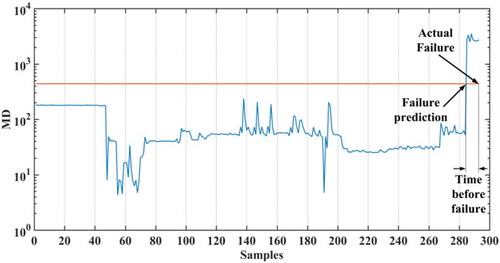
Besides the accurate prediction of HDD failure, it is important to highlight that the prediction is made in advance, before the failure actually occurs, which allows for timely data backup. As soon as the value of drives Mahalanobis distance exceeds threshold alarm is triggered predicting failure, as shown in Figure 4. The results presented in Table 4 show that our model was able to predict 80.53% failures at least 24 hours prior the occurrence of actual HDD failure. Our results are comparable to the results presented by GMFD (Queiroz et al. 2017) and these two methods both outperform TSP (Wang et al. 2014) and FSMD (Wang et al. 2013) failure prediction methods. Our algorithm was able to detect failure averagely 140 hours prior the occurrence of actual failure.

Table 4. Summary of time before failure for failed drives

Time before failure	Percentage
	OUR	GMFD	TSP	FSMD
Non-detectable	3.89	7.79	31.58	32.98
≥ 0	96.11	92.21	68.42	67.02
≥ 12 h	86.53	86.39	50.00	60.21
≥ 24 h	80.53	81.88	46.05	52.66
≥ 36 h	74.95	76.55	43.42	45.12
≥ 48 h	67.89	73.19	32.89	37.58

Figure 4. Failure prediction for drive #10

Conclusion

In this paper, we presented HDD failure prediction model which enables the user to take preventive actions in order to backup important data before failure actually occurs. Our model achieved averagely 96.11% failure detection rate, with 0% false alarms. The results of our tests showed better performance on identical CMRR dataset, in comparison with GMFD failure detections model which yielded 92.21% FDR (Queiroz et al. 2017), as well as TSP (Wang et al. 2014) and FSMD (Wang et al. 2013) models which achieved 68.42% FDR and 67.02% FDR, respectively. Furthermore, our model required only seven features, which is the half of features required by GMFD model and only a quarter of features required by TSP and FSMD models. With the reduced number of features, our model was easier to implement given the significantly reduced computational complexity, compared to other models.

Acknowledgments: This work was supported by the Ministry of Education and Science of the Republic of Serbia under Grants TR32043 and III43002 for the period 2011–2018.

References

- Agarwal, V., C. Bhattacharyya, T. Niranjan, and S. Susarla. 2009. Discovering rules from disk events for predicting hard drive failures, in Proceedings of the International Conference on Machine Learning and Applications, Miami Beach, Florida, USA, DOI: 10.1109/ICMLA.2009.62
- Appuswamy, R., R. Borovica, G. Graefe, and A. Ailamaki. 2017. The five minute rule thirty years later and its impact on the storage hierarchy, in Proceedings of the 7th International Workshop on Accelerating Analytics and Data Management Systems Using Modern Processor and Storage Architectures, Munich, Germany, 1–8
- Box, G., and D. Cox. 1964. An analysis of transformations. Journal of the Royal Statistical Society 26 (2):211–52. 1964.
- Cheng, S., and M. Pecht. 2012. Using cross-validation for model parameter selection of sequential probability ratio test, expert systems with applications. An International Journal Archive 39 (9):8467–73. doi:10.1016/j.eswa.2012.01.172.
- Chou, Y. M., A. Polansky, and R. Mason. 1998. Transforming non-normal data to normality in statistical process control. Journal of Quality Technology 30 (2):133–41. doi:10.1080/00224065.1998.11979832.
- Goldszmidt, M. 2012. Finding soon-to-fail disks in a haystack, in Proceedings of the 4th USENIX conference on Hot Topics in Storage and File Systems, Boston, MA, USA,
- Guyon, I., J. Weston, S. Barnhill, and V. Vapnik. 2002. Gene selection for cancer classification using support vector machines. Machine Learning 46(1/3):389–422. 1–3. doi:10.1023/A:1012487302797.
- Hamerly, G., and C. Elkan. 2001. Bayesian approaches to failure prediction for disk drives, in Proceedings of the Eighteenth International Conference on Machine Learning, San Francisco, CA, USA, 202–09,
- Hughes, G., J. Murray, K. Kreutz-Delgado, and C. Elkan. 2002. Improved disk-drive failure warnings. IEEE Transactions on Reliability 51 (3):350–57. doi:10.1109/TR.2002.802886.
- Kohavi, R. 1995. A Study of cross-validation and bootstrapping for accuracy estimation and model selection, in Proceedings of the 14th international joint conference on Artificial intelligence - 2, Montreal, Quebec, Canada,1137–43
- Mahdisoltani, F., I. Stefanovici, and B. Schroeder. 2017. Improving storage system reliability with proactive error prediction, 2017 USENIX Annual Technical Conference (USENIX ATC ’17). July 12–14, 2017,Santa Clara, CA, USA, ISBN 978-1-931971-38-6, pp. 391-402
- Murray, J., G. Hughes, and K. Kreutz-Delgado. 2003. Hard drive failure prediction using non-parametric statistical methods, in Proceedings of ICANN/ICONIP 2003, Istanbul, Turkey
- Murray, J., G. Hughes, and K. Kreutz-Delgado. 2005. Machine learning methods for predicting failures in hard drives: a multiple-instance application. The Journal of Machine Learning Research 6:783–816.
- Pitakrat, T. A., V. Hoorn, and L. Grunske. 2013. A comparison of machine learning algorithms for proactive hard disk drive failure detection in Proceedings of the 4th international ACM Sigsoft symposium on Architecting critical systems, Vancouver, British Columbia, Canada, 1–10, ISBN: 978-1-4503-2123-5, DOI: 10.1145/2465470.2465473
- Qian, J., S. Skelton, J. Moore, and H. Jiang. 2015. P3: Priority based proactive prediction for soon-to-fail disks, in Proceedings of the International Conference on Networking, Architecture and Storage (NAS), Boston, MA, USA, DOI: 10.1109/NAS.2015.7255224
- Queiroz, L., F. Rodrigues, J. P. P. Pordeus Gomes, F. T. Brito, I. Chaves, M. Paula, M. Salvador, and J. Machado. 2017. A fault detection method for hard disk drives based on mixture of gaussians and nonparametric statistics. IEEE Transactions on Industrial Informatics 13 (2):542–50. doi:10.1109/TII.2016.2619180.
- Schroeder, B., and G. Gibson. 2007. Disk failures in the real world: What does an MTTF of 1,000,000 hours mean to you?, in Proceedings of the 5th USENIX Conference on File and Storage Technologies (FAST 2007), San Jose, USA, 1–16
- Tan, Y., and X. Gu. 2010. On predictability of system anomalies in real world, in Proceedings of the International Symposium on Modeling, Analysis & Simulation of Computer and Telecommunication Systems (MASCOTS), Miami Beach, Florida, USA, DOI: 10.1109/MASCOTS.2010.22
- Wang, Y., E. Ma, T. Chow, and K. L. Tsui. 2014. A two-step parametric method for failure prediction in hard disk drives. IEEE Transactions on Industrial Informatics 10 (1):419–30. doi:10.1109/TII.2013.2264060.
- Wang, Y., Q. Miao, E. Ma, K. L. Tsui, and M. Pecht. 2013. Online anomaly detection for hard disk drives based on mahalanobis distance. IEEE Transactions on Reliability 62 (1):136–45. doi:10.1109/TR.2013.2241204.
- Wang, Y., Q. Miao, and M. Pecht. 2011. Health monitoring of hard disk drive based on Mahalanobis distance, in Proceedings of the Prognostics and System Health Management Conference, Shenzhen, China, DOI: 10.1109/PHM.2011.5939558
- Xu, Y., K. Sui, E. Yao, H. Zhang, Q. Lin, Y. Dang, P. Li, K. Jiang, W. Zhang, J. G. Lou, et al. 2018. Improving service availability of cloud systems by predicting disk error, Proceedings of the 2018 USENIX Conference on Usenix Annual Technical Conference, Boston, MA, USA. 481–493.
- Zhao, Y., X. Liu, S. Gan, and W. Zheng. 2010. Predicting disk failures with HMM- and HSMM-based approaches, in Proceedings of 10th Industrial Conference on Data Mining, ICDM 2010: Advances in Data Mining. Applications and Theoretical Aspects, Berlin, Germany, 390–404
- Zhu, B., G. Wang, X. Liu, D. Hu, S. Lin, and J. Ma. 2013. Proactive drive failure prediction for large scale storage systems, in Proceedings of the 29th Symposium on Mass Storage Systems and Technologies (MSST), Long Beach, CA, USA, DOI 10.1109/MSST.2013.6558427