Unmanned Aerial Vehicle Acoustic Localization Using Multilayer Perceptron

ABSTRACT

Unmanned Aerial Vehicles (UAVs), in recent years, are developing rapidly. However, when fly into private residences or public areas without authorizations, UAVs pose latent threats to personal privacy and public security. UAVs localization is a significant part of an anti-UAV system. In this paper, a remolded acoustic energy decay model preserved relative in acoustic energy attenuation inverse of distance square is used to generate training data. Multilayer perceptron(MLP) is the model to train these data and predicts accurate relative 3D space coordinates. Four different UAV flight trajectories are simulated. We also test robustness against noise with different levels. Simulation experiment results show that the deviation is less than 1.48 m in specific distances and noise levels, even with higher noise levels the deviation can still be accepted. The problem of limited detection range is overcome by the use of wireless sensor networks (WSNs) with more sensors. Long and short-term memory (LSTM) is investigated, but it doesn’t outperform MLP in accuracy and processing time.

Introduction

Unmanned Aerial Vehicle(UAV), a kind of small and remotely controlled aircraft, has been widely used in the agriculture, transportation and photography industry and is favored by the majority of aerial photographers. The number of users of UAV will continue to increase over upcoming years because the cost and the technical threshold of manufacturing UAV is reducing (Sedjelmaci, Senouci, and Ansari 2017).

Nonetheless, danger also comes with it. In 2018, a weaponized UAV attacked the Venezuelan president. This incident has aroused widespread public awareness about UAV’s latent danger. With the growing concerns regarding the safety issues of UAV, the anti-UAV system needs to be deployed significantly in protected space. An anti-UAV system has the ability to detect UAV once it flies into protected area and estimate its location for UAV defense (Shi et al. 2018).

UAV localization is a significant part of an anti-UAV system. There are many mature solutions for UAV detection. Such as video processing which uses convolutional neural network(CNN) to identify whether a UAV has break into the protected space (Rozantsev et al. 2016), but it cannot obtain the exact location of that UAV. Juhyun Kim et al. developed a UAV sound detection system which has performed FFT on sound data and then used Plotted Image Machine Learning and K Nearest Neighbors to analysis FFT graph (Kim et al. 2017), but this system can’t locate the UAV. The approach of choice for localization can be divided into three categories by measuring three types of physical variables: direction of arrival (DOA), time delay of arrival(TDOA) and signal strength or power of sensor received (Sheng and Hu 2007). The DOA techniques can be obtained by measuring the phase difference at different receiving sensors in the same time (Jensen et al. 2016). The TDOA can be estimated by time delay among different sensors (Lei, Cao, and Wei 2016). DOA-based methods are applicable for narrow-band signals. TDOA can be used for broadband source. Both DOA and TDOA requires high precision hardware in order to get the accuracy time point when the sensors receive the signal. The accuracy time is hard to define because the UAV as our target should be detected and recognized first. But, the length of time for processing detection and recognition is not constant, so the time point is blur. That will result in the predicted location getting large deviation for ground truth. Radar based on the micro-Doppler can achieve high detection and positioning accuracy, but it needs expensive devices to implement and might be not appropriate in crowded urban areas due to its high electromagnetic energy (Farlik et al. 2017).

Deep learning methods are being widely used in the solution of engineering problems. Multilayer perceptron(MLP) can learn the mapping from input to output through forward and back propagation. MLP is applied to the classification and prediction of various engineering problems, and has achieved remarkable performance. For example, Satar Mahdevari used MLP to predict the stability of gate roadways in longwall mining (Mahdevari et al. 2017), Abdi-Khanghah used MLP to predict solubility of N-alkanes in supercritical CO₂ (Abdi-Khanghah et al. 2018). Long and short-term memory (LSTM), which is able to connect previous position information to present task, is a popular algorithm. LSTM has better prediction on time series models, such as stock price prediction (Yu and Yan 2019). The prediction of the location of the drone flight is also a time series.

Hence, in this paper, we present a novel approach to estimate the UAV location using MLP based on acoustic energy measured at individual sensors in WSNs, which belongs to the third approach. The acoustic signals are produced by different components of UAV including propeller blades harmonics, hull vibration and engine noise (Jensen et al. 2016). The audio surveillance systems which use a network of tetrahedron acoustic arrays to receive signal suffer from a limited detection range (Azari et al. 2018; Christnacher et al. 2016). Due to that drawback, we introduce wireless sensor networks(WSNs) utilized as a strategy to expand the detection range. And LSTM is investigated in this task.

The main contributions of this paper are summarized as follows:

• Real-time UAV localization by MLP,

• Prediction relative 3-D space coordinates of UAV,

• Expansion the protected arrange using WSNs with more sensors.

This paper is organized as follows: Section 2 briefly formulates the acoustic energy decay model for location in WSNs. We train a simple multilayer perceptron to predict the location of UAV. In sSection 3, we introduce our simple multilayer perceptron and implementation details. Experiments and simulations are provided in sSection 4. Section 5 concludes the paper and points out possible feature work.

Acoustic Energy Decay Model

Sensor nodes, sink nodes and mange nodes constitute the WSNs. Sensor nodes are deployed in detected range in order to collect signal. When collecting signal, sensor nodes send the signal to neighbor nodes, then the neighbor nodes transmits up to sink nodes, which is designed to bring the information of nearby nodes together, until all information is transmitted to the mange node or base station. Mange nodes or base stations are responsible for processing these information for specific task. In this paper, we use WSNs to monitor protected areas.

The model below is widely used for acoustic signals (Chen et al. 2011; Sheng and Hu 2003). The acoustic signal received by sensors $y_i$, for i= 1, …, N., can be expressed as:

(1) $y_i=\frac{g_{i}P}{{∥x-s_i∥}^2}+{\epsilon }_i$(1)

Where $y_i$ represents the acoustic intensity which i-th sensor get, $g_i$is the gain factor of the i-th sensor, $P$ denotes the intensity of the source signal measured at a location with distance of 1 meter from the source, $x$ is the position of UAV, the square is the distance between the i-th sensor and source and ${\epsilon }_i$is modeled as a zero-mean additive white Gaussian (AWGN) noise with variance ς².

(2) $y_i=max\left(P\left(1-\alpha {∥x-s_i∥}^2\right)+n{\epsilon }_i,0\right)$(2)

We consider the effect of acoustical energy attenuation, in the same time, omitting the effect of the gain factor of sensors. A variation of the preceding Equation (1)(1) $y_i=\frac{g_{i}P}{{∥x-s_i∥}^2}+{\epsilon }_i$(1) can produce Equation (2)(2) $y_i=max\left(P\left(1-\alpha {∥x-s_i∥}^2\right)+n{\epsilon }_i,0\right)$(2) . Equation (2)(2) $y_i=max\left(P\left(1-\alpha {∥x-s_i∥}^2\right)+n{\epsilon }_i,0\right)$(2) can preserve relation in acoustic energy attenuation inverse of distance square and be more computationally attractive in WSNs due to limited resources for sensing, communication and computation. $\alpha$denotes the attenuation factor which depends on pressure and humidity of the measured environment. All the subtracted items represent the attenuated sound energy. This equation also preserves the AWGN. In practice, the signal strength each sensor obtained must be larger than zero, so we add a max function in order to compare the intensity of attenuated signal with zero. $n$ denotes the level of noise. In sSection 4, we will test robustness against noise with different levels.

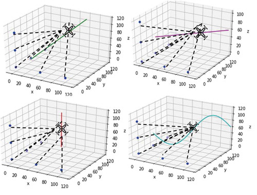
As shown in Figure 1, 7 WSNs nodes which are denoted by blue dots are distributed in limited spaces with single UAV flight path. We simulate UAV flight path with 3-D sin curve. 13 WSNs nodes are also simulated in sSection 4. Each node can receive acoustic signal that is produced by UAV. The acoustic signal mainly comes from propeller blades harmonics. The hull vibration and engine noise of UAV can also make noise. The node at the origin is as manage node. The distance between UAV and manage node is a relative distance which is used to estimate the detection range.

Figure 1. WSNs nodes position distribution and UAV flight path

Source Localization: Multilayer Perceptron

We presume that the intensity of flying quadrotor UAV acoustical power can be detected by sensors in protected space.

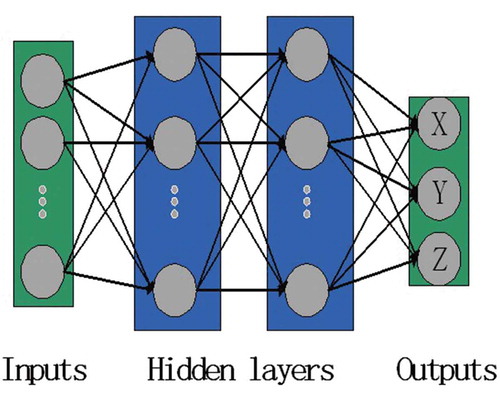
Our MLP network has four dense layers and the number of units in each layer is 256, 128, 64, and 3, as shown Figure 2. Each neuron in each layer has a similar formula expressed as:

(3) $a_j^{[l]}=\sigma (\sum _k{w}_{jk}^{[l]}{a}_k^{[l]}+b_j^{[l]})$(3)

Figure 2. Architecture of MLP network

Where $l$denotes $l$-th layer, $k$denotes the number of neurons in the upper layer, $j$denotes the number of neurons in the current layer. $w$and $b$represent weights and bais, respectively. $\sigma$ denotes activation function. $a$represents the activation value. Relu is the activation function and placed between output of front layer and input of next layer. We use Rectified Linear Units(ReLU) as activation function. ReLU can increase MLP module nonlinearity without increasing the computational complexity. In addition to the fourth layer, other layers have activation function. Because the fourth layer is the output layer used to output 3-D space coordinates, the number of its units has to be three. In mathematics, as the number of layer increases, the effect should be better, because the front layer is the subspace of the back layer. In simple words, when weights of back layer are constant one and biases are constant zero, the results should not be worse. But in practice, results are just opposite. More layers may make final predictive performance worse and bring about overfitting. For the reason that our acoustic energy decay model is not complex, we only use four layers to constitute MLP network. Many researchers have proved that more layers cannot achieve better performance which requires extend training time and leads to overfitting. Our simple network achieves outstanding performance instead.

We use deep learning framework Mxnet to construct MLP network. MLP network needs to be initialized before performing forward propagation. The Xavier is an effective random initialization method and is used in our network. Xavier initialization can increase convergence speed in initial iteration. The number of epochs is set to 8 K. We compare L1Loss that is the absolute value of the difference between the output and true label with L2Loss that is the square of them. The results of L1Loss and L2Loss are approximation. The approach of optimization is critical for convergence rate and result. Stochastic Gradient Descent (SGD) is a optimization algorithm which is widely utilized in Deep Learning (Neyshabur, Salakhutdinov, and Srebro 2015). The goal of SGD is to minimize the L2Loss value. SGD has a hyperparameter which is called learning rate. The learning rate requires a suitable value, otherwise the speed of convergence is slow or the optimization result cannot reach the global minimum. We use other fancy optimization algorithm named Adam (Kingma and Ba 2014). Adam can reduce the impact of learning rate on optimization performance. Adam has three hyperparameters. We keep two of the hyperparameters as defaults, just as the creator of Adam recommend. We only tune the remaining hyperparameter learning rate. The learning rate is set to 3e-4 from 0 to 6 K. From 6 K to 8 K, the learning rate reduces to 3e-5. We compare SGD with Adam. When we optimize MLP with SGD, the loss has been falling, but the rate of decline is very small. Even 8 K epochs have run out, loss value was larger than one with 4 K epochs using Adam optimizer. Therefore, we utilize Adam as optimizer method in this model.

We use the data generated by remolded acoustic energy decay model as raw input data. And we simulate the position of the UAV with several different flight trajectories and use three-dimensional coordinates of that position as raw label data. Before transferred into MLP network, the raw input data need to be preprocessed first. Data preprocessing plays a key supporting role in the implementation of this algorithm. Without data preprocessing, the loss function is hard to converge. With regard to raw label data, an approach used frequently is to process the logistic regression labels by logarithm. These treatments correspond to:

(4) $x_i=\frac{{\hat{x}}_i-\mu }{\sigma }$(4)

(5) $y_i=log({\hat{y}}_i)$(5)

Where $\mu$and$\sigma$represent mean and standard deviation, respectively. ${\hat{x}}_i$ denotes the raw inputs date and $x_i$ denotes input data, the rest can be deduced by analogy. The processed data have an adverse effect on subsequent predictions, that will be discussed in sSection 4. After weighing the merits and drawback, we still choose preprocessing raw data before training the model.

LSTM is a variant of the Recurrent Neural Network (RNN) and explicitly designed to avoid the long-term dependency problem. LSTM consists of forget gate, input gate and output gate. The first step is the forget gate which decides what information we are going to throw away. The second step is the input layer that decides what new information we are going to store. The last step is the output layer which decides what parts of the information we are going to output. The units of LSTM in each layer is same as MLP. The output layer is also Dense layer with three units. All the optimizer, initialization, learning rate and loss function are same as MLP network.

Experiments and Results

In this section we will introduce dataset and hardware we used in our experiments. We used 4 different trajectories to simulate UAV flight path. Three common UAV flight modes automatic takeoff and landing, automatic returning and oblique fly are simulated by vertical line, horizontal line and slash line respectively. In addition, we also simulate complex flight path with 3-D sin curve. In mathematics, sin curves of different frequencies and amplitudes can be linearly combined into arbitrary curves. Therefore, if our model can achieve high accuracy in 3-D sin curve, validation of our method can be proved. Concerning the training of MLP, we use nn.Block of Mxnet to build network. The configurations of the computer used in this research, they are: CPU: Intel(R) Xeon(R) E5-2640 v4, 2.40 GHz and GPU: Nvidia Tesla P100, 12GB. GPU is not very important in this study and almost impossible to speed up training. Using only CPU is fine.

We use acoustic energy measured from the individual sensor nodes in the coverage field to locate the targets in region as raw input. The 3-D space coordinates will be produced after input through MLP as sSection 3. Batch normalization doesn’t help due to shallow frame, neither does weight decay and dropout. The processing time for each epoch is 0.46s.

We assume that the protected area is a space with a length, width and height of 100 m. UAV flies vertically upwards for a distance, when it takes off. And when UAV lands, it flies vertically downwards with slower speed. We can simulate automatic takeoff and landing with a vertical line that fixes the x, y-axis coordinates. In same MLP network, the loss value can be reduced to 2.48e-4.

When the UAV flies farther, the user wants it to automatically return to the starting point safely. He can choose automatic returning, then the UAV will fly horizontally in one direction at a fixed altitude. We utilize horizontal line that is parallel to soy plane and fixed z-axis coordinates. In same MLP network, the loss value can be reduced to 2.75e-4.

Another common flight path is oblique flight that can make x, y, z axes change simultaneously. We use slash line which is x, y, and z axes changing at different rates at the same time. In same MLP network, the loss value can be reduced to 1.87e-4.

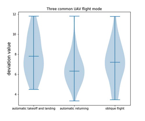
As shown in Figure 3, we use violin-plot to show the distribution of three common UAV flight path deviation value. The simulation of automatic takeoff and landing has maximum deviation and its average value is close to 8.0. Most of its values are distributed between 6.0 and 8.0. The simulation of automatically return has maximum deviation and its average value is slightly larger than 6.0. Only a small percentage of values are larger than 8.0, most of values are distributed near its average. The violin-plot of oblique flight is slender, and its average is approximately equal to 7.0. The means of three common UAV flight deviation value correspond to their loss value. Though the difference among their loss value are smaller than 0.0001, the prediction of them may be larger than 1.0. This large contrast is the numerical stability problem caused by the logarithm of the label as described in sSection 3. The cause of this problem is the derivative of the exponential function is large, and the output of MLP network should do exponential transformation to get real 3-D coordinate.

Figure 3. Deviation value of three common UAV flight mode

We focus on the analysis of sin curves. We divide the distance between the UAV and the manage node into three stages. The first stage is the distance between 10 m and 65 m. The second stage is the distance between 65 m and 120 m, and the third stage is the distance between 120 m and 170 m. The following Table 1 gives a summary of all deviation range of three stages. The first row denotes distance between manage node and UAV which is also three stages. The first column denotes number of nodes plus levels of noise. We use different $n$ in Equation (2)(2) $y_i=max\left(P\left(1-\alpha {∥x-s_i∥}^2\right)+n{\epsilon }_i,0\right)$(2) to set levels of noise as described in section 2. The value in table is accurate because we exclude mutation values. As we can see, the smallest value is 1.48 which means that the deviation can limit to 1.0 in the second stage. When the noise level rises to 2.5, the accuracy rate is basically not falling. When the noise level rises to 5.0, the deviation of the third stage is twice as much as the former one. The strange phenomenon is that the minimum deviation arranges shift from the second stage to first stage. When the noise level rises to 10.0, the deviation can be restricted below 3.90. But when the noise level rises to 25.0, The test results are extremely unstable. Sometimes the deviation is below 1.0, but it may rise dramatically to 100.0. Nan stands for values greater than 25.0. The fastest flight speed of DJI UAV can achieve 20 m/s (products @ www.dji.com n.d.), so when the prediction of our MLP network is 25.0 larger than true label. When the distance exceeds 170 m, the deviation is quite large, and the prediction loses its meaning.

Table 1. Deviation range of prediction coordinate using MLP with 7 nodes

	10 ~ 65	65 ~ 120	120 ~ 170
7 + 1.0	1.74	1.48	4.42
7 + 2.5	1.68	2.20	4.74
7 + 5.0	3.52	4.60	11.86
7 + 10.0	7.22	3.90	12.32
7 + 25.0	Nan	18.8	Nan

The second stage is generally lower than the first and third stage. At the first stage, the distance is insufficient to distinguishing the sound intensity difference. However, the results in the third stage is susceptible to noise interference due to a long distance. The problem of it should be cured, if we distribute more nodes to receive sound signal.

For this purpose, we increase the number of nodes to 13 and keep the original node position unchanged. Theoretically speaking, the results should not be worse than network with 7 nodes. As shown in Table 2. Even in case of 1.0 noise level, the deviation is generally larger. When the noise level rises to 5.0, the deviation rapidly expands. In contrary to this trend of increasing deviation, when the noise level rises to 10.0, accuracy rate suddenly becomes normal. The first stage becomes a more accurate prediction range. As respect to MLP network with 13 nodes, low-level noise has a big impact on the results. The noise of each node accumulates into huge deviation. However, when the noise takes a large proportion, MLP network could strip noise from a constant sound source of UAV through multiple layers of forward propagation. If the number of feature isn’t enough, perhaps MLP network can not recognize main signals. And if the level of noise is low, MLP network may take all signals as UAV signal without noise interference.

Table 2. Deviation range of prediction coordinate using MLP with 13 nodes

	10 ~ 65	65 ~ 120	120 ~ 170
13 + 1.0	3.78	9.62	14.12
13 + 2.5	9.34	22.9	23.28
13 + 5.0	Nan	Nan	Nan
13 + 10.0	2.96	3.12	9.42
13 + 25.0	8.94	16.61	18.84

LSTM is investigated in the same sin 3-D data. The loss values with noise levels of 1.0, 2.5, 5.0, and 10.0 reduce to 0.0058, 0.0342, 0.0860, and 0.2320, respectively. And the processing time for each epoch is 1.95s. The prediction of 1.0 noise level is larger than 25 m, others are more terrible. In theory, LSTM can connect the information in long or short time steps. The position of the last time step of the UAV should be related to the next moment. So LSTM should do better than MLP. But, the experiment result shows that LSTM does not perform as well as shallow MLP network in our task.

Conclusion and Future Work

In this paper, we propose a method localize UAV real-time by MLP based on acoustic energy. We remolded the acoustic energy decay model that preserves relative in acoustic energy attenuation inverse of distance square and which is also more computationally attractive in WSNs. We use this decay model to generate four different kinds of curves data that denote four different UAV flight trajectories, and use them as training date. The curves are 3-D sin, vertical line, horizontal line and slash line and the latter three represent automatic takeoff and landing, automatic returning and oblique fly respectively. MLP network can predict accurate relative 3D space coordinates after training. Our experiments cover the comparisons of positioning accuracy under different levels of noise. Based on the results obtained, our method has high localization accuracy and better noise-suppression characteristics. This study serves as a guidance for UAV localization that plan to defeat intruder UAV. However, the assumption is made on the number of objects to be tracked limited to a UAV. Our method cannot detect the presence of UAV and is not applicable when multiple UAVs appear. In the feature, an end-to-end detection and localization of UAV based on recurrent neural network (Jeon et al. 2017), which is able to analyze the sound signal to identify UAV, will be explored.

References

- Abdi-Khanghah, M., A. Bemani, Z. Naserzadeh, and Z. Zhang. 2018. Prediction of solubility of N-alkanes in supercritical CO2using RBF-ANN and MLP-ANN. Journal of CO2 Utilization 25 (November2017):108–19. doi:10.1016/j.jcou.2018.03.008.
- Azari, M. M., H. Sallouha, A. Chiumento, S. Rajendran, E. Vinogradov, and S. Pollin. 2018. Key technologies and system trade-offs for detection and localization of amateur drones. IEEE Communications Magazine 56 (1):51–57. doi:10.1109/MCOM.2017.1700442.
- Chen, J., C. Wang, Y. Sun, and X. Shen. 2011. Semi-supervised Laplacian regularized least squares algorithm for localization in wireless sensor networks. Computer Networks 55 (10):2481–91. doi:10.1016/j.comnet.2011.04.010.
- Christnacher, F., S. Hengy, M. Laurenzis, A. Matwyschuk, P. Naz, S. Schertzer, and G. Schmitt. 2016. Optical and acoustical UAV detection (Invited Paper). Electro-Optical Remote Sensing X.
- Farlik, J., M. Kratky, J. Casar, and V. Stary. 2017. Radar cross section and detection of small unmanned aerial vehicles. International Conference on Mechatronics-Mechatronika, Prague, Czech Republic.
- Jensen, J. R., J. K. Nielsen, R. Heusdens, and M. G. Christensen. 2016. DOA estimation of audio sources in reverberant environments. IEEE International Conference on Acoustics, Shanghai, China.
- Jeon, S., J.-W. Shin, Y.-J. Lee, W.-H. Kim, Y. H. Kwon, and H.-Y. Yang. 2017. Empirical study of drone sound detection in real-life environment with deep neural networks.
- Kim, J., C. Park, J. Ahn, Y. Ko, J. Park, and J. C. Gallagher. 2017. Real-time UAV sound detection and analysis system. SAS 2017-2017 IEEE Sensors Applications Symposium, Proceedings, 1–5. doi:10.1109/SAS.2017.7894058.
- Kingma, D. P., and J. Ba. 2014. Adam: A method for stochastic optimization. 1–15. http://arxiv.org/abs/1412.6980.
- Lei, Y., J. Cao, and Y. Wei. 2016. TDOA location based on modified Newton method. IEEE International Conference on Signal Processing.
- Mahdevari, S., K. Shahriar, M. Sharifzadeh, and D. D. Tannant. 2017. Stability prediction of gate roadways in longwall mining using artificial neural networks. Neural Computing and Applications 28 (11):3537–55. doi:10.1007/s00521-016-2263-2.
- Neyshabur, B., R. Salakhutdinov, and N. Srebro. 2015. Path-SGD: Path-normalized optimization in deep neural networks. International Conference on Neural Information Processing Systems, Montreal, Canada.
- products @ www.dji.com. n.d.. https://www.dji.com/cn/products#drones-nav.
- Rozantsev, A., S. N. Sinha, D. Dey, and P. Fua. 2016. Flight dynamics-based recovery of a UAV trajectory using ground cameras. doi:10.1109/TPAMI.2016.2564408.
- Sedjelmaci, H., S. M. Senouci, and N. Ansari. 2017. Intrusion detection and ejection framework against lethal attacks in UAV-aided networks: A Bayesian game-theoretic methodology. IEEE Transactions on Intelligent Transportation Systems 18:1143–53. doi:10.1109/TITS.2016.2600370.
- Sheng, X., and Y. H. Hu. 2003. Energy based acoustic source localization. International Conference on Information Processing in Sensor Networks, Berlin, Germany.
- Sheng, X., and Y.-H. Hu. 2007. Energy based acoustic source localization. 285–300. doi:10.1007/3-540-36978-3_19.
- Shi, X., C. Yang, W. Xie, C. Liang, Z. Shi, and J. Chen. 2018. Anti-drone system with multiple surveillance technologies: Architecture, implementation, and challenges. IEEE Communications Magazine 56 (4):68–74. doi:10.1109/MCOM.2018.1700430.
- Yu, P., and X. Yan. 2019. Stock price prediction based on deep neural networks. Neural Computing and Applications. doi:10.1007/s00521-019-04212-x.