A New Spatio-Temporal Neural Network Approach for Traffic Accident Forecasting

ABSTRACT

Traffic accidents forecasting represents a major priority for traffic governmental organisms around the world to ensure a decrease in life, property, and economic losses. The increasing amounts of traffic accident data have been used to train machine learning predictors, although this is a challenging task due to the relative rareness of accidents, inter-dependencies of traffic accidents both in time and space, and high dependency on human behavior. Recently, deep learning techniques have shown significant prediction improvements over traditional models, but some difficulties and open questions remain around their applicability, accuracy, and ability to provide practical information. This paper proposes a new spatio-temporal deep learning framework based on a latent model for simultaneously predicting the number of traffic accidents in each neighborhood in Madrid, Spain, over varying training and prediction time horizons.

Introduction

Nowadays, the urbanization trend around the globe has introduced new opportunities and issues in the cities. One of the most important aspects of modern society is related to the use of motorized vehicles as a method of transport. Although very efficient in several ways (Litman 2009), motor vehicles imply problems related to traffic and health care. For example, pollution and traffic accidents are some of the principal causes of death in cities all over the world (Kelly and Fussell 2015; WHO 2015).

This is the reason why the scientific interest for traffic accidents has increased in the past decades, and proposing solutions is a crucial issue for the sake of improving transportation and public safety. Being capable of understanding and reducing accidents has become an important commitment in many cities, as they not only cause significant life losses, but also property and economic ones (Peden et al. 2004).

In this work, an effort will be put to study the traffic accident phenomenon in the city of Madrid, Spain. This has been the subject of several lines of research in the past, although most previous studies on traffic accident prediction conducted by domain researchers simply applied classical prediction models on limited data without addressing many challenges properly, thus leading to unsatisfactory performances. For instance, the imbalanced severity classes, nonlinear relationship between dependent and independent variables, or spatial heterogeneity are usual problems to deal with in order to improve previous results in the field. Even with an accurate and complete statement of the problem, human and external factors (roads, vehicles, etc.) make this field highly challenging (Hoel et al. 2011; Vaa, Penttinen, and Spyropoulou 2007).

Although predicting the exact space-temporal position of accidents is out of the scope with actual techniques due to its complexity (Mannering and Bhat 2014; Zhang, Yau, and Chen 2013), much progress might be done by characterizing important parts of the problem. Trying to reduce the dimensionality of the space as much as possible, discovering relevant features or improving previous models are some examples of what can be done to provide insight in this particular problem.

In this context, this work presents the problem as a spatio-temporal series in which traffic intensity and meteorological variables play a central rol in predicting values for the traffic accidents series. For this purpose, we propose a new model, called XSTNN (from Exogenous Spatio-Temporal Neural Network) that consists of a deep learning approach for traffic accident regression based on spatio-temporal data. The model, which extends the Spatio-Temporal Neural Network (STNN) proposed by Delasalles et al. (2019) through the addition of external variables, is based on partitioning space into grid cells and taking advantage of the spatial relations existing in the series. A number of urban and environmental variables such as traffic intensity, rainfall, temperature, and wind are collected and map-matched with each grid cell. Given the number of accidents as well as the other urban and environmental features at each location, we learn a model to forecast the number of accidents that will occur in each grid cell in future timesteps.

By presenting the number of traffic accidents as a spatio-temporal series and learning how to model it, it is possible (for example) to increase emergency service’s response time, focus the efforts to avoid potential dangers, create real-time safe routes recommendation systems, and, in short, reduce the losses that were discussed above. To the best of our knowledge, this is the first work that tackles the traffic accident forecast problem in the city of Madrid, although the proposed framework can be easily extend to any particular zone.

The rest of the paper is organized as follows: related work is discussed in Section 2, while Section 3 presents our datasets and the problem formulation. Section 4 introduces our deep learning model for traffic accident regression and Section 5 illustrates the evaluation of the proposed architecture as derived after appropriate experimentation. Finally, in Section 6 we point out future research directions and conclusions.

Related Work

Although very much studied, traffic accidents have been treated mostly in a “classical” context, by simply using statistical analysis in an attempt to understand better the phenomenon and the circumstances surrounding them. Examples that illustrate this situation can be found in Abdel-Aty and Radwan (2000), Lord (2006), and Roshandeh, Agbelie, and Lee (2016). There also are several works dealing with these methodologies and their typical issues (as for example Lord and Mannering 2010; Mannering and Bhat 2014). A long list of studies tackle the issue from the severity of the injuries perspective. Within this last group, de Oña, Mujalli, and Calvo (2011, 2013), Galatioto et al. (2018), Meysam et al. (2015), and Qiu et al. (2014) are some examples. Although instructive, most of these previous research fail to be able to apply all this knowledge to predict future events.

In a closer line to our work, during the last decade a considerably number of Artificial Intelligence-based approaches have appeared, taking advantage of the large datasets which are available nowadays. We can cite Chen (2017), Li et al. (2008), Lin, Wang, and Sadek (2015), and Zhang et al. (2018) as examples. As a first glance in the matter, these works provide new tools for solving the problem, but they lack relevant information in their analysis and mainly focus in showing the better performance of an specific model, without deepening in the behavior of their algorithms. However, there are some counterexamples like Tarek and Walid (1998), where a fair comparison is made between neural and fuzzy models in the field of traffic accident. In order to get more sophisticated and precise systems, last researches focus their efforts in new models as Variational Autoencoders, Deep Neural Networks, and video-based models for detecting and understanding better traffic accidents (Singh and Mohan 2019; Yu, Xu, and Gu 2019; Zheng et al. 2019).

Until now, the references presented here did not tackle the regression problem or were all lumped under the same hypothesis: ignoring the importance of the spatial dimension in the traffic accidents forecasting. However, a number of studies have pointed out how relevant this variable is in order to get appropiate results (Xu and Huang 2015; Rhee et al. 2016). Since then, more and more researches focus their efforts in the spatio-temporal (and not just temporal) prediction problem. We can cite Ren et al. (2017), Yang, Wang, and Yu (2018), and Yuan, Zhou, and Yang (2018) as some of the most relevant works, some of them being classified under the label of Deep Learning. Specifically, some of these last references point at exogenous variables as helpful in the forecast process.

While traffic accident research from an Artificial Intelligence perspective per se is still a young field, its importance makes them be a central variable of a vast number of Intelligent Transport Systems studies. For example, several of them in which routes recommendation systems and vehicle routing problems are stated, identify traffic accidents as potential variables that might have direct impact in the system. Is the case of Eshtehadi, Demir, and Huang (2020), the routing problem is tackled by an adapted adaptive large neighborhood search algorithm. Similarly, Du et al. (2019) focus their efforts in solving a similar problem but trying to minimize the total transportation risk, time and cost by using an improved biogeography-based optimization algorithm. As the authors point out, when transporting hazardous materials traffic accidents might suppose a great risk. In Salman and Alaswad (2018), a model based on Markov chain for traffic optimization to decrease congestion is presented. In those cases, although unpredicted traffic pattern changes are contemplated, a robust traffic accident forecasting system could be beneficial. In the same way, Sumit and Akhter (2019) show that traffic accidents might be a main actor for road weight calculation. By using a c-means clustering and deep-neurofuzzy model, they use (among other variables) real-time accident data for detecting traffic congestion, monitoring traffic status, and deciding optimum route. Another example can be found in Nasri, Bekta¸s, and Laporte (2018), where it is showed another field that could benefit from traffic accident research: autonomous vehicles and their anticipation to potentially dangerous situations. Cunneen et al. (2019) show how Artificial Intelligence could also contribute in the ethical aspects of this matter. In this same context, Liu et al. (2016) propose V2I communications between vehicles in order to improve traffic condition. Particularly, an accident prediction system could refine future vehicle’s decisions.

Problem Formulation and Data

Problem Formulation

Given a spatial grid $S$, where each grid is represented as $s_i$, and a timestep $t_j$, we aim to learn a model to predict the number of accidents in each grid $s_i$ during each time slot $t_j$. This mean that a spatio-temporal sample writes as $x(s_i;t_j):j=1,\dots ,T;i=1,\dots ,S$.

Although spatial zones might be defined arbitrarily, it is expected that using intrinsic spatial information could be helpful. More precisely, we propose that each grid $s_i$ represents a neighborhood of Madrid as it is expected that each neighborhood presents different peculiarities that might be related to traffic accidents. Moreover, we use an hour as the length of our timestep $t_j$. Without loss of generality, other values could be chosen for $s_i$ and $t_j$. We work with data from year 2018 for both the training and validation sets. Only in-city accidents are treated, as road accidents present different peculiarities.

For the rest of the section, all the data cleaning and manipulation will take into consideration this proposed framework.

Data Sources

• Traffic accident data: Provided by Portal de datos abiertos del Ayuntamiento de Madrid,¹ it summarizes all the information related to car crashes in the city of Madrid. Specifically, for every accident it shows physical location (although not geographycal), date (year, month, and day), time (hour), sex and severity for each person involved and several meteorological conditions. The last two variables of this dataset were not taken in consideration, as they were not relevant or there were better sources for them (concretley weather data later in this same section). For example, sex can be relevant when making statistics of the phenomena, but irrelevant when trying to predict new accidents.

Spatial information is presented as city addresses (street and number or intersection), while temporal information is limited to the hour in which the accident was reported.

• Traffic data: As before, provided by Portal de datos abiertos del Ayuntamiento de Madrid. This dataset contains historical data of traffic measurement points in the city of Madrid. The measurements are taken every hour at each point, including traffic intensity in number of cars per hour and average speed in m/s. Some other traffic parameters, although unused in this project, are present in this set too.

Spatial information is given with the coordinates (longitude and latitude) of measurement points, while temporal information is taken every 15 minutes.

• Weather data: Weather data were provided by the Red Meteorológica Municipal.² Weather observations consist of hourly temperature in Celsius degrees, solar radiation in W/m2, wind speed measured in ms-1, wind direction in degrees, daily rainfall in mmh-1, pressure in mbar, degree of humidity in percentage, and ultraviolet radiation in mWm-2 records.

Weather information is taken along six different stations. It is reported hourly.

Some cleaning work was necessary to work through the data. It is worth noting that these decisions are fundamental as error might be introduced in the system during this cleaning process.

Firstly, Google Maps Api³ was used for geocoding the adresses provided in the dataset.

With respect to traffic intensity, it is worth pointing out that is the only set that does not present its information hourly, but every 15 minutes. In order to have a final homogeneus dataset, average over every entire hour is calculated. Note that typical deviation of traffic intensity over and hour represents less than $10\mathrm{\%}$ of the real values on average. In addition, the average of the traffic intensity is taken for each neighborhood as if every measurement point was a different sample from the same phenomenon for every zone. Once more, the standard deviation that results from this decision is less than $5\mathrm{\%}$ respect to the mean, showing that there is a predisposition to have similar traffic conditions for each neighborhood.

Finally, while the actual meteorological data were taken in six substations in the city of Madrid, our own data consist of average hourly variables from those six substations. Although this decision could be seen as a loss of information, this approximation is enough for a first insight. Also, assigning different meteorological variables for each accident depending on its location supposes an extra difficulty when using a spatial mesh (the six substations) different from the one used in this work (neighborhoods of Madrid).

Data Analysis

Through this section, we will explore if our data can be modeled as a spatio-temporal series. This will be done by an exploratory analysis for both dimensions.

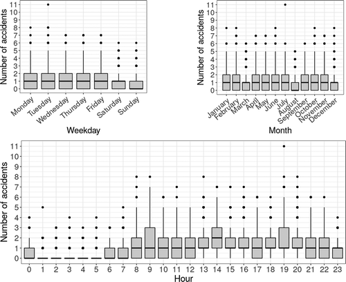
To explore its time dependency, it is possible to use a boxplot of different time windows of traffic accident count for different time periods of Madrid as in Figure 1. Clearly, the traffic accident patterns change drastically for different time periods. Specifically, traffic accidents are more frequent at traffic rush hours than that at off-peaks, on weekdays than on weekends, and they reflect a decrease in summer holiday days. This figure reveals some characteristical periodicities that expose a hidden time dependence in traffic accidents, letting us model the series as a temporal one.

Figure 1. Periodicities of the traffic accidents series. (a) Number of accidents depending on day of the week. Weekends present less number of accidents. (b) Number of accidents for each month. August seems to be safer. (c) Number of accidents depending on hour of the day. In this case we have the most clear difference

To determine whether the number of traffic accidents is associated with the spatial location, the heatmap of number of traffic accidents is plotted for Madrid in 2018 (Figure 2). As it can be seen, the number of traffic accidents is not uniformly distributed, and it is highly related with the geographical position of a neighborhood. Usually, the neighborhoods with highest traffic accident concentrations lie in the major commercial and business areas.

Figure 2. Total number of accidents by neighborhoods of Madrid during 2018

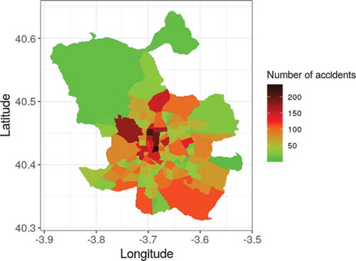
From this two last figures, we can point out one of the special difficulties of the traffic accidents series: how infrequent accidents are. In this context, and from the frequentist probability point of view, the odds of an accident taking place anytime in an hour and at any neighborhood is about $0.8\mathrm{\%}$.

Deep Model for Traffic Accident Forecasting

This paper presents a new deep learning neural model which is based on the work from Ziat et al. (Delasalles et al. 2019). Specifically, they introduced a method for spatio-temporal series forecasting problems, such as meteorology, oceanography, or traffic, formalized as a recurrent neural network for modeling time-series of spatial processes. Our model preserves this nature but it is an improvement from the point of view of its usability, allowing us to make use of external (or exogenous) variables. Concretely, the model learns these spatio-temporal dependencies through a structured latent dynamical representation, while a decoder predicts the observations from the latent space.

Notation

Let us first introduce the notation that will be used througout this chapter. Denoting $n$ as the number of series, $T$ their length and $m$ the dimensionality of them. In our specific domain, there will be as many series ($n$) as spatial zones. Moreover, $m=1$ as every series will be composed of only one dimension: traffic accidents.

If we call $X$ as the values of all the series between instants 1 and $T$, then $X$ is a tensor in ${\mathbb{R}}^{T\times n\times m}$. At last, $X_t\in {\mathbb{R}}^{n\times m}$ is a tensor that denotes the values of all the series at time $t$.

The STNN Model

Let $Z_t$ be the latent representation, or latent factors, of the series at time $t$. The model has two principal components: the dynamic function (denoted as $g$), and the decoder function (called $d$). The first one is in charge of controlling the dynamics of the system, calculating the next latent state based on the previous one: $Z_{t+1}=g(Z_t)$. The second one is a decoder which maps latent factors $Z_t$ onto a prediction of the actual series values at time $t$: ${\tilde{X}}_t=d(Z_t)$, ${\tilde{X}}_t$ being the prediction computed at time $t$.

As it should be clear, the parameters of both functions ($g$ and $d$) are learned so that the essence of the series is captured. Unlike usual neural networks, the latent representation $Z_t$ is treated as a parameter too, distinguishing this model and making it more flexible than usual recurrent neural networks.

The idea behind the spatial component is to consider each zone as a different series with its own latent representation at each time step. For a latent space dimension of $N$, $Z_t$ is a $n\times N$ tensor such that $Z_{t,i}\in {\mathbb{R}}^N$ is the latent factor of series $i$ at time $t$. Thus, we have the following relations:

(1a) $d:{\mathbb{R}}^{n\times N}\to {\mathbb{R}}^{n\times m}$(1a)

(1b) $g:{\mathbb{R}}^{n\times N}\to {\mathbb{R}}^{n\times N}$(1b)

Not only each spatial zone has a series, spatial information is integrated in the dynamic component of the model through a matrix $W\in {\mathbb{R}}_{+}^{n\times n}$ that shares information between all the zones. Although this matrix will be provided, the actual model is also capable of learning it.

The latent representation of each series at time $t+1$ depends on the previous state of all the series (included itself). Hence, we can separate the calculation of a new state by two different sources: intra-dependency in the first term of the right-hand side of (3) and inter-dependency in the second term. The first one aims to get the dynamic of each series as an individual entity, whereas the second one is devised to exploit spatial relations between all series. This way, the model considers a different temporal series in each spatial zone while keeping information about the spatial relation between all of them. Formally, the dynamic model $g(Z_t)$ is designed as follows:

(2) $Z_{t+1}=h(Z_t{\mathrm{\Theta }}^{(0)}+W{Z}_t{\mathrm{\Theta }}^{(1)})$(2)

In this last equation, $h$ is a nonlinear function ($h=tanh$ in this project) and $\mathrm{\Theta }$ denotes a parametrized function $\mathrm{\Theta }\in {\mathbb{R}}^{N\times N}$. In this case, $\mathrm{\Theta }$ will be a linear function or a multilayer perceptron (MLPs), although could be any parametrized function.

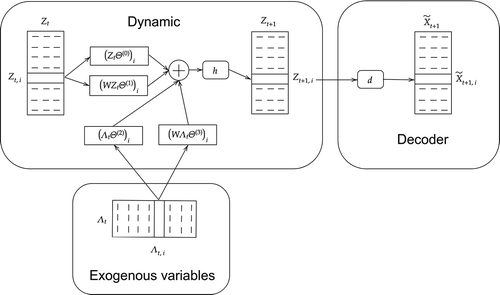
Including Exogenous Variables: The XSTNN Model

The main limitation of the STNN is that it is not able to take into account the exogenous variables which might be related to the process being modeled and which could enrich the internal representation and, thus, improve the predictions. The XSTNN aims to resolve this.

Let us denote the exogenous variables $\mathrm{\Lambda }$. The main idea will be to change equation 2(2) $Z_{t+1}=h(Z_t{\mathrm{\Theta }}^{(0)}+W{Z}_t{\mathrm{\Theta }}^{(1)})$(2) so that the latent space is modified directly by $\mathrm{\Lambda }$. These variables are temporal series, so they can be treated on the same way we did previously, meaning that ${\mathrm{\Lambda }}_t$ denotes the slice of $\mathrm{\Lambda }$ at time $t$. Due to the possibility of using several exogenous variables, ${\mathrm{\Lambda }}_t$ is a $n\times m$ tensor.

By introducing $\mathrm{\Lambda }$ in the estimation of $Z_t$, the model learns the dynamics taking into account external information too. As the premise of this work is to assume that exogenous variables might change the dynamic of the series, learning to mold the system in function of both meets our requirements the best.

Once the main idea has been explained, it is necessary to answer some other questions. Concretely, there are a few alternatives for reconstructing (2) in the way it was intended. Moreover, a discussion about what time step to use with $\mathrm{\Lambda }$ is desirable: when computing $Z_t$, both ${\mathrm{\Lambda }}_t$ and ${\mathrm{\Lambda }}_{t+1}$ might be beneficial. The first one represents the idea of a previous state having an effect on the next one, whereas the second option symbolizes the conception of an actual state modifying the series.

Let us now introduce some possibilities. First, if exogenous data does not present spatial dependency, it can be more efficient to avoid the use of spatial relations for $\mathrm{\Lambda }$. This version writes:

(3) $Z_{t+1}=h(Z_t{\mathrm{\Theta }}^{(0)}+W{Z}_t{\mathrm{\Theta }}^{(1)}+{\mathrm{\Lambda }}_t{\mathrm{\Theta }}^{(2)})$(3)

On the contrary, when exogenous variables may exhibit spatial dependency, the same treatment that $Z$ has will be provided to $\mathrm{\Lambda }$. This notion is captured as follows:

(4) $Z_{t+1}=h(Z_t{\mathrm{\Theta }}^{(0)}+W{Z}_t{\mathrm{\Theta }}^{(1)}+{\mathrm{\Lambda }}_t{\mathrm{\Theta }}^{(2)}+W{\mathrm{\Lambda }}_t{\mathrm{\Theta }}^{(3)})$(4)

A diagram that represents this last option is presented in Figure 3.

Figure 3. Architecture of the XSTNN model as described in Sect. 4.3

Overall, the model is similar to the STNN. Both the optimization problem and the training (loss function, learning algorithm, inference, etc.) are applicable to the XSTNN model.

However, we would like to point out the two principal limitations of our proposal:

• Using an specific matrix $W$ for a concrete problem means that, for different circumstances (for example, a different spatial grid), a retraining is needed.

• Both the dynamic and the decoder functions are stationary, meaning that it do not change over time. In Delasalles et al. (2019) a method to tackle this problem is proposed.

Experimental Results

Before explaining the experiments, we will establish what questions we wish to answer. They are stated as follow: (1) Are the results of the proposed model better when compared with benchmark methods, including classical predictive models, tree-based models and STNN? (2) Is our proposed model capable of managing different spatial regions or timesteps? (3) Do the forecasting results make sense? Does our model provide more insights on the problem? (4) Are the predicted accident locations correlated with the ground truth spatially?

Through these questions, we expect to evaluate if the XSTNN model supposes a step forward in the prediction of traffic accidents.

Baselines Models and Evaluation Metrics

Several methods have been chosen to be compared with the XSTNN. Concretely, the STNN itself, a XGBoost tree-based algorithm (Chen and Guestrin, 2016), linear regression, and a naive mean and persistence models. The mean model forecasts new values of the series using the mean of past values from the same series, while persistence model uses the last value for each series for making the prediction.

To evaluate the accuracy and precision of the prediction, we selected Mean Absolute Error (MAE) and Bias as our metrics. In a spatio-temporal context (Wikle, Zammit-Mangion, and Cressie 2019), they are defined as:

(6) $\mathrm{M}\mathrm{A}\mathrm{E}=\frac{1}{TS}\sum _{j=1}^T\sum _{i=1}^S|x_{s_i;t_j}-{\tilde{x}}_{s_i;t_j}|$(6)

(7) $\mathrm{B}\mathrm{i}\mathrm{a}\mathrm{s}=\frac{1}{TS}\sum _{j=1}^T\sum _{i=1}^S(x_{s_i;t_j}-{\tilde{x}}_{s_i;t_j})$(7)

where, as it was defined in Section 2, $x(s_i;t_j):j=1,\dots ,T;i=1,\dots ,S$ is a spatio-temporal sample from the real series, $\tilde{x}(s_i;t_j)$ makes reference to the predicted series, $S$ is the total number of spatial grids and $T$ the total number of timesteps.

Performance Evaluation

To validate the different proposed methodologies, a time series cross-validation scheme called rolling origin is used (Tashman 2000). Rolling origin is an evaluation technique according to which the forecasting origin is updated successively and the forecasts are produced from each origin. This technique allows obtaining several forecast errors for time series, which gives a better understanding of how the models perform.

Let us now describe how the previous procedure is applied in our own experiments. Consider the following steps:

1. The traffic accidents dataset is splitted in ten succesive sets, that is to say, starting all sets from January, 1st of 2018 at 00:00, each of those ten sets end at a different date between February, 14th at 23:00 and December, 31st at 18:00. To consider, all datasets are equally spaced and a minimun of 45 days have been set for training.

2. As a test set, we consider predictions within a 5 hour horizon. For a train set of $T$ timesteps, this means that the evaluation of the quality of the model will be made over $T+1$ to $T+5$ timesteps.

3. Finally, the ten splitted sets are trained and validated over $T+1$ to $T+5$ timesteps. The final error is the average of all validations. The datasets have been chosen with the purpose that different hours and week days are tested for a more complete and extensible validation.

This procedure is equivalent for all models. It was applied to both the parameter tuning and the final training process.

Experimental Setup and Parameter Tuning

We set up the neural networks experiments and the other two models on a external machine proportionated by Departamento de Inteligencia Artificial, UNED .⁴ The STNN and the XSTNN⁵ were built upon PyTorch. Concretely, an early-stopping approach using Adam optimizer with the settings: ${\beta }_1=0.0$, ${\beta }_2=0.999$, $\in ={10}^{-9}$ and $w_d={10}^{-6}$ was used for both methodologies. The mean, persistence, linear regression, and XGboost models are built on R, the last one made use of the package xgboost (Chen and Guestrin, 2016).

With respect to parameter and hyper-parameter tuning, we grid-searched hyper-parameters on each models for the sake of achieving the best possible results. The final hyper-parameters used for this work are gathered in Table 1.

Table 1. Values used for each hyper-parameter. $n_z$ is the dimension of the latent space. The remaining variables were presented in Section 3 or are commonly used parameters

STNN	Learning rate	0.01
$\lambda$	0.01
$n_z$	2
$g(Z)$	Linear
Minibatch size	512
Dropout	0.25
XSTNN	Learning rate	0.01
$\lambda$	0.1
$n_z$	2
$g(Z)$	Linear
Minibatch size	512
Dropout	0.35
XGBoost	Number of rounds	80
Max. depth	15
$\eta$	0.1
$\gamma$	1
Min. child weight	1
Subsample	0.7

Any other hyper-parameter not taken into account in this tuning process, are used with their default values. We decided to set matrix $W$ (spatial relations, introduced in Section 3), as the inverse of spatial distance. Thus, all zones are in some way related but in a bigger degree the closer they are. Lastly, each series was rescaled between 0 and 1.

Results and Discussion

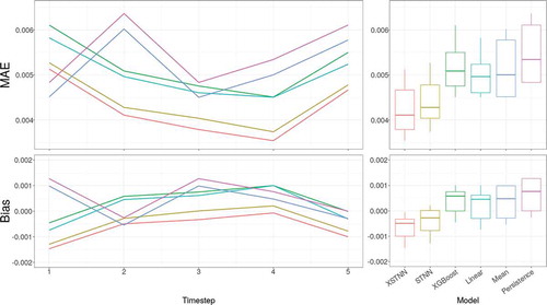
In order to identify quantitatively the performance of the different models and baselines, Table 2 provides the average prediction error for $T+1$ to $T+5$. From this first insight it should be clear that both XSTNN and STNN outperform the other models. As Mean model and XGboost were trained taking into account the existence of a spatial grid but without establishing relations between them, these results confirm that making use of prior spatial information is beneficial for the regression problem. Beyond that, the XSTNN presents a better performance than the STNN.

Table 2. Performance for $T+1$ to $T+5$ traffic accident regression

Model	MAE	Bias
XSTNN	$\mathbf{0}\mathbf{.0041}\pm \mathbf{0}\mathbf{.0006}$	$-0.0006\pm 0.0004$
STNN	$0.0045\pm 0.0006$	$-0.0004\pm 0.0006$
XGBoost	$0.0052\pm 0.0006$	$0.0004\pm 0.0006$
Linear regression	$0.0050\pm 0.0006$	$0.0002\pm 0.0007$
Mean	$0.0052\pm 0.0007$	$0.0003\pm 0.0007$
Persistence	$0.0055\pm 0.0008$	$0.0006\pm 0.0007$

For a more detailed vision, Figure 4 shows the distribution of the metrics and the average error by timestep. From this figure, same conclusions can be extracted as before: the XSTNN model presents a better general behavior compared to the rest of the models. Again, the fact of introducing spatial knowledge to the problem stands as an appropriated approach for this particular series, and our results reinforce the idea that introducing exogenous variables is favorable for the regression problem. However, it is worth noting that there is not a clear relation between errors and timestep. Although an increment on the error by timestep in the prediction is usually expected (cumulative error), the randomness of traffic accidents does not let us extract clear conclusions from this aspect.

Figure 4. Forecasting performance (MAE and bias) of the different models by timestep together with the calculated distributions

Beyond the quantitative analysis, now we show some accomplishments from our proposed model respect to the STNN. For that purpose, we will take a deeper look into a concrete example, without loss of generality.

Let us introduce the following situation: we forecast the accident regression series from $17$ p.m. to $21$ p.m. on a Wednesday. From Figure 1 we know this situation corresponds to a high-risk circumstance for traffic accidents to happen. In this context, Figure 5 illustrates a comparison of our two principal models with a levelplot (time in $x$ axis, neighborhoods in $y$ axis and colored by traffic accidents). Let us expose several ideas.

Figure 5. A practical example of the operation of both networks, XSTNN and STNN, for the same situation. From $17$ p.m. to $21$ p.m. on a Wednesday

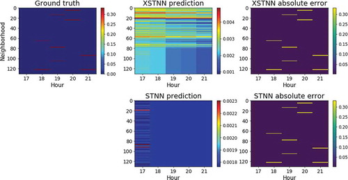
First of all, and unfortunately, the regression problem is far from being solved. A comparison of colorbars from both, STNN and XSTNN predictions, with the ground truth corroborates this statement. As Chen et. al. have documented, after some analysis of traffic accident data, it is difficult to predict whether traffic accidents will happen or not directly, because complex factors can affect traffic accidents, and some factors, such as the distraction of drivers, cannot be observed and collected in advance (Chen et al. 2016). Nevertheless, our XSTNN model has proved to be a new step in the right direction, outperforming the rest of baselines models (Table 2).

Secondly, the next natural question that rises is about the reason of this improvement. Again, Figure 5 sheds light on this matter. Whereas the STNN quiclky truncates its values close to $0$ for every neighborhood and timestep, the XSTNN takes some risks and it is able to differentiate between time intervals and spatial zones. As the most likely situation is having no accidents for each hour and neighborhood, both networks have values approaching to $0$ as outputs.

Certainly, taking more risks does not ensure a better performance in the regression problem. It is necessary that the model manages to elucidate which time intervals and neighborhoods are more important for the problem that we have in hand as a function of past events. In this concrete case, the model has learned to prioritize neighborhoods from 1 to 80, as they report a vast majority of the total number of traffic accidents in the city of Madrid. Besides, the XSTNN reveals a negative trend over the hours as we would expect.

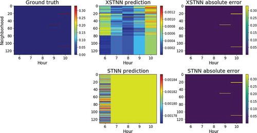
As XSTNN learns better to distinguish between time ranges and spatial zones, it is possible to find other situations in which, again, this model offers more information and assimilates the system’s dynamics in a better way. For example, and to corroborate that the XSTNN behaves better in a variety of situations, Figure 6 gives evidence of a totally different state on a Sunday from $6$ a.m. to $10$ a.m. In this context, we will expect a higher risk at last late hours and at past $9$ a.m., the XSTNN correspondingly adapting its output to this situation. On the contrary, the STNN is not capable of learning the corresponding dynamic. Unlike previously (Figure 5), this time the XSTNN takes less risks and its output is closer to 0 as we would expect less accidents on a Sunday morning that a Wednesday on the evening as before.

Figure 6. A practical example of the operation of both networks, XSTNN and STNN, for a same situation. From $6$ a.m. to $10$ a.m. on a Sunday

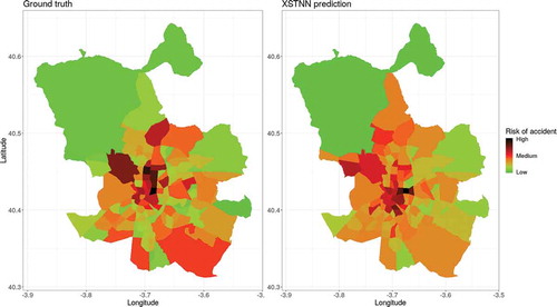
Through the previous discussion we have pointed out how the XSTNN infers properties based on the time condition and the concrete spacial zone. For this last case, Figure 7 offers an analysis of spatial risk for each neighborhood. Both series, the real and the predicted ones, were rescaled for a direct comparison between them. This way, it is clear that the XSTNN is capable of reasoning in both dimensions, temporal and spatial.

Figure 7. Spatial risk in the same scale for the ground truth (left) and the XSTNN (right)

In summary, the XSTNN reports a better understanding and learning of the dynamic of the system, being more flexible and creative in its prediction. These features translate into a better performance than their direct rivals.

Conclusions

Through this work, a new approach for spatio-temporal series forecasting called XSTNN has been proposed. The problem of traffic accidents prediction was tackled by this new neural network model, showing a better performance than the rest of baselines model. Also, the exposed model is easily extendable to any temporal or spatial configuration. Although traffic accidents regression is challenging due to several difficulties, the XSTNN has proved to stand out for its capability to provide a deeper insight in the problem series and to adapt its reasoning to a larger number of different situations. Thus, this paper demonstrates that spatio-temporal neural networks are a promising field for traffic accident prediction in the future.

Future work in this field can be extended to incorporate other features that are not necessarily series, like economics or demographics. Also, the XSTNN model might be extended by introducing more temporal terms from exogenous series for updating the latent space.

Additional information

Funding

This research was partially funded by the Empresa Municipal de Transportes (EMT) of Madrid under the program “Aula Universitaria EMT/UNED de Calidad del Aire y Movilidad Sostenible”.

Notes

1. https://datos.madrid.es/portal/site/egob/

2. http://www.mambiente.madrid.es

3. https://cloud.google.com/maps-platform/

4. http://www.ia.uned.es/

5. Code available at https://github.com/rdemedrano/xstnn

References

- Abdel-Aty, M. A., and A. E. Radwan. 2000. Modeling traffic accident occurrence and involvement. Accident Analysis & Prevention 32 (5):633–42. doi:10.1016/S0001-4575(99)00094-9.
- Chen, C. 2017. Analysis and forecast of traffic accident big data. In ITM Web of Conferences 12, 04029, Guangzhou (China).
- Chen, Q., X. Song, H. Yamada, and R. Shibasaki. 2016. Learning deep representation from big and heterogeneous data for traffic accident inference. In AAAI: Proceedings of the Thirtieth AAAI Conference on Artificial Intelligence. Phoenix, USA.
- Chen, T., and C. Guestrin. 2016. XGBoost: A scalable tree boosting system. In Proceedings of the 22nd ACM SIGKDD International Conference on Knowledge Discovery and Data Mining - KDD ‘16, 785–94, San Francisco, USA.
- Cunneen, M., M. Mullins, F. Murphy, and S. Gaines. 2019. Artificial driving intelligence and moral agency: Examining the decision ontology of unavoidable road traffic accidents through the prism of the trolley dilemma. Applied Artificial Intelligence 33(3):267–93. Publisher: Taylor & Francis eprint. doi:10.1080/08839514.2018.1560124.
- de Oña, J., G. López, and J. Abellán. 2013. Extracting decision rules from police accident reports through decision trees. Accident Analysis & Prevention 50:1151–60. doi:10.1016/j.aap.2012.09.006.
- de Oña, J., R. O. Mujalli, and F. J. Calvo. 2011. Analysis of traffic accident injury severity on spanish rural highways using bayesian networks. Accident Analysis & Prevention 43 (1):402–11. doi:10.1016/j.aap.2010.09.010.
- Delasalles, E., A. Ziat, L. Denoyer, and P. Gallinari. 2019 December. Spatio-temporal neural networks for space-time data modeling and relation discovery. Knowledge and Information Systems 61(3):1241–67. doi:10.1007/s10115-018-1291-x.
- Du, J., X. Li, L. Li, and C. Shang. 2019. Urban hazmat transportation with multifactor. Soft Computing 24, 6307–6328.
- Eshtehadi, R., E. Demir, and Y. Huang. 2020 March. Solving the vehicle routing problem with multi-compartment vehicles for city logistics. Computers & Operations Research 115:104859. doi:10.1016/j.cor.2019.104859.
- Galatioto, F., M. Catalano, N. Shaikh, E. McCormick, and R. Johnston. 2018 November. Advanced accident prediction models and impacts assessment. IET Intelligent Transport Systems 12(9):1131–41. doi:10.1049/iet-its.2018.5218.
- Hoel, J., M. Jaffard, C. Boujon, and P. Van Elslande. 2011. Different forms of attentional disturbances involved in driving accidents. IET Intelligent Transport Systems 5 (2):120. doi:10.1049/iet-its.2010.0109.
- Kelly, F. J., and J. C. Fussell. 2015. Air pollution and public health: Emerging hazards and improved understanding of risk. Environmental Geochemistry and Health 37 (4):631–49. doi:10.1007/s10653-015-9720-1.
- Li, X., D. Lord, Y. Zhang, and Y. Xie. 2008. Predicting motor vehicle crashes using support vector machine models. Accident Analysis & Prevention 40 (4):1611–18. doi:10.1016/j.aap.2008.04.010.
- Lin, L., Q. Wang, and A. W. Sadek. 2015. A novel variable selection method based on frequent pattern tree for real-time traffic accident risk prediction. Transportation Research Part C: Emerging Technologies 55:444–59. doi:10.1016/j.trc.2015.03.015.
- Litman, T. A. 2009. Transportation cost and benefit analysis: Techniques, estimates and implications, Victoria Transport Policy Institute, 2nd ed. 1-19.
- Liu, Y., J. Ling, Q. Wu, and B. Qin. 2016. Scalable privacy-enhanced traffic monitoring in vehicular ad hoc networks. Soft Computing 20 (8):3335–46. doi:10.1007/s00500-015-1737-y.
- Lord, D. 2006. Modeling motor vehicle crashes using poisson-gamma models: Examining the effects of low sample mean values and small sample size on the estimation of the fixed dispersion parameter. Accident Analysis & Prevention 38 (4):751–66. doi:10.1016/j.aap.2006.02.001.
- Lord, D., and F. Mannering. 2010. The statistical analysis of crash-frequency data: A review and assessment of methodological alternatives. Transportation Research Part A: Policy and Practice 44 (5):291–305.
- Mannering, F. L., and C. R. Bhat. 2014. Analytic methods in accident research: Methodological frontier and future directions. Analytic Methods in Accident Research 1:1–22.
- Meysam, E., R. M. Ali, H. Farshad, and S. Shahin. 2015 November. Prediction of crash severity on two-lane, two-way roads based on fuzzy classification and regression tree using geospatial analysis. Journal of Computing in Civil Engineering 29(6):04014099. doi:10.1061/(ASCE)CP.1943-5487.0000432.
- Nasri, M. I., T. Bekta¸s, and G. Laporte. 2018. Route and speed optimization for autonomous trucks. Computers & Operations Research 100:89–101. doi:10.1016/j.cor.2018.07.015.
- Peden, M., R. Scurfi, D. Sleet, D. Mohan, A. A. Hyden, and E. Jarawan. 2004. World report on road traffic injury prevention.
- Qiu, C., C. Wang, B. Fang, and X. Zuo. 2014. A multiobjective particle swarm optimization-based partial classification for accident severity analysis. Applied Artificial Intelligence 28(6):555–76. Publisher: Taylor & Francis eprint. https://www.tandfonline.com/doi/pdf/10.1080/08839514.2014.923166
- Ren, H., Y. Song, J. Wang, Y. Hu, and J. Lei. 2017. A deep learning approach to the citywide traffic accident risk prediction. In 2018 IEEE International Conference on Intelligent Transportation Systems (ITSC), Maui, Hawaii, USA.
- Rhee, K.-A., J.-K. Kim, Y.-I. Lee, and G. F. Ulfarsson. 2016. Spatial regression analysis of traffic crashes in seoul. Accident Analysis & Prevention 91:190–99. doi:10.1016/j.aap.2016.02.023.
- Roshandeh, A. M., B. R. D. K. Agbelie, and Y. Lee. 2016. Statistical modeling of total crash frequency at highway intersections. Journal of Traffic and Transportation Engineering (English Edition) 3 (2):166–71. doi:10.1016/j.jtte.2016.03.003.
- Salman, S., and S. Alaswad. 2018. Alleviating road network congestion: Traffic pattern optimization using Markov chain traffic assignment. Computers & Operations Research 99:191–205. doi:10.1016/j.cor.2018.06.015.
- Singh, D., and C. K. Mohan. 2019. Deep spatio-temporal representation for detection of road accidents using stacked autoencoder. IEEE Transactions on Intelligent Transportation Systems 20 (3):879–87. doi:10.1109/TITS.2018.2835308.
- Sumit, S. H., and S. Akhter. 2019. C-means clustering and deep-neuro-fuzzy classification for road weight measurement in traffic management system. Soft Computing 23 (12):4329–40. doi:10.1007/s00500-018-3086-0.
- Tarek, S., and A. Walid. 1998 January. Comparison of fuzzy and neural classifiers for road accidents analysis. Journal of Computing in Civil Engineering 12(1):42–47. doi:10.1061/(ASCE)0887-3801(1998)12:1(42).
- Tashman, L. J. 2000. Out-of-sample tests of forecasting accuracy: An analysis and review. International Journal of Forecasting 16 (4):437–50. doi:10.1016/S0169-2070(00)00065-0.
- Vaa, T., M. Penttinen, and I. Spyropoulou. 2007 June. Intelligent transport systems and effects on road traffic accidents: State of the art. IET Intelligent Transport Systems 1(2):81–88. doi:10.1049/iet-its:20060081.
- WHO. 2015. WHO | data.
- Wikle, C. K., A. Zammit-Mangion, and N. Cressie. 2019. Spatio-temporal statistics with R. 1st ed. Chapman and Hall/CRC, London, United Kingdom.
- Xu, P., and H. Huang. 2015. Modeling crash spatial heterogeneity: Random parameter versus geographically weighting. Accident Analysis & Prevention 75:16–25. doi:10.1016/j.aap.2014.10.020.
- Yang, K., X. Wang, and R. Yu. 2018. A bayesian dynamic updating approach for urban expressway real-time crash risk evaluation. Transportation Research Part C: Emerging Technologies 96:192–207. doi:10.1016/j.trc.2018.09.020.
- Yu, Y., M. Xu, and J. Gu. 2019. Vision-based traffic accident detection using sparse spatio-temporal features and weighted extreme learning machine. IET Intelligent Transport Systems 13 (9):1417–28. doi:10.1049/iet-its.2018.5409.
- Yuan, Z., X. Zhou, and T. Yang. 2018. Hetero-ConvLSTM: A deep learning approach to traffic accident prediction on heterogeneous spatio-temporal data. In Proceedings of the 24th ACM SIGKDD International Conference on Knowledge Discovery & Data Mining - KDD ‘18, 984–92. ACM Press, London, United Kingdom.
- Zhang, G., K. K. W. Yau, and G. Chen. 2013. Risk factors associated with traffic violations and accident severity in china. Accident Analysis & Prevention 59:18–25. doi:10.1016/j.aap.2013.05.004.
- Zhang, Z., Q. He, J. Gao, and M. Ni. 2018. A deep learning approach for detecting traffic accidents from social media data. Transportation Research Part C: Emerging Technologies 86:580–96. doi:10.1016/j.trc.2017.11.027.
- Zheng, M., T. Li, R. Zhu, J. Chen, Z. Ma, M. Tang, Z. Cui, and Z. Wang. 2019. Traffic accident’s severity prediction: A deep-learning approach-based CNN network. IEEE Access 7:39897–910. doi:10.1109/ACCESS.2019.2903319.