Near Real-time Map Building with Multi-class Image Set Labeling and Classification of Road Conditions Using Convolutional Neural Networks

ABSTRACT

Road Weather Information Systems (RWIS) provide real-time weather information at point locations and are often used to produce road weather forecasts and provide input for pavement forecast models. Compared to the prevalant street cameras, however, RWIS are sometimes limited in availability. Thus, extraction of road conditions data by computer vision can provide a complementary observational data source if it can be done quickly and on large scales. In this paper, we leverage state-of-the-art convolutional neural networks (CNN) in labeling images taken by street and highway cameras located across North America. The final training set included 47,000 images labeled with five classes: dry, wet, snow/ice, poor, and offline. The experiments tested different configurations of six CNNs. The EfficientNet-B4 framework was found to be most suitable to this problem, achieving validation accuracy of 90.6%, although EfficientNet-B0 achieved an accuracy of 90.3% with half the execution time. The classified images were then used to construct a map showing real-time road conditions at various camera locations. The proposed approach is presented in three parts: i) application pipeline, ii) description of the deep learning frameworks, iii) the dataset labeling process and the classification metrics.

Introduction

Adverse road conditions present a frequent hazard to motorists. In cold climates, snow, ice, and frost can produce slippery roads, while the reduced friction from wet roads is a hazard in both warm and cold climates. Data from 2010–2018 in the United States showed that on average 767,779 crashes per year (13% of the total) occur during adverse weather conditions (rain, snow, sleet, freezing rain, or hail). In addition, an average of 2,747 fatalities per year (9% of all fatalities) occurred during times of adverse weather conditions.¹ Advances have been made in better monitoring roads during hazardous weather conditions. Road Weather Information Systems (RWIS) can provide real-time road weather information at point locations, which is often used to produce road weather forecasts (e.g. (Crevier and Delage 2001; Sass 1997)). This data is then transmitted to transportation operations centers and disseminated to the public through services such as the 511 network (Drobot et al. 2014). Many RWIS are also equipped with cameras, which give a real-time view of the road. While the information provided by RWIS and cameras is useful, there are still limitations. Since these systems are operated at the state/province or local level, there is no unified road information system. Therefore, motorists must consult different sources for road weather information in each jurisdiction where they travel. Due to the cost of such systems, not all jurisdictions have RWIS/cameras and those that do often have a limited number. This can introduce large gaps in road weather information. These gaps are sometimes filled by manual observations from operators or have no data at all. Since cameras are much more prevalent than RWIS, and less expensive, they may present an opportunity to improve road weather data where there is currently limited data. In addition, since camera images are readily available and come in common formats, they can be sourced across all jurisdictions and combined into a unified system. However, combining all such cameras is a major task, since there are tens of thousands in North America alone. Furthermore, as noted by Carrillo et al. (Carrillo et al. 2019) it is challenging for operators to process vast amounts of road weather data in real-time.

As such, using the road conditions data extracted from these images on a large scale would not be possible for continuous monitoring applications, since the significant time delay caused by manual human extraction would mean the data is no longer “real-time.” In addition, the extraction of road conditions data, when done on a large scale, can provide a source of new observational data which can be assimilated into pavement forecast models, which normally use RWIS data as an input. Such pavement models require observed data, in close to real-time, to calibrate initial conditions (Crevier and Delage 2001). Therefore, it is of value from both a monitoring and forecasting perspective to quickly extract road conditions data on a large scale.

Early work involving road condition classification from weather data involved cameras mounted on vehicles and was primarily used in vehicle navigation (Almazan, Qian, and Elder 2016; Bronte, Bergasa, and Alcantarilla 2009; Gallen et al. 2011; Hautiere et al. 2006; Kurihata et al. 2005; Omer and Fu 2010; Pavlić et al. 2012; Roser and Moosmann 2008; Yan, Luo, and Zheng 2009; Zhang and Ma 2015). Some of these methods used image processing techniques such as extracting regions of interest (ROI) from the images or road segmentation. Histogram features derived from the ROIs can then be used with classical machine learning methods such as Support Vector Machines (SVM) to label the weather/road conditions into various categories such as sunny, cloudy and rainy. Road condition estimation based on this spatio-temporal approach to model wet road surface conditions, that integrates over many frames, was explored in (Amthor, Hartmann, and Denzler 2015). Weather recognition from general outdoor images was explored in (Laffont et al. 2014; Li, Kong, and Xia 2014; Narasimhan and Nayar 2003; Shen 2009; Song, Chen, and Gao 2014) to name a few.

The success of deep convolutional neural networks (DCNN) (LeCun, Bengio, and Hinton 2015; Schmidhuber 2015) in computer vision tasks (Krizhevsky, Sutskever, and Hinton 2012; Russakovsky et al. 2015), and the generation of large weather datasets (Lin et al. 2017; Lu et al. 2017; Zhao et al. 2018), led to their application in weather recognition problems (Elhoseiny, Huang, and Elgammal 2015; Li et al. 2018; Lin et al. 2017; Villarreal Guerra et al. 2018; Zhao et al. 2018; Zhu et al. 2016).

Automatic fog detection with DCNNs using the H20 platform² to predict the presence of dense fog from daytime camera images has been implemented with several sets of images collected by Royal Netherlands Meteorological Institute (KNMI) (Pagani, Noteboom, and Wauben 2018). To provide details, H20 is an open-source, distributed machine learning platform that supports most widely used and up-to-date machine learning and statistical algorithms incorporated with cutting edge AutoML³ technique that automatically searches for the best hyper-parameter combinations and produces a leaderboard of outperforming models. The combinations were explored at random, based on hyper-parameters space grid search accommodated by H20 library to select fog detecting model architectures that have the best F1 score for each data set. A near-real-time geographical map showing the predicted values of the cameras was also given with promising results.

In (Pan et al. 2018), 5000 images from highway sections in Ontario, Canada captured by smartphones were used to classify road surface conditions using a pre-trained VGG-16 model. For a five-class road surface classification, the best accuracy with DCNN was 78.5%. In (Nolte, Kister, and Maurer 2018), two DCNNS were applied to differentiate six classes of road surface conditions such as cobblestone, wet asphalt, snow, grass, dirt and asphalt with an eventual goal of predicting the road friction coefficient. This study augmented their dataset with data from publicly available datasets for automated driving, which led to a classification accuracy of 92%. Classification of road surface condition with deep learning models was explored by Carillo et al. (Carrillo et al. 2019) where six state-of-the-art DCNN models were pre-trained using ImageNet parameters to classify to road surface condition images (about 16,800) from roadside cameras in Ontario, Canada.

The research goals explored in this paper are as follows: i) to leverage state-of-the-art DCNN’s in labeling images taken by street and highway cameras located across Canada and the United States (see Figure 1), ii) to evaluate multiple DCNN models for classification of road conditions, and iii) to construct a real-time map of North-America depicting road conditions. The work reported in this paper was published in an open-access archive⁴ (Ramanna et al. 2020).

Figure 1. Sample raw images from street and road cameras representing (a) Dry (b) Offline, (c) Poor, (d) Snow and (e) Wet categories

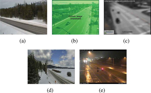
The training data for these experiments used images labeled as dry, wet, snow/ice, poor, and offline. The experiments tested different configurations of six convolutional neural networks (VGG-16, ResNet50, Xception, InceptionResNetV2, EfficientNet-B0 and EfficientNet-B4) to assess their suitability to this problem. The precision, accuracy, and recall were measured for each framework configuration. In addition, the training sets were varied both in overall size and by the size of individual classes. The final training set included 47,000 images labeled using the five aforementioned classes. The EfficientNet-B4 framework was found to be most suitable to this problem. It was observed that VGG-16 with transfer learning proved to be very useful for data acquisition and pseudo-labeling with limited hardware resources, throughout this project. The EfficientNet-B4 framework was then placed into a real-time production environment, where images could be classified in real-time on an ongoing basis.

The major contributions of this work are as follows: i) a methodology outlining steps for generating a multi-class dataset of images of road conditions in North America from road cameras, ii) detailed analysis of the process of semi-automated dataset labeling using well-known deep learning frameworks, and iii) deploying a production-level classifier for generating a map to display real-time road conditions. It is also noteworthy that the best classification accuracy result of 90.9% was achieved without performing any pre-processing on the images (such as noise removal, text/logo removal, histogram equalization, cropping) other than rescaling.

Our paper is organized as follows: In Section 2, we give an overview of the map building application pipeline and discuss the various convolutional network architectures used in this paper. In Section 3, we present a detailed discussion of the process of labeling raw images and generating training examples. In Section 4, we give classification results and illustrate the final map building exercise. We give concluding remarks in Section 5.

Due to space constraints, we had to exclude the related work and some details regarding the base neural network architectures utilized in this work. For more information, the readers may refer to (Ramanna et al. 2020).

Proposed Approach

In this section, we describe our proposed approach in three parts: i) application pipeline, ii) description of the operational deep learning frameworks, iii) our dataset labeling process and the classification metrics used in this work.

Application Pipeline

In this section, we provide an overview of the pipeline for map generation using deep learning frameworks. Our approach is to use CNNs to perform end-to-end classification where raw images are fed directly into the CNNs to classify road conditions. The proposed pipeline for the near real-time road condition classifier consists of four modules: image acquisition, image classification, database submission and map generation. The process is summarized in Figure 2. In order to reduce the overall latency, these modules are implemented in the way that they can run in an overlapping fashion. Each stage processes inputs as they emerge from the previous stage.

Figure 2. A summary of near real-time road condition classification process

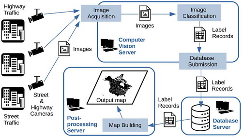
Image Acquisition: The first stage is the acquisition of the input images on which we perform the road condition classifications. These images are snapshots taken by street and highway cameras located across Canada and the United States. They are downloaded over the internet by sending snapshot queries to public camera APIs. For this task, we rely on a pre-assembled catalog containing a unique camera identifier, the snapshot URL and the geographic location for each camera of interest. As the images are downloaded periodically to the computer vision server, they are passed along to the classification module for further processing. The speed of this module is practically bound to the network bandwidth and it can be executed in multiple threads.

Image Classification: This is the core module performing the machine learning tasks. It contains the deep learning classifier with pre-trained weights. This module monitors the set of incoming images and checks them for corruption and integrity. If they are good, they are resized to the expected input dimensions of the classifier and fed into it in batches. The output is written into a catalog of label records on the local disk in form of camera identifiers, time stamps, inferred label and the geographic location tags.

Database Submission: Database Submission module monitors the label records generated by the image classification module. As they come in, they are retrieved and sent to a remote database server for further processing. This module is decoupled from the image classification task to avoid any delays.

Map Building: This module monitors the database for emerging records and fetches them to maintain an output map on which icons indicating the road conditions are superimposed on their respective geo-locations, for visual representation.

Operational Deep Learning Frameworks

In this work, we considered a variety of deep learning frameworks. We now present a brief overview of the various architectures used in this paper.

Visual Geometry Group – VGG: Developed by Simonyan and Zisserman (Simonyan and Zisserman 2014), VGG was the runner-up at the ILSVRC 2014 (ImageNet Large Scale Visual Recognition Competition). It is one of the earliest networks which showed that small convolutional filters with a deeply layered architecture can produce successful results. VGG has a deep feed-forward architecture with no residual connections. This is formed by linearly connected convolutional layers with max-pooling after every second or third layer, with two fully-connected hidden layers with optional dropouts in between, and a softmax layer at the end. This architecture was chosen for a number of reasons: i) demonstrable success on a variety of image classification tasks, ii) has a feed-forward architecture with no residual connections which makes it a good baseline, iii) has native support in Keras⁵ and its model with weights are publicly available, and iv) was computationally feasible. VGG has different flavors but a popular one, which has 13 convolutional and pooling layers and 3 fully connected layers, is called VGG-16. We used its Tensorflow implementation with Keras. We took the original VGG-16 classifier with 1000 classes, discarded the final fully-connected layer and appended a new one with 2 neurons activated via the softmax function. We used the default ImageNet weights. We set every layer non-trainable except the final one. Its second-to-last layer is fully connected with 4096 neurons which means we ended up with 4096 × 2 (weights) + 2 (bias) = 8194 trainable parameters. All the previous 134,260,544 parameters were left frozen. This baseline configuration was used in the two-class experiments discussed in Section 3.1. Its multi-class variants are also examined across the rest of Section 3, and its performance is benchmarked in Section 4.

Residual Neural Network- ResNet: Developed by Kaiming He et al. He2016, the ResNet architecture introduced a solution to the network depth-accuracy degradation problem. This is done by deploying shortcut connections between one or more layers of convolutional blocks that perform identity mapping, which are called residual connections. This allows the construction of a deeper network that is easier to optimize, compared to a counterpart deep network based on unreferenced mapping. ResNet won first place in the ILSVRC 2015 classification competition. For this work, a 178-layer deep version of ResNet50 is customized for our classification experiments. The last fully connected layer is removed and replaced by a drop-out layer followed by a fully connected layer. This architecture uses residual connections to tie non-adjacent layers with the intent of coping with vanishing/exploding gradients during the training process. We started with ResNet-50, a fifty layer deep version of this architecture. As with VGG, we used Keras with Tensorflow. We took the original classifier and configured the end layers for our 2-class problem. The final layer had 2 neurons activated via the softmax function. It’s second-to-last layer was fully connected with 2048 neurons so there were 2048 × 2 (weights) + 2 (bias) = 4098 trainable parameters. All previous layers with 23,587,712 parameters were set to non-trainable. This configuration was used in the two-class experiments discussed in Section 3.1. Its five-class variant was also examined for benchmarking purposes, discussed in Section 4.

InceptionResNetV2: InceptionResNetV2 is an integration of residual connections into the deep inception network (Szegedy et al. 2017). The model achieved lower error with top-1 and top-5 error rates compared to batch normalization-Inception, Inception-v3, Inception-Resnet-v1 and Inception-v4. In our experiments: i) the input images were rescaled to $299\times 299\times 3$, ii) the top layer was removed and replaced by a dropout layer with dropout rate of 0.4, and iii) with a softmax fully connected layer for the 5 classes. We used this framework for our five-class experiments discussed in Section 3.4 and for benchmarking, discussed in Section 4.

Extreme Inception – Xception: The Xception network was introduced by Francois Chollet (Chollet 2017) where Inception modules were replaced by depthwise separable convolutions with residual connections. In the Xception architecture, the data goes through an entry flow, then a middle flow and finally an exit flow. This process is repeated eight times. To adapt this network for our task: i) we removed the top layers and replaced them with a dropout layer, and ii) replaced the fully connected layer with softmax for the 5 classes of road conditions. We examined this framework for benchmarking, in Section 4.

EfficientNet: EfficientNet, developed by Mingxing Tan and Quoc V. Le (Tan and Le 2019), introduced a compound scaling method to scale up all three ConvNets dimensions, namely, width, depth and resolution, to achieve more accuracy and efficiency. For this work, we used the baseline models EfficientNet-B0 and EfficientNet-B4. In order to apply transfer learning, we replaced the top layer with a dropout layer followed by a softmax fully-connected layer for the 5 classes. EfficientNet-B4 is a scaled-up version of the baseline network EfficientNet-B0 by using user-specified coefficient $\varphi$ and constants $\alpha$, $\beta$, $\gamma$, which are found by grid search. The latter network width, depth and resolution are determined by ${\alpha }^{\varphi }$, ${\beta }^{\varphi }$ and ${\gamma }^{\varphi }$, respectively, under constraint of $\alpha \ast {\beta }^2\ast {\gamma }^2\approx 2$. We used this framework for our five-class experiments discussed in Section 3.4 and for benchmarking, which we discuss in Section 4.

Dataset Labeling

A major part of this work was data labeling, given that our archive contained millions of images. The archived raw images had various road and weather conditions, a variety of scenery (urban, rural), differing sky conditions (clear, overcast), and illumination (day, night, twilight). These images had to be labeled accurately and be of sufficient quality to produce a reliable set of training images (shown in Figure 1). Another challenge was to take into account model complexity and memory usage, in addition to classification accuracy during the various stages of the dataset labeling and classification process.

The overall process used to label images is summarized in Figure 3. Due to the very large size of our image archive, we first looked for an alternative to manual labeling images. Our first attempt at automated labeling was to try using road condition observations from RWIS that were located near cameras. The RWIS data from departments of transportation (DOT) across North America are transmitted to the Meteorological Assimilation Data Ingest System (MADIS).⁶ From MADIS, we retrieved RWIS road condition observations that were located within 10 km of the camera and measured within 15 minutes of the image time. Many cameras were not close enough to an RWIS for thisFigure 4 technique to work, but nevertheless, it could reduce manual effort in numerous cases. Table 1 summarizes the classes of images labeled using RWIS observations.

Figure 3. An overview of the data preparation and experimentation phases

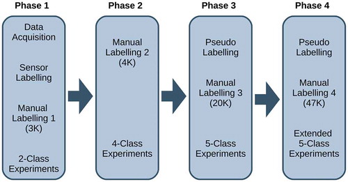
Figure 4. Augmented data samples

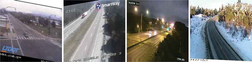
Table 1. Labeling of images by road condition sensors located near the cameras

Road Condition Id	Title	# Images	Content (Inferred Visually)
1	Dry	28,709	Mostly dry, some wet, snow
2	Moist	3,546	Mostly damp or wet, some dry
3	Moist (treated)	954	Mostly damp or wet, some dry
4	Wet	5,216	Mostly wet, some slush,snow, dry
5	Wet (treated)	584	Mostly wet, some slush, snow, dry
6	Ice	1,545	Wet, some snow, slush, dry
7	Frost	29	Seemingly dry
8	Snow	1,718	Mostly snow, some dry, wet
15	Dew	737	Mostly wet, some rainy, some dry
16	Black ice warning	66	Seemingly dry
18	Slush	2	N/A
21	Unknown	236	Wet snowflakes on road
22	Unknown	38	Light snowflakes on road
23	Unknown	149	Mostly heavier snow or slush
24	Unknown	48	Seemingly assorted

As shown in Table 1, the automated labeling using RWIS observations resulted in the dry label being assigned the vast majority of the time. While dry road conditions are likely most prevalent, we wanted our training set to include more images from the other categories. To improve the population of the non-dry categories along with the dry category, we used a form of pseudo-labeling. This concept was introduced in (Lee 2013) and it involves training a model with available labeled data and then using the model to create intermediate labels (i.e. pseudo-labels) for the unlabeled images, with their maximum predicted probability. Typically, the pseudo-labeled data is then regularized and used to fine-tune or re-train the original model. However, these methods are subject to confirmation bias and incorrect pseudo-labels may cascade and lead to a flawed classifier (Arazo et al. 2019). To ensure our composed labeled sets are reliable, we opted for inspecting the pseudo-labeled images and manually cherry-picking the results (i.e. selectively extracting the images which appeared to be correctly labeled for their respective classes from a human evaluator’s perspective). The specifics are discussed further in each experiment.

• Metrics used in this paper: The following classical metrics were used in this work:Precision, Recall and FI and Accuracy. We also keep track of Support i.e. the number of images against which these metrics are measured, and Macro Average i.e. the arithmetic mean for each metrics. In the problem we consider, our main objective is to maximize the overall accuracy of the classifier. However, we also need to measure and optimize the performance of individual classes. This is the reason behind selecting these metrics. Precision and recall reveal the bias of the classifier for each class. They are also semantically complementary. Precision reveals how many of the selected items are relevant. Recall indicates how many of the relevant items are selected. So, avoiding low precision and low recall will minimize false positives and false negatives, respectively. F1 score is the harmonic mean of precision and recall, so maximizing it will optimize both metrics, in combination. Macro averages will reveal how these metrics will reflect overall, when all classes are considered so measuring and maximizing them will also be aligned with our objective.

Experiments and Data Development

In this section, we examine the experiments and the data set development process using a multi-phased approach as shown in Figure 3. The reason behind opting for such an approach is associated with the tasks we needed to perform. These tasks included collecting data for training and experimentation, testing the feasibility of potential DCNN and transfer learning solutions, determining the labels, extracting reliable labeled data from a massive set of raw images, and deciding which frameworks (networks) to use. The lack of knowledge and insight on the data was a major roadblock to carry out these tasks. Understanding the data set better was crucial to define and populate more suitable labels for training and experimentation. Correspondingly, having more data with reliable labels would allow us to build better performing models, which could in turn be used to further improve the data set so we could develop an optimal classifier. Accordingly, the tasks in this section were accomplished in an evolving configuration where the data labeling took place along with the experimental phases and as such, the developments and findings in each phase dictated the subsequent steps. Essentially, we treated each phase as an intermediate step toward creating a reasonable data set and developing a production-level deep learning classifier to be used in the real application domain. The conditions, roles and relationships of the phases are summarized as follows:

Phase 1: We put together a small set of labeled data set and we tested the feasibility of the project as a binary classification problem. We identified a promising framework and discussed the results.

Phase 2: We doubled the number of classes and modestly increased the data set size. We retrained the model from Phase 1 and discussed the results.

Phase 3: We introduced another class to capture the dark and poor quality images. We employed the data and the model from Phase 2 to generate “pseudo-labels” for an additional set of unlabeled data. Then, we manually examined them and cherry-picked the reliable samples to update our labeled data set.

Phase 4: We finalized our data set by making each class more diverse in terms of quality so it scales better to the production environment. At this stage, we used the data set from Phase 3 and trained a classifier to create additional pseudo-labels. Then we incorporated non-cherry-picked (low quality) images and formed the final set.

The final data set was used in Section 4 to provide an ultimate analysis of the frameworks of interest, and to train the classifiers that can be used in the production environment. In that regard, the experiments in this section are provisional and they provide a precursor to what comes in Section 4, where we present a comparative accuracy and efficiency analysis for the state-of-the-art DCNNs we considered for deploying into our engineering application. We opted to de-couple these final results because we wanted to abstract them from the rest of the experiments throughout the data labeling process, as they are less relevant to data development and more relevant to the real-world application.

We used heuristics to select which frameworks (networks) to examine and work with in this section. Depending on the phase, we had one of two concerns in mind. Early on, our hardware was limited and thus we examined and worked with ResNet and VGG which were sufficiently lightweight to be used for our purposes. These networks allowed us to quickly tweak hyper-parameters and perform preliminary experiments. In the later stages of this project, with a hardware upgrade, we were able to try more recent and advanced architectures. We observed significant performance gains, particularly with InceptionResNetV2 and EfficientNet-B4. After our hardware upgrade, we also had the chance to consider XCeption and EfficientNet-B0 for the phases described in Section 3.

Phase 1 – The Two-Class Problem

Introduction

In this phase, the goal was to prepare a two-class balanced training set (dry and non-dry) based on 352,240 unlabeled images that had been collected across North America using the method described in Section 2.1. Particularly, we considered the subset of images with RWIS data shown in Table 1. Using the observations from RWIS, only 10–20% of the samples could be verified and labeled, so useful samples had to be cherry-picked. Furthermore, as shown in Table 1, many of the classes were under-sampled and therefore unusable in their initial form. To address this, classes were merged together under the generic non-dry class. By doing some cherry-picking on categories 1, 4, 5, 6, 7, 8, 16, 18, 21, 22, 23, 24 we extracted 1785 assorted non-dry samples consisting of wet, snowy, slushy and icy images. After that, we matched this class with an equal number of dry samples. Finding dry images was easy since they were abundant. Both classes span a variety of scenery (urban, rural), sky conditions (clear, overcast), illumination (day, night, twilight) and quality. We randomly split the data into training and validation sets for two classes, each of which we reserved 1585 samples for training and 200 samples for validation.

Two-Class Experiments on 3 K Data Set

For both VGG-16 and ResNet50, we used a batch size of 10 and we trained both networks for 20 epochs with increments of five using our 3170 training samples. Then we tested the models on our 400 validation samples. Their respective classification metrics and confusion matrices are presented in Table 2.

Table 2. Phase 1 classification metrics and the confusion matrix for ResNet-50 (top) and VGG-16 (bottom) frameworks

		ResNet-50
		Classification Metrics
	Precision	Recall	F1-Score	Support	Accuracy
Dry	0.61	0.97	0.75	200
Non-dry	0.91	0.38	0.53	200
Macro Avg.	0.76	0.67	0.64	400
Training					88.7%
Validation					67.0%
		Confusion Matrix
	True\Predicted	Dry	Non-dry
	Dry	193	7
	Non-dry	125	75
		VGG-16
		Classification Metrics
	Precision	Recall	F1-Score	Support	Accuracy
Dry	0.79	0.88	0.83	200
Non-dry	0.86	0.77	0.81	200
Macro Avg.	0.83	0.82	0.82	400
Training					94.0%
Validation					82.3%
		Confusion Matrix
	True\Predicted	Dry	Non-dry
	Dry	176	24
	Non-dry	47	153

Analysis

Based on our experiments in Phase 1, it can be seen that the classifiers have been able to differentiate between dry and non-dry images, showing promise for the upcoming multi-label classification tasks. Also, VGG-16 outperformed ResNet-50 in terms of overall accuracy and F1 scores. This is due to the lopsided recall performance of ResNet-50, yielding a heavy bias toward the dry class. The macro averages for ResNet-50 across the metrics were poorer, in spite of the fact that ResNet-50 has a higher non-dry precision than VGG-16.

It is also interesting to note that both frameworks exhibited similar tendencies, with higher recall for dry and high precision for non-dry. This is presumably due to the fact that the dry class had higher intra-class similarity, making it easier to capture and recall its defining features. On the contrary, the non-dry class spanned a wider range of conditions, resulting in a higher intra-class variation. The features of this class were captured as far as the limited training samples allowed to do so, leading to higher precision values but relatively lower recall values for the non-dry class.

The main importance of these results is that they showed we can employ modern DCNN frameworks along with transfer learning to achieve non-trivial results. Another interesting thing to note is that these results were achieved without performing any pre-processing on the images (noise removal, text/logo removal, histogram equalization, cropping etc.), other than rescaling. This suggests that modern architectures have the potential to adapt to our scene classification problem. We should also note that throughout the first round of data labeling and experimentation, we identified a number of potential challenges for interpreting the image content which would also be relevant to future experiments. They include: i) Resolution: Images had varying resolutions and aspect ratios. The majority were 320 by 240 but they ranged from 160 by 90 to 2048 by 1536. Modern CNN architectures expect inputs of uniform size so they would have to be resized accordingly. This means the solution we develop would need to be scale-invariant, ii) Illumination: Depending on the time of the day, some images yielded very dark scenes, making it practically impossible to judge the road condition, iii) Corruption: We came across some corrupted images containing regions with pixelation and unnatural colors, iv) Occlusion: Certain images had objects partly or fully blocking the view, v) Superimposed Texts: Most images contained a superimposed logo and text on the camera view. These would have to be sampled adequately across the classes to prevent our model from using them as features, vi) Varying Angles: The angle at which the cameras view the road varies greatly. Some cameras have top-down views, others are almost at eye-level, vii) Varying Distance: The distance between the cameras and the roads vary widely, viii) Imbalanced Categories: The vast majority of the images were the ideal dry condition. Conditions like snow, slush and ice seemed significantly less frequent, ix) Offline Cameras: From time to time, cameras show a “stream offline” message rather than the actual video feed. Based on the promising results we achieved with VGG-16 on a simplified two-class configuration, we decided to use the VGG-16 architecture to expand the task to a multi-label (4-class) classification problem.

Phase 2 – The Four-Class Problem

Introduction

The natural way to convert this into a multi-label problem was to decompose the non-dry class into its constituents. However, the subclasses were very imbalanced in terms of size with some have a negligible number of images. Therefore, the non-dry subclasses broadly categorized under two streams of equal size (1785 images): “wet” and “snow.” In addition, there were also thousands of snapshots with the aforementioned offline message. These images with offline messages were on cameras where the video stream was not available. Since these images would also be present in the production environment it was important to capture and filter such images. In total, 677 offline images were extracted. The classification task in this phase then used the following classes: i) Dry: This class represented seemingly ideal dry conditions during the day or night, ii) Wet: This class represented a spectrum of conditions from moist roads to puddles to soaking wet., iii) Snow: This class represented harsh winter conditions including snow-covered, slush-covered, and ice-covered roads, iv) Offline: This class covered the no-signal feed from offline camera images.

The new data set is composed of 1785 Dry, 880 Wet, 905 Snow and 677 Offline images. For each class we reserved 20% of samples for validation. At this stage, we used mostly dry images because we wanted to observe the behavior of the classifier over an unevenly distributed data set reflecting the composition of the 352 K data set, which better resembled the distribution of the real-time production environment.

Four-Class Experiments on 4 K Data Set

For this stage, we decided to repurpose the VGG-16 classifier from Section 3.1 since it showed more promise. We essentially employed the same hyper-parameters as Section 3.1 except that we changed the final layer to include 4 neurons for our four-class setup. We split the labeled data as 95% training and 5% validation. We reserved a smaller portion for validation since we had more classes with fewer images. After training a VGG-16 classifier for 5 epochs, the training set accuracy was 83.5% and the validation set accuracy was 77.1%. The classification metrics and the confusion matrix for the validation set are presented in Table 3.

Table 3. Phase 2 classification metrics and the confusion matrix for VGG-16 framework

		VGG-16
		Classification Metrics
	Precision	Recall	F1-Score	Support	Accuracy
Dry	0.81	0.78	0.79	89
Offline	0.97	1.00	0.99	33
Snow	0.83	0.78	0.80	45
Wet	0.51	0.58	0.54	43
Macro Avg.	0.78	0.78	0.78	210
Training					83.5%
Validation					77.1%
		Confusion Matrix
True\Predicted	Dry	Offline	Snow	Wet
Dry	69	0	2	18
Offline	0	33	0	0
Snow	3	1	35	6
Wet	13	0	5	25

Analysis

This round of experimentation resulted in a mixed set of results. The overall accuracy decreased to 77%, although this was still promising since we had twice as many labels and the decomposed wet and snow classes had effectively half as many samples to work with. A detailed class-based analysis is presented below:

Dry: Dry performed slightly worse than the two-class experiment, mainly due to the fact that the model had difficulty distinguishing between the dry and the wet classes. These classes seemed to have relatively higher inter-class similarity. More training samples were necessary.

Wet: This class suffered more than the dry class mainly because of its smaller size. We think when these samples were represented together with the snow class, they were easier to tell apart from the dry images because wet and snow actually have many common features such as less visibility and more frequent overcast scenes. These features did not appear to be emphasized as much by the model since they are now associated with multiple classes.

Snow: This class offered similar results to the two-class experiments, which is impressive considering the fact that it had effectively half as many examples as in Section 3.1. This is most likely because the snow class had more distinctive features compared to the dry and wet classes, such as the color and the texture of the road being much different.

Offline: The classifier performed exceptionally well (with 100% accuracy) over the new offline category. We think this is because of its distinctive features such as large texts and unnatural colors, which are totally different from a regular road scene.

One important observation is that there is a smaller margin between the precision and recall values – for any given class – compared to the previous phase. We see a more balanced outcome for these metrics. This suggests that the model exhibits less bias toward the dry class. This is also reflected in the macro averages, as they yield similar values for all three metrics. Although the F1 scores vary significantly across the classes, and the room for improvement – especially for the wet class – remains, such low precision-recall gaps suggest the classifier is improving and fitting the data better than the previous phase, even though there are more classes to learn.

Overall, the experiments showed that VGG-16 was still able to show a decent performance on a four-class setup, even with a small subset of images that had an uneven training data distribution. Validation results suggest that the highest degree of confusion was between dry and wet categories, whereas the number of mistakes among the other pairs was smaller. Remarkably, the model was exceptionally good at classifying offline images. In the next phase, we explored the ways to increase the size of our labeled data set.

Phase 3 – The Five-Class Problem

Pseudo-Labeling with VGG

In Phase 3, the goal was to leverage the VGG-16 classifier trained on the four-class experiments and use a semi-supervised learning method on the large 352 K data set to “pseudo-label” each image with one of our four classes. This approach was used to assist us in clustering images of similar nature, making the manual cherry-picking stage much easier. We incorporated our 4-class model from Section 3.2 (after retraining it via 95%-5% training-validation split) to classify 352,240 images which took under a day on an Intel i7 3630QM machine with 16GB system RAM and a NVIDIA GeForce 670MX GPU with 3GB video RAM. The number of pseudo-labels suggested per class by VGG-16 were as follows: 142,413 Dry, 99,089 Wet, 70,200 Snow and 40,538 Offline.

At this stage, we were not able to use concrete metrics for the classification accuracy over the 352 K set as they were mostly unlabeled data. However, as we examined the thumbnails, we observed similar types of classification errors as in previous experiments on the validation set. Dry and wet samples were being identified incorrectly on dark and overcast imagery, dry winter samples were sometimes getting mistaken for snow, but we were still seeing exceptionally good results for the offline class. An overview of the extracted content by means of semi-supervised learning is presented below:

Dry: This label congregated mostly clear-sky images and well-lit scenes with dry and clean pavements. Daytime and summer-looking images from lower latitude regions appeared frequently whereas winter and night images were sparse. We observed occasional false positives under this label including images with wet/moist roads and, to a much lesser degree, snowy roads. There were only a handful of offline images. Compared to the false positives, there were more false negatives. We noticed that many dry road images featuring dirty roads, overcast skies, night scenes, and dark pavements appeared under the “wet” label. Likewise, some winter images with dry roads appeared under the “snow” label.

Wet: This label accumulated a lot of rainy and wet surface images. In addition, a significant portion of the images were overcast dry, fuzzy, foggy, blurry, dark and night scenery, dirty or otherwise unintelligible scenes which were not necessarily wet. Infrequent snow and wet-snow images were present. Offline samples were again negligible. Overall, we came across many false positives and false negatives for this label but there were sufficient true positives with wet roads to be harvested for our purposes.

Snow: For this class, we observed less frequent false negatives compared to the other labels. However, there were many false positives. Wet and dry images were frequently present, and although most of them were winter scenes with snowy backgrounds, the roads were clear. As with the “wet” category, we observed fuzzy, blurry, foggy, dark, and night scenery. There were also dirty or otherwise illegible scenes (not necessarily snowy). There were a negligible number of offline images.

Offline: This was by far the most accurate label. False negatives were negligible and false positives were very sparse. It seemingly encapsulated the vast majority of the offline imagery along with some almost-black pictures. At this stage, the model seemed to have learned the offline patterns that it had not been trained on and even though we used a small number of training samples for this class, it was able to generalize very well over the unlabeled data.

Manual Labeling

Training a 4-class VGG-16 network and running it on the entire 352 K data set helped us cluster similar images and significantly narrow down sets of potentially interesting images for each class. We were able to manually label 9620 Dry, 5012 Wet and 4028 Snow samples. During this phase, we observed that a huge portion of poorly-lit night images ended up in either snow or wet categories. These images (1108) were very hard to label even by human classifiers and hence led to a new category “poor.” The description of the fifth class is as follows:

Poor: This class contains images that a human was unable to classify, due to various factors including: darkness, poor visibility, blurriness, or uncertainty about the category (e.g. wet vs. ice).

Including 676 Offline images, the total number of samples in this round were 20,444. Once again we used 20% of the images for validation.

Five-Class Experiments on 20 K Data Set

For this round of experimentation, we decided to retrain the VGG-16 classifier for two reasons. Firstly, because we had a more substantial number of samples for training and we wanted to allow more layers to be tuned. In order to increase the fitting capacity of the model, we planned to train all the fully connected layers along with the last few convolutional layers. However, we came across over a hundred million parameters to be tuned, which our hardware could not handle. Therefore, we needed to reduce the number of parameters by shrinking the fully connected layers. The standard form of VGG-16 contained 4096 neurons per hidden layer which was reduced to 1024. Secondly, we realized we could further diversify our data set and hopefully improve the performance with data augmentation. This technique introduces additional training samples to the data set by transforming and deforming the originals (randomly shifting, rotating, zooming, flipping etc.) as shown in Figure 3. Although new samples would be correlated with the original images, they could counteract over-fitting in some cases as the transformations and deformations challenge the training process.

We used an 80–20 split and trained this VGG-16 classifier initialized with ImageNet⁷ weights. The results are presented in Table 4.

Table 4. Phase 3 classification metrics and the confusion matrix for VGG-16 framework

		VGG-16
		Classification Metrics
	Precision	Recall	F1-Score	Support	Accuracy
Dry	0.88	0.93	0.90	1924
Offline	1.00	0.98	0.99	136
Poor	0.91	0.91	0.91	222
Snow	0.92	0.91	0.91	806
Wet	0.87	0.79	0.83	1003
Macro Avg.	0.92	0.90	0.91	4091
Training					94.1%
Validation					89.0%
	Confusion Matrix
True\Predicted	Dry	Offline	Poor	Snow	Wet
Dry	1780	0	6	41	97
Offline	0	133	3	0	0
Poor	9	0	202	5	6
Snow	55	0	1	733	17
Wet	181	0	9	19	794

Analysis

Experiments in this phase yielded the best results yet. The F1 scores for dry, wet, and snow all increased as we quadrupled our labeled data set and incorporated data augmentation. The new “poor” class also performed well, achieving an F1 score of 91%. The most challenging task was still distinguishing dry and wet images, although it should be noted that we saw a big improvement in the F1 score for the wet class from 54% to 83% with the additional samples.

Precision and recall values keep improving consistently across the classes, and this also reflects on the F1 scores and the macro averages. The biggest improvement has been observed in wet class precision, suggesting that additional samples introduced at this stage allowed the model to extract more reliable features. Nonetheless, room for improvement remains for the recall metric for the wet class, as there is still some bias toward the dry class.

Another point worth mentioning is that at the end of this phase, we achieved the lowest deviation so far, between the peak validation accuracy and the underlying training accuracy. This suggests that over-fitting became less of a concern at this point and we got a better representation of the images in our model, extending its performance on the training set to the validation set relatively well. It should be observed that this result was obtained with a cherry-picked manually labeled 20 K dataset.

Up to this point, we exclusively worked on the 352 K images that had been collected prior to this project. Although it may seem like a set of decent size for experimentation and training set formation, the fact that an overwhelming majority of the images were from dry roads and poor/night scenery left us little data to work with. Accordingly, we used the mean time to acquire additional road camera samples beyond our 352 K data set. An extra 1.1 million images were collected using the same method described in Section 2.1. Combined with our earlier unlabeled images, we were able to generate a 1.5 million-image data set.

We extracted 1000 images randomly and we let our VGG-16 model classify this set. Then we manually interpreted the results. Taking into account the ambiguous and fuzzy cases which could belong to multiple labels, we marked each result as “acceptable” which were most likely (or at least partially) correct or “refused” which were absolute false positives. Table 5 shows these results where the overall classification accuracy was good (88%) for the dry, offline and poor classes. However, the performance on wet and snow categories was unacceptable. There were too many false-positives. Upon further examination, we realized most of them were poor images incorrectly assigned to these classes. Therefore, we decided that our training set would need to be diversified with more low-quality samples.

Table 5. Classification judgment for 1000 random images from combined (1.5 M) data sets

# Images	Verdict	Dry	Offline	Poor	Snow	Wet	Total
VGG-16	Acceptable:	616	65	136	9	62	888
20 K	Refused:	31	0	7	21	53	112

Phase 4 – Scaling the Solution

Second Pseudo-Labeling

In this phase, we decided to perform another round of labeling using semi-supervised learning as in Section 3.2. This time, we applied our five-label VGG-16 classifier trained in Section 3.3 with 89% validation accuracy on both the 352 K data set and the 1.1 M data set. Table 6 shows the number of images pseudo-labeled by class.

Table 6. VGG-16 pseudo-labeling results the 352 K and 1.1 M data sets

VGG-89%	352 K Set		1.1 M Set
Pseudo-Labels	# Images	%	# Images	%
Dry	216,614	61.50	748,165	67.16
Poor	49,707	14.11	143,016	12.84
Wet	43,479	12.34	114,700	10.30
Offline	26,827	7.62	91,163	8.18
Snow	15,613	4.43	16,876	1.52
Total	352,240	100.00	1,113,920	100.00

For the 352 K data set, the number of dry samples increased whereas the others decreased. This seemed to be a step in the right direction since many of the poor samples already migrated to the poor class after it was introduced. Also, in Section 3.2 those classes were suffering from low precision, so having fewer samples appear in those categories was a good sign, suggesting less false positives and a higher precision. In the 1.1 M data set, we had a similar distribution, albeit not the same. Here, the dry class samples dominated even more. Also, snow samples were especially rare since those images were captured later in spring.

Manual-Labeling

In our earlier process of generating labeled sets, we used suggestions by the VGG-16 network to cherry-pick high confidence samples and ignored the remaining majority samples which resulted in a high validation accuracy. However, we were still facing many false positives and ambiguous samples. So in this phase, we decided to have all types of images represented in our model for training and validation.

Accordingly, we considered the 1.5 million images with their pseudo-labels and we randomly extracted 4000 samples from each of the five classes. Then we manually labeled them. This time, unlike in Section 3.2, we did not cherry-pick the results. We did not discard any image, but included them in the “poor” class if we were unable to label them with confidence. So now, the poor class represented all types of problematic images including the challenging images discussed in Section 3.1.

To ensure that we did not trivialize our original high confidence cherry-picked training samples by the new randomly extracted images, we also performed another set of cherry-picking, although to a lesser degree. Overall, we supplemented our 20 K data set with 20 K randomized and 7 K cherry-picked samples, creating a new data set with 47 K images. Table 7 shows the final labeled data set.

Table 7. Final 47 K labeled data set with 5 classes

# Images	Total	Train	Validation
Dry	16,065	14,458	1607
Offline	5225	4702	523
Poor	9259	8333	926
Snow	7565	6808	757
Wet	9228	8305	923
Overall	47,342	42,606	4736

Five-Class Experiments on 47 K Data Set

At this stage of the project, we upgraded our development machine to an Intel i7 9700 K CPU with 32GB RAM and an NVIDIA GeForce RTX 2080 GPU with 8GB Video RAM. This enabled us to experiment with more advanced frameworks such as InceptionResNetV2 and EfficientNet-B4 in addition to VGG-16. InceptionResNetV2 is a very deep and sophisticated architecture with 55 million parameters spread across 572 layers compared to the VGG-16 model with 48 million parameters over 23 layers (including non-convolutional layers). Introduced recently by Google AI, EfficientNet leverages scalability in multiple dimensions, unlike most other networks. It employs 18 M parameters. For all three frameworks, we used our 47 K data set with a 90–10 training/validation split and data augmentation to maximize the training samples. As we multiplied the size of our data set, this ratio yielded a similar number of validation examples as Section 3.3. We now give the results of experiments with the three frameworks.

VGG-16: It was trained with our previous hyper-parameters except that we used 1280 neurons in the fully connected layers, which resulted in 40 million parameters to be trained. Table 8 shows the classification metrics and the confusion matrix after epoch 7.

Table 8. Phase 4 classification metrics and the confusion matrix for VGG-16 framework

		VGG-16
		Classification Metrics
	Precision	Recall	F1-Score	Support	Accuracy
Dry	0.87	0.88	0.87	1607
Offline	0.99	0.98	0.99	523
Poor	0.88	0.84	0.86	926
Snow	0.90	0.85	0.88	757
Wet	0.80	0.85	0.82	923
Macro Avg.	0.89	0.88	0.88	4736
Training					88.9%
Validation					87.3%
	Confusion Matrix
True\Predicted	Dry	Offline	Poor	Snow	Wet
Dry	1419	0	53	22	113
Offline	1	511	11	0	0
Poor	67	3	779	31	46
Snow	36	0	35	646	40
Wet	117	0	8	17	781

InceptionResNetV2: This model was trained from the original ImageNet weights with all the layers set as trainable. There were a total of 54 million parameters to be trained. There were no modifications to the original model except for the final dense (output) layer. No dropout was applied. Details are presented in Table 9.

Table 9. Phase 4 classification metrics and the confusion matrix for inceptionResNetV2 framework

		IRN-V2
		Classification Metrics
	Precision	Recall	F1-Score	Support	Accuracy
Dry	0.90	0.92	0.91	1607
Offline	0.99	0.99	0.99	523
Poor	0.88	0.87	0.88	926
Snow	0.92	0.90	0.91	757
Wet	0.88	0.88	0.88	923
Macro Avg.	0.92	0.91	0.91	4736
Training					90.8%
Validation					90.7%
		Confusion Matrix
True\Predicted	Dry	Offline	Poor	Snow	Wet
Dry	1474	0	67	11	55
Offline	1	519	3	0	0
Poor	58	4	810	18	36
Snow	25	0	30	684	18
Wet	75	0	10	30	808

EfficientNet-B4: This model was trained for 4 epochs. Leaky ReLU was used for activation. The results are shown in Table 10.

Table 10. Phase 4 classification metrics and the confusion matrix for efficientNet-B4 framework

		EN-B4
		Classification Metrics
	Precision	Recall	F1-Score	Support	Accuracy
Dry	0.90	0.92	0.91	1607
Offline	0.98	0.99	0.99	523
Poor	0.91	0.84	0.87	926
Snow	0.94	0.92	0.93	757
Wet	0.86	0.92	0.89	923
Macro Avg.	0.92	0.92	0.92	4736
Training					90.3%
Validation					90.9%
		Confusion Matrix
True\Predicted	Dry	Offline	Poor	Snow	Wet
Dry	1471	0	56	7	73
Offline	0	520	3	0	0
Poor	75	8	776	23	44
Snow	29	1	17	693	17
Wet	54	0	5	18	846

Analysis

With 87.3% validation accuracy over 5 classes, VGG-16 maintained a slightly worse validation accuracy on the 47 K set than the previous 20 K cherry-picked data set. This is noteworthy since this set was much more representative of the unlabeled data set as half of it consisted of unrestricted (non-cherry-picked) images and the other half is strictly cherry-picked images. Also, note that the gap between training and validation accuracies is less than 2% showing we are not over-fitting the training data. InceptionResNetV2 achieved an even higher accuracy. Within 4 epochs, it reached 90.7%, beating even the cherry-picked experiments of VGG-16 in Section 3.3. This model also did not suffer from over-fitting as the training accuracy was only 0.1% better than the validation accuracy. EfficientNet-B4 performed slightly better than InceptionResNetV2. After epoch 4, it achieved 90.9% validation accuracy overall, yielding the highest accuracy. It achieved the highest F1 score for wet and snow, and tied with InceptionResNetV2 for dry and poor classes.

In terms of precision and recall, VGG-16 exhibited a similar degradation as the accuracy for most classes, compared to the last phase. This is likewise due to the more challenging nature of the extended data set, as the low quality samples and the poor class itself now have a border that is fuzzier. Interestingly, the wet class suffered the least, and the precision-recall gaps reduced for both wet and dry classes, with the expense of an increased gap for poor and snow classes. This led to a smaller difference in macro average values for precision and recall, and ultimately, to a less biased classifier overall. The outcomes for InceptionResNetV2 and EfficientNet-B4 were even better. They outperformed VGG-16 in terms of absolute precision and recall values. InceptionResNetV2 yielded the smallest precision-recall gap with all metrics above 0.87, whereas EfficientNet-B4 produced the highest macro average value of 0.92 for all three metrics.

To observe their performance on the unlabeled set, we labeled the random extract with 1000 images from the 1.5 million data set, described in Section 3.4. Table 11 shows the combined results. For the frameworks trained on the 47 K data set, we can see that the number of false positives decreased across all classes. There were also significant improvements for snow and wet classes, compared to the VGG-16 classification on the cherry-picked 20 K set. Once again, EfficientNet-B4 proved to be the most accurate framework. It achieved the lowest false positives on dry, snow and wet classes. It also achieved the highest true positives on the wet class.

Table 11. Summary of classification judgments for 1000 random images from the combined (1.5 M) data set

# Images	Verdict	Dry	Offline	Poor	Snow	Wet	Total (1000)
VGG-16	Acceptable:	616	65	136	9	62	888
20 K	Refused:	31	0	7	21	53	112
VGG-16	Acceptable:	599	79	205	8	70	961
47 K	Refused:	17	0	0	1	21	39
IRN-V2	Acceptable:	587	76	247	10	54	974
47 K	Refused:	20	0	0	3	3	26
EN-B4	Acceptable:	608	78	217	9	66	978
47 K	Refused:	18	1	0	1	2	22

Training with more data, diversifying the poor class and using a higher-end classifier with more layers trained reflected on the results very positively. The number of evident false positives significantly decreased overall. In the next section, we will perform a comparative analysis of the run-time performances for multiple frameworks.

Discussion of Results and Real-time Map Building

In this section, we discuss results from the six trained deep-learning models: VGG-16, ResNet50, Xception, InceptionResNetV2, EfficientNet-B0 and EfficientNet-B4. They were trained from scratch, on the 90–10 split 47 K data set to see how they would compare as far as accuracy and execution time (training + validation) was concerned. Table 12 shows the common configurations and the hyper-parameters that were shared across the frameworks. Table 13 shows the algorithm-specific configurations that were shaped using heuristics or default/suggested values. For the first 4 algorithms, we used the official Keras implementations and applied transfer learning as usual. However, we used a third-party implementation of EfficientNet.⁸

Table 12. Common configurations

Hyper-parameter	: Value
Optimizer	: Rectified Adam
Learning Rate	: 0.0001
Loss Func.	: Categorical Crossentropy
Activation Func.	: Softmax
Global Pooling	: Average
Batch Size	: 16
Max Epochs	: 12
0–1 Rescaling	: Yes
Training Set	: 42,606
Validation Set	: 4736
Target Classes	: 5
Augmented Training	: Yes

Table 13. Algorithm-specific configurations. H: Hidden. D: Dropout

	VGG-16	RN-50	XCep.	IRN-V2	EN-B0	EN-B4
Input Dims	(224, 224)	(224, 224)	(299,299)	(299, 299)	(256, 256)	(256, 256)
Global Pooling	None	Average	Average	Average	Average	Average
Top Layers	H-D-H-D	D	D	D	D	D
FC Neurons	4096	0	0	0	0	0
Dropout Rate	0.4	0.4	0.2	0.4	0.2	0.4
Total Layers	25	178	135	783	233	470
Total Prms.	134 M	23 M	20 M	54 M	4 M	18 M
Trainable Prms	134 M	23 M	20 M	54 M	4 M	18 M
Nontrain. Prms	0	53 K	54 K	60 K	42 K	125 K

Accuracies and the execution times of these experiments can be seen in Figures 5 and 6 respectively. As far as the accuracy is concerned, we can see that VGG-16 and ResNet lag behind the XCeption and InceptionResNetV2 frameworks. In this particular set of runs, the highest observed validation accuracy was 90.6% after epoch 6 of EfficientNet-B4 (1200 ms execution time) while the others take turns to achieve the highest validation accuracy in other epochs. For the execution times, EfficientNet-B0 is the winner (600 ms execution time). It is only bested by ResNet50 (400 ms execution time) which nonetheless has poorer validation accuracy (85.67%).

Figure 5. Training accuracy (left) & validation accuracy (right) over 12 epochs for 6 algorithms

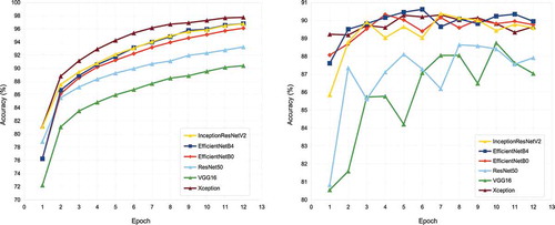
Figure 6. Execution times (training + validation + model saving) over 12 epochs for 6 algorithms. Left: Per epoch. Right: Cumulative

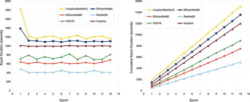
EfficientNet-B0 took about half the time of its competitors, with a validation accuracy was 90.3%, suggesting that it may be a good trade-off. Although not as accurate, VGG-16 with transfer learning proved to be very useful for data acquisition and pseudo-labeling with limited hardware resources, throughout this project. However, more recent frameworks like XCeption, InceptionResNetV2 and EfficientNet performed better, provided that the hardware to handle them is available.

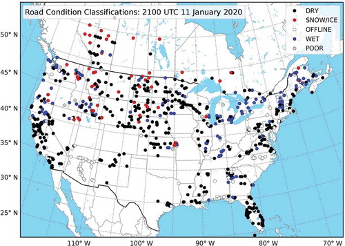
Once all images in the pipeline have been classified, the data is stored in csv files and can also be uploaded to a PostgreSQL database, if desired. These output data contain the image name, latitude and longitude, and class. A map plotting program then takes the data and produces a map for the desired domain. An example output map for all of North America is shown in Figure 7 with 782 classified images using the EfficientNetB4 framework. For this particular set of images, we observed 96.7% classification accuracy, which is mostly in-line with our observations on the 47 K data set. Details are summarized in Table 14.

Table 14. Classification judgment for the 782 images captured real-time in Canada and the United States at 2100 UTC 11 January 2020

# Images	Verdict	Dry	Offline	Poor	Snow	Wet	Total (782)
EN-B4	Acceptable:	432	109	24	55	136	756
Live Images	Refused:	20	0	0	1	5	26
Accuracy							96.7%

Figure 7. An example map of 782 classified camera images over Canada and the United States at 2100 UTC 11 January 2020. Each marker represents one classified image with the legend indicating the color corresponding to each respective class

Imbalanced data set was one of the challenging aspects of this project. For the real-world samples which we used to create our labeled data sets, the vast majority were dry and poor/night, so it was a difficult task to create a representative labeled set for training and experimentation. To deal with this problem, we relied on heuristics and experimental observations. Mainly, we used two methods to cope with the issue of imbalance. The first one was selective sampling: we initially focused on and extracted samples for the minority (non-dry) classes and later proceeded with the majority (dry). As such, the non-dry images were over-sampled whereas the dry ones were under-sampled, creating a more balanced set than we would otherwise have. Later on, we employed data augmentation. This way, we vastly enlarged and diversified the training set, and this was especially helpful for the minority classes.

Our strategies were also affected by the conditions and objectives of the particular phases. In the early phase, we opted for a perfectly balanced set to examine the potential of the prospective algorithms and the feasibility of this project. Later on, we used a skewed data set toward the dry class to provide a better approximation to the real world. Note that even in the final data set, minority classes were significantly over-sampled as the difference in the real world is even bigger. However, this skew offered a balance between the ideal theoretical conditions and the application domain.

Arguably, an imbalanced set poses the risk of over-fitting for the majority classes (and under-fitting for the minority classes), however, this risk reduces as the data set grows and the training is supported with data augmentation/regularization. This is indeed consistent with our experiments as we advanced to the final phase, the precision, recall and F1 metrics values of all classes approached to the same level, and our overall accuracy increased, despite having a skewed data set.

Conclusion

In this paper, we have presented a detailed account of the process for generating training examples from live camera feeds depicting a wide range of road and weather conditions in Canada and the United States. Our process involved leveraging deep convolutional neural networks in conjunction with manual labeling to produce reasonable quality training examples. The proposed application pipeline includes a map building component which is one of the main outcomes of this research. We demonstrated that recent deep convolutional neural networks were able to produce good results with a maximum accuracy of 90.9% without any pre-processing of the images. The choice of these frameworks and our analysis take into account unique requirements of real-time map building functions. Therefore, in addition to the classification accuracy, model complexity and memory usage were taken into account during the different stages of dataset labeling.

Our experiments show that with an increasing number of training examples available with more diverse content, the results tend to improve. With a sufficiently large training set, the performance of these frameworks on other benchmarks also applies well to this particular problem. Newer frameworks with higher benchmark scores in other problems also performed better (Bianco et al. 2018).

Future research directions include experimenting with other resource demanding frameworks with good potential such as NASNet-Large (Zoph et al. 2018) and EfficientNet-B7 (Tan and Le 2019) on more advanced hardware. In addition, we will consider employing ensemble learning techniques (Opitz and Maclin 1999) in order to exploit the best aspects of multiple frameworks. We plan to seek the possibilities to incorporate road detection and segmentation (Chen et al. 2019; Lyu and Huang 2018) as a preprocessing step to crop the images and focus on the road segments. This might be especially helpful on images with low visibility of the roads such as cases where the camera is located far from the road. This research will further enhance our ability to monitor hazardous road conditions.

Disclosure Statement

There is no conflict of interest with the funders.

Additional information

Funding

This research is supported by the Natural Sciences and Engineering Research Council of Canada (NSERC) Engage grant EGP 537911-18;Natural Sciences and Engineering Research Council of Canada [EGP 537911-18];

Notes

1. https://cdan.dot.gov/query, retrieved on Aug. 10, 2020.

2. https://www.h2o.ai/, retrieved on Aug. 10, 2020.

3. https://www.automl.org/, retrieved on Aug. 10, 2020.

4. https://arxiv.org/abs/2001.09947.

5. https://keras.io/, retrieved on Aug. 10, 2020.

6. https://madis.ncep.noaa.gov/sfc_notes.shtml#note17, retrieved on Aug. 10, 2020.

7. http://www.image-net.org/, retrieved on Aug. 10, 2020.

8. https://github.com/qubvel/efficientnet, retrieved on Aug. 10, 2020.

References

- Almazan, E. J., Y. Qian, and J. H. Elder. 2016. Road segmentation for classification of road weather conditions. In Computer Vision – ECCV 2016 Workshops, ed. G. Hua and H. Jégou, 96–108. Cham: Springer International Publishing.
- Amthor, M., B. Hartmann, and J. Denzler. 2015. Road condition estimation based on spatio-temporal reflection models. In J. Gall, P. Gehler, and B. Leibeed., Pattern Recognition 3–15. Cham: Springer International Publishing.
- Arazo, E., D. Ortego, P. Albert, N. E. O’Connor, and K. McGuinness. 2019. Pseudo-labeling and confirmation bias in deep semi-supervised learning, Proceedings of the 36thInternational Conference on MachineLearning, Long Beach, California, PMLR 97, 2019.
- Bianco, S., R. Cadène, L. Celona, and P. Napoletano. 2018. Benchmark analysis of representative deep neural network architectures. IEEE Access 6:64270–77. doi:10.1109/ACCESS.2018.2877890.
- Bronte, S., L. M. Bergasa, and P. F. Alcantarilla 2009. Fog detection system based on computer vision techniques. In 2009 12th International IEEE Conference on Intelligent Transportation Systems, 1–6.
- Carrillo, J., M. Crowley, G. Pan, and L. Fu 2019. Comparison of deep learning models for determining road surface condition from roadside camera images and weather data. In Transportation Association of Canada and Intelligent Transportation Systems Canada Joint Conference, 1–16.
- Chen, P., H. Hang, S. Chan, and J. Lin 2019. Dsnet: An efficient cnn for road scene segmentation. In 2019 Asia-Pacific Signal and Information Processing Association Annual Summit and Conference (APSIPA ASC), 424–32.
- Chollet, F. 2017. Xception: Deep learning with depthwise separable convolutions. In 2017 IEEE Conference on Computer Vision and Pattern Recognition (CVPR), 1800–07.
- Crevier, L.-P., and Y. Delage. 2001. METRo: A new model for Road-Condition forecasting in Canada. Journal of Applied Meteorology 40 (11):2026–37. doi:10.1175/1520-0450(2001)040<2026:MANMFR>2.0.CO;2.
- Drobot, S., A. R. S. Anderson, C. Burghardt, and P. Pisano. 2014. U.s. public preferences for weather and road condition information. Bulletin of the American Meteorological Society 95 (6):849–59. doi:10.1175/BAMS-D-12-00112.1.
- Elhoseiny, M., S. Huang, and A. M. Elgammal 2015. Weather classification with deep convolutional neural networks. In 2015 IEEE International Conference on Image Processing (ICIP), 3349–53.
- Gallen, R., A. Cord, N. Hautière, and D. Aubert 2011. Towards night fog detection through use of in- vehicle multipurpose cameras. In Proceedings of the 2011 IEEE Intelligent Vehicles Symposium (IV), 399–404.
- Hautiere, N., J.-P. Tarel, J. Lavenant, and D. Aubert. 2006. Automatic fog detection and estimation of visibility distance through use of an onboard camera. Machine Vision and Applications 17 (1):8–20. doi:10.1007/s00138-005-0011-1.
- Krizhevsky, A., I. Sutskever, and G. E. Hinton. 2012. Imagenet classification with deep convolutional neural networks. Advances in Neural Information Processing Systems 25:1097–1105.
- Kurihata, H., T. Takahashi, I. Ide, Y. Mekada, H. Murase, Y. Tamatsu, and T. Miyahara 2005. Rainy weather recognition from in-vehicle camera images for driver assistance. In IEEE Proceedings, Intelligent Vehicles Symposium, 205–10.
- Laffont, P.-Y., Z. Ren, X. Tao, C. Qian, and J. Hays. 2014. Transient attributes for high-level understanding and editing of outdoor scenes. ACM Transactions on Graphics [ 149:1–149: 11] 33 (4):. doi:10.1145/2601097.2601101.
- LeCun, Y., Y. Bengio, and G. Hinton. 2015. Deep learning. Nature 521 (7553):436. doi:10.1038/nature14539.
- Lee, D.-H. 2013. Pseudo-label: The simple and efficient semi-supervised learning method for deep neural networks. Workshop on challenges in representation learning, ICML, 3.
- Li, Q., Y. Kong, and S. M. Xia 2014. A method of weather recognition based on outdoor images. In Computer Vision Theory and Applications (VISAPP), 2014 International Conference, 510–16.
- Li, Z., Y. Jin, Y. Li, Z. Lin, and S. Wang 2018. Imbalanced adversarial learning for weather image generation and classification. In 2018 14th IEEE International Conference on Signal Processing (ICSP), 1093–97.
- Lin, D., C. Lu, H. Huang, and J. Jia. 2017. Rscm: Region selection and concurrency model for multi-class weather recognition. IEEE Transactions on Image Processing 26 (9):4154–67. doi:10.1109/TIP.2017.2695883.
- Lu, C., D. Lin, J. Jia, and C. Tang. 2017. Two-class weather classification. IEEE Transactions on Pattern Analysis and Machine Intelligence 39 (12):2510–24. doi:10.1109/TPAMI.2016.2640295.
- Lyu, Y., and X. Huang 2018. Road segmentation using CNN with GRU. arXiv preprint.
- Narasimhan, S. G., and S. K. Nayar 2003. Shedding light on the weather. In IEEE Conference on Computer Vision and Pattern Recognition (CVPR), I–I.
- Nolte, M., N. Kister, and M. Maurer 2018. Assessment of deep convolutional neural networks for road surface classification. In 2018 21st International Conference on Intelligent Transportation Systems (ITSC), 381–86.
- Omer, R., and L. Fu 2010. An automatic image recognition system for winter road surface condition classification. In 13th International IEEE Conference on Intelligent Transportation Systems, 1375–79.
- Opitz, D., and R. Maclin. 1999. Popular ensemble methods: An empirical study. Journal of Artificial Intelligence Research 11 (1):169–98. doi:10.1613/jair.614.
- Pagani, G. A., J. W. Noteboom, and W. M. F. Wauben 2018. Deep neural network approach for automatic fog detection using traffic camera images. In The 2018 WMO/CIMO Technical Conference on Meteorological and Environmental Instruments and Methods of Observation (CIMO TECO-2018), volume 132 of Instruments and Observing Methods (IOM), 15. World Meteorological Organization.
- Pan, G., L. Fu, R. Yu, and M. Muresan 2018. Winter road surface condition recognition using a pre-trained deep convolutional neural network. In Transportation Research Board 97th Annual Meeting, number 18-00838, 17.
- Pavlić, M., H. Belzner, G. Rigoll, and S. Ilić 2012. Image based fog detection in vehicles. In 2012 IEEE Intelligent Vehicles Symposium, 1132–37.
- Ramanna, S., C. Sengoz, S. Kehler, and D. Pham 2020. Near real-time map building with multi-class image set labelling and classification of road conditions using convolutional neural networks. arXiv preprint.
- Roser, M., and F. Moosmann 2008. Classification of weather situations on single color images. In IEEE Proceedings, Intelligent Vehicles Symposium, 798–803.
- Russakovsky, O., J. Deng, H. Su, J. Krause, S. Satheesh, S. Ma, Z. Huang, A. Karpathy, A. Khosla, M. Bernstein, et al. 2015. ImageNet large scale visual recognition challenge. International Journal of Computer Vision (IJCV) 115 (3):211–52. doi:10.1007/s11263-015-0816-y.
- Sass, B. H. 1997. A numerical forecasting system for the prediction of slippery roads. Journal of Applied Meteorology 36 (6):801–17. doi:10.1175/1520-0450(1997)036<0801:ANFSFT>2.0.CO;2.
- Schmidhuber, J. 2015. Deep learning in neural networks: An overview. Neural Networks 61:85–117.
- Shen, L. 2009. Photometric stereo and weather estimation using internet images. In IEEE Conference on Computer Vision and Pattern Recognition (CVPR), 1850–57.
- Simonyan, K., and A. Zisserman 2014. Very deep convolutional networks for Large-Scale image recognition. arXiv preprint.
- Song, H., Y. Chen, and Y. Gao. 2014. Weather condition recognition based on feature extraction and k-nn. In Foundations and practical applications of cognitive systems and information processing, ed. F. Sun, D. Hu, and H. Liu, 199–210. Berlin, Heidelberg: Springer Berlin Heidelberg.
- Szegedy, C., S. Ioffe, V. Vanhoucke, and A. A. Alemi 2017. Inception-v4, inception-resnet and the impact of residual connections on learning. In Proceedings of the Thirty-First AAAI Conference on Artificial Intelligence, AAAI’17, 4278–4284. AAAI Press.
- Tan, M., and Q. V. Le 2019. Efficientnet: Rethinking model scaling for convolutional neural networks. In K. Chaudhuri and R. Salakhutdinov, editors, Proceedings of the 36th International Conference on Machine Learning, ICML 2019, 9-15 June 2019, Long Beach, California, USA, volume 97 of Proceedings of Machine Learning Research, 6105–14. PMLR.
- Villarreal Guerra, J. C., Z. Khanam, S. Ehsan, R. Stolkin, and K. McDonald-Maier 2018. Weather classification: A new multi-class dataset, data augmentation approach and comprehensive evaluations of convolutional neural networks. In 2018 NASA/ESA Conference on Adaptive Hardware and Systems (AHS), 305–10.
- Yan, X., Y. Luo, and X. Zheng 2009. Weather recognition based on images captured by vision system in vehicle. In Proceedings of the 6th International Symposium on Neural Networks: Advances in Neural Networks - Part III, 390–98.
- Zhang, Z., and H. Ma 2015. Multi-class weather classification on single images. In 2015 IEEE International Conference on Image Processing (ICIP), 4396–400.
- Zhao, B., X. Li, X. Lu, and Z. Wang. 2018. A CNN-RNN architecture for multi-label weather recognition. Neurocomputing 322:47–57. doi:10.1016/j.neucom.2018.09.048.
- Zhu, Z., L. Zhuo, P. Qu, K. Zhou, and J. Zhang 2016. Extreme weather recognition using convolutional neural networks. In 2016 IEEE International Symposium on Multimedia (ISM), 621–25.
- Zoph, B., V. Vasudevan, J. Shlens, and Q. V. Le 2018. Learning transferable architectures for scalable image recognition. In 2018 IEEE/CVF Conference on Computer Vision and Pattern Recognition, 8697–710.