Enhancing the Human Health Status Prediction: The ATHLOS Project

ABSTRACT

Preventive healthcare is a crucial pillar of health as it contributes to staying healthy and having immediate treatment when needed. Mining knowledge from longitudinal studies has the potential to significantly contribute to the improvement of preventive healthcare. Unfortunately, data originated from such studies are characterized by high complexity, huge volume, and a plethora of missing values. Machine Learning, Data Mining and Data Imputation models are utilized a part of solving these challenges, respectively. Toward this direction, we focus on the development of a complete methodology for the ATHLOS Project – funded by the European Union’s Horizon 2020 Research and Innovation Program, which aims to achieve a better interpretation of the impact of aging on health.

The inherent complexity of the provided dataset lies in the fact that the project includes 15 independent European and international longitudinal studies of aging. In this work, we mainly focus on the HealthStatus (HS) score, an index that estimates the human status of health, aiming to examine the effect of various data imputation models to the prediction power of classification and regression models. Our results are promising, indicating the critical importance of data imputation in enhancing preventive medicine’s crucial role.

Introduction

We live in the “Big Data” era, which offers a great potential for revolutionizing all aspects of society, including the healthcare domain (Dash et al. 2019). The recent advancements in medical and health domains generate, with an exponentially increasing rate, several heterogeneous data types, such as medical, demographic, molecular, cellular, and so on, offering great potential for personalized healthcare (Cahan et al. 2019). Digitization in medicine and healthcare has revolutionized how various biological processes and complex diseases are interpreted since there is the possibility for analysis and knowledge extraction from large-scale data (Flitcroft, Chen, and Meyer 2020). In this direction, longitudinal studies, such as cohort studies and natural experiments, offer a platform to study more profound challenges in the biomedical and healthcare domain (Zhao et al. 2019). The predominant way to deal with the inherent data complexity is the Machine Learning frameworks (Wiens and Shenoy 2018), which allow the exploration, development, and construction of algorithms that can learn from data and produce accurate predictions (Tai et al. 2019; Zhou et al. 2017).

Meanwhile, clinical and population health research usually includes questionnaires within longitudinal studies, creating a significant challenge regarding the missing values for several apparent reasons (non-response, loss tracking, etc.) (Pedersen et al. 2017). The proper way to deal with this critical limitation is to impute the missing information, without losing the imposed data structure (Huque et al. 2018). In the recent literature several imputation methods have been proposed for longitudinal studies (De Silva et al. 2017; Huque et al. 2018; Nooraee et al. 2018; Ribeiro and Freitas 2021; Vilardell et al. 2020; Yamaguchi et al. 2020; Zhang, Golm, and Liu 2020), while it has been shown that such a preprocess step can lead to improvements in various Machine Learning tasks, such as the data classification (Jordanov, Petrov, and Petrozziello 2018). Longitudinal studies often contain categorical information, which is restricted-transition variables. This information is usually incomplete; hence, its imputation is a significant challenge (Huque et al. 2018). The difficulty lies in the fact that there is little guidance on whether these restrictions need to be accommodated when using imputation methods (De Silva et al. 2019). Nevertheless, research in this area mainly focuses on continuous data with fewer recommendations for categorical data (Stavseth, Clausen, and Røislien 2019).

A further essential challenge when dealing with longitudinal studies is the accuracy and validity of prediction models (Licher et al. 2019). Toward this perspective, we study the prediction power in classification and regression tasks utilizing various imputation methodologies. We aim is to enhance the predictability of Machine Learning tasks on a large-scale longitudinal study. Their main characteristic is a high rate of missing values and simultaneously mine new insights and knowledge for health status across the human age. For this purpose, we employ a harmonized dataset produced within the ATHLOS (Aging Trajectories of Health: Longitudinal Opportunities and Synergies, http://athlosproject.eu/) Project (EU HORIZON2020–PHC-635316), which integrates 15 independent European and international longitudinal studies of aging.

The ATHLOS Project is based on improving a critical factor in the healthcare domain, extending the healthy lifespan. Its importance lies in the fact that in the last decades a remarkable worldwide population aging due to the increase in life expectancy is observed (Passarino, De Rango, and Montesanto 2016). The healthcare demand increases along with the increasing number of elderly populations, which consists of a high cost every year for states (Liu 2020). Health status measurements are a crusial indicator that helps prevent human health near or even in the distant future (Kelly, Curran, and Caulfield 2017). Under this perspective, the ATHLOS project aims to study better the impact of aging on health by developing a new single measure of health status. The project intends to identify patterns of healthy aging trajectories and their determinants, the critical points in time when changes in trajectories are produced, and propose timely clinical and public health interventions to optimize and promote healthy aging.

Furthermore, one of the unique features of ATHLOS is a metric of health, called HealthStatus (HS), proposed in (Caballero et al. 2017). It is a novel index for human health condition calculation using an Item Response Theory (IRT) approach. This measure is based on specific characteristics that are part of the ATHLOS features list and has shown its reliability in several studies (Arokiasamy et al. 2012; Börsch-Supan et al. 2013; Ichimura, Shimizutani, and Hashimoto 2009; Koskinen 2018; Kowal et al. 2012; Leonardi et al. 2014; Luszcz et al. 2016; Park et al. 2007; Peasey et al. 2006; Prina et al. 2016; Rodríguez-Artalejo et al. 2011; Sanchez-Niubo et al. 2019; Sonnega et al. 2014; Steptoe et al. 2013; Whelan and Savva 2013; Wong, Michaels-Obregon, and Palloni 2017). The challenge that now emerges is to discover meaningful relationships between the wide range of features found across various HS studies. Efficiently predicting HS through features that have been considered unrelated or not informative and thus excluded from its designing processes would promote its expandability in further health-related studies while opening up new avenues for HS optimization.

This study focuses on strengthening the prediction power of the ATHLOS HealthStatus score in terms of classification and regression through various imputation methods. A large variety of both well-established and cutting-edge imputation and prediction methodologies were applied. Our study shows that applying different imputation methods can greatly affect the various classification and regression schemes in terms of their accuracy and robustness. By discovering the most appropriate and methodological frameworks, we attempt to offer new insights and identify a better interpretation of the impact of aging on HealthStatus. The outcomes of our study can be considered promising, completing the puzzle of the strong outcomes that have emerged from previous studies of ATHLOS (Arokiasamy et al. 2012; Börsch-Supan et al. 2013; Dimopoulos et al. 2018; Ichimura, Shimizutani, and Hashimoto 2009; Koskinen 2018; Kowal et al. 2012; Leonardi et al. 2014; Luszcz et al. 2016; Marois and Aktas 2020; Panaretos et al. 2018; Park et al. 2007; Peasey et al. 2006; Prina et al. 2016; Rodríguez-Artalejo et al. 2011; Sanchez-Niubo et al. 2019; Sonnega et al. 2014; Steptoe et al. 2013; Whelan and Savva 2013; Wong, Michaels-Obregon, and Palloni 2017).

Methods & Experiments

In this paper, five imputation methods were applied, namely the Mean Imputation (Singh and Prasad 2013), the Linear Regression (Eekhout et al. 2014), the Dual Imputation Model (Jolani, Frank, and van Buuren 2014), the Multiple Linear Regression (Azur et al. 2011), and the Vtreat method (Zumel and Mount 2016). Subsequently, the imputed matrices have been used as input to the six traditional and state-of-the-art regression and classification tools, namely the Logistic/Linear Regression (Hosmer Jr, Lemeshow and Studivant 2013; Montgomery, Peck, and Vining 2021), the $k$-Nearest Neighbors (Zhang 2016), the Random Forest (Biau and Scornet 2013), the Extreme Gradient Boosting (XGBoost) (Chen and Guestrin 2016), and two Deep Neural Network models. Details about the methodological pipeline, an overview of the algorithms, and the analysis of the experimental setup are given in the following subsections.

Data Preprocessing – Cleaning and Preparation

The ATHLOS project provides a harmonized dataset (Sanchez-Niubo et al. 2019), built upon several longitudinal studies, originated from five continents. More specifically, it contains samples coming from more than 355,000 individuals, who participated in 17 general population longitudinal studies in 38 countries. In this paper, we used 15 of these studies, namely the 10/66 Dementia Research Group Population-Based Cohort Study (Andrews and Clark 1999; Prina et al. 2016), the Australian Longitudinal Study of Aging (ALSA) (Andrews, Cheok, and Carr 1989), the Collaborative Research on Aging in Europe (COURAGE) (Leonardi et al. 2014) the ELSA (Steptoe et al. 2013), the study on Cardiovascular Health, Nutrition and Frailty in Older Adults in Spain (ENRICA) (Rodríguez-Artalejo et al. 2011), the Health, Alcohol and Psychosocial factors in Eastern Europe Study (HAPIEE) (Peasey et al. 2006), the Health 2000/2011 Survey (Koskinen 2018), the HRS (Sonnega et al. 2014), the JSTAR (Ichimura, Shimizutani, and Hashimoto 2009), the KLOSA (Park et al. 2007), the MHAS (Wong, Michaels-Obregon, and Palloni 2017)), the SAGE (Kowal et al. 2012), SHARE (Börsch-Supan et al. 2013), the Irish Longitudinal Study of Aging (TILDA) (Whelan and Savva 2013) and the Longitudinal Aging Study in India (LASI) (Arokiasamy et al. 2012).

The 15 general population longitudinal studies utilized in this work consist of 990,000 samples in total, characterized by 184 variables, of which two are considered as response variables and the rest as independent variables. Response variables are the raw and the scaled HealthStatus scores for each individual. Regarding the independent variables (please see supplementary material, sheet S1), nine variables were removed including various indexes (sheet S2). Thirteen variables were removed, including obviously depended variables that cannot be taken into account (sheet S2). Finally, six variables were removed, including information that cannot be considered within a prediction model (sheet S2).

It is worth mentioning that the 47 variables (sheet S3) that were originally used to calculate the HS score (Caballero et al. 2017) have been excluded. These features create a statistical bias regarding the HS, which is the response variable in our analysis. Keep in mind that these variables have been previously identified as more critical in defining the HS. Thus, we expect that using the rest of the variables for predicting the HS would be a challenging task which, may reveal new insights. Finally, removing the samples for which the HS metric is missing, the resulting data matrix is constituted by 770,764 samples and 107 variables.

Imputation Methods for ATHLOS Dataset

In this study, we utilized so well established as recent imputation methods for the missing values of ATHLOS dataset. Our aim was to cover a wide variation of all imputation method categories; hence, we applied the Mean Imputation Singh and Prasad (2013), the Linear Regression imputation Eekhout et al. (2014), the Dual Imputation Method (DIM), Jolani, Frank, and van Buuren (2014) the traditional Multiple Linear Regression Imputations Azur et al. (2011), and the Vtreat method Zumel and Mount (2016).

A brief analysis of the above imputation tools is provided. Mean Imputation (MI) and Linear Regression (LR) belong to the single imputation method family, having the ability to replace an unknown missing value by a single value. MI is a simple process based on the calculations of the mean value of the non-missing values for each response variable with a numerical data type. The missing values are filled with the respective mean value for each response variable. It is a relatively fast and straightforward approach, giving good results for relatively small numerical datasets. However, it exhibits various limitations, such as it does not consider the correlation among the response variables along with the data uncertainty in the imputations (Lin and Tsai 2020). In the Linear Regression (LR) imputation, the missing values are replaced with predicted values that arise from applying a linear regression model in the non-missing data. The idea behind this process is the fact that the variables tend to be correlated. Hence, the predicting values should be affected by the observed data (Eekhout et al. 2014).

On the other hand, the Dual Imputation Model (DIM) and the Multiple Linear Regression Imputation (MLR) belong to the Multiple Imputation class, where the missing values are replaced by $n$ simulated values ($n>1$), while its main assumption is that data are missing at random. The Multiple Imputation methods deal with the uncertainty about which values to impute, a major limitation of singular imputation methods. MLR imputation reduces this limitation by combining several different plausible imputed datasets. Initially, multiply imputed datasets are constructed, and then standard statistical methods are applied to fit each one. Under this perspective, the recently proposed Dual Imputation Model (DIM) (Jolani, Frank, and van Buuren 2014) approximates an offset between the data distribution of the observed and missing data. This approximation is performed by iterating over the response and imputation models, assuming that the response as the imputation model has the same predictors.

Vtreat (Zumel and Mount 2016) is a recent imputation method that differs from similar traditional tools since it considers the uncertainty in the imputations. It includes a unique strategy with respect to the type (numerical or categorical) of the response variable, creating additional variables along with the well-known dummy variable process. For a numerical response variable (regression), one dummy variable is created to address the high cardinality categorical variables, and two dummy variables are created to cope with the novel (or rare) levels found in each categorical variable of the data set. A similar procedure is followed for a categorical response variable (classification), but in this case, one dummy variable is created to cope with the novel (or rare) levels. This inherent feature enhances the knowledge discovery of ultra-noisy data. Furthermore, Vtreat is useful in the modeling process because it allows the model to re-estimate the response on systematically missing values. This property motivated us to focus our attention on it since the nature of longitudinal studies imposes the emergence of systematically missing values at a high degree.

Regarding the experimental study and for the MI method, $141$ dummy variables were created during the conversion of $66$ categorical predictor variables. Mean values from each of the $34$ remaining predictor variable values were calculated by replacing the respective missing value indexes. For the LR Imputation, $141$ dummy variables were constructed following the same process for creating the dummy variables. A simple model was created for the remaining $34$ predictor variables:

$38;\%MathTypeMTEF21+-\%feaagKart1ev2aaatCvAUfeBSjuyZL2yd9gzLbvyNv2CaerbuLwBLn\%hiov2DGi1BTfMBaeXatLxBI9gBaerbd9wDYLwzYbItLDharqqtubsr\%4rNCHbGeaGqiVu0Je9sqqrpepC0xbbL8F4rqqrFfpeea0xe9Lq-Jc9\%vqaqpepm0xbba9pwe9Q8fs0-yqaqpepae9pg0FirpepeKkFr0xfr-x\%fr-xb9adbaqaaeGaciGaaiaabeqaamaabaabaaGcbaaeaaaaaaaaa8\%qacaWGybWdamaaBaaaleaapeGaamyBaiaadMgacaWGZbGaam4CaaWd\%aeqaaOWdbiabg2da9iaadggapaWaaSbaaSqaa8qacaaIWaaapaqaba\%GcpeGaey4kaSYaaybuaeqal8aabaWdbiaadMgacqGH9aqpcaaIWaaa\%beqdpaqaa8qacqGHris5aaGccaWGHbWdamaaBaaaleaapeGaamyAaa\%WdaeqaaOWdbiaadIfapaWaaSbaaSqaa8qacaWGPbaapaqabaGcpeGa\%ey4kaSYefv3ySLgznfgDOfdaryqr1ngBPrginfgDObYtUvgaiuGacq\%WF1pG8aaa55B8X_{miss}=a_0+{\displaystyle \sum _{i=0}{a}_i}{X}_i+\in$

where $X_{miss}$ is the predictor variable, with missing values, to be imputed, $X_i$ is the list of $n$ complete predictor variables, $a_i$ are the regression coefficients, $a_0$ is the intercept, and $\epsilon$ is the normally distributed error.

Regarding the application of MLR (Multiple Linear Regression) imputation, we followed the multiple imputation main steps by using the Linear Regression model to perform the $m$ complete data analyses. Consider $X$ as the ATHLOS data matrix of the $34$ predictor variables. As $Y$ the partially observed predictor variable to be imputed, while $Y_{miss}$ indicates the missing parts of $Y$, and $R$ is the $770,764\times 33$ binary matrix indicating the elements of $X$ that are observed $\left(R_{ij}=1\right.$ if $X_{ij}$ is observed). Initially, MLR defines the posterior predictive density as $p(Y_{miss}|X,R)$. Subsequently, imputations are generated based on this density by concatenating $m=5$ complete datasets. In the next step, a Linear Regression model was applied on each completed data matrix performing $m=5$ complete data analyses, while an ensemble criterion exports the outcome for each point. Here, we employ the R implementation of the MICE (Multivariate Imputation by Chained Equations) (Buuren and Groothuis-Oudshoorn 2010) for the MLR model.

For the DIM (Dual Imputation Model), we integrated the multiple imputation along with the doubly robust weight frameworks to deal with misspecification included on ATHLOS data with missing at random values. Briefly, let $X$ be the complete data matrix, let $Y$ the perdictor variable to be imputed, let $R$ be a binary matrix indicating the elements of $X$ that are observed $\left(R_{ij}=1\right.$ if $X_{ij}$ is observed), and let the observed data be $\mathbf{V}=\left({\mathbf{Y}}_{\mathrm{o}\mathrm{b}\mathrm{s}},\mathbf{R},\mathbf{X},\mathbf{U}\right),$ and $P(\theta ,a|\mathbf{V})\propto P(\mathbf{V}|\theta ,a)p(\theta ,a),$ and $p(\theta ,a)$ is the prior density, where $\theta$ is the index of the probability density function of $Y$, and $\alpha$ is a nuisance parameter. The main equation of DIM which defines the posterior predictive distribution of missing data given the observed data, is:

$P\left({\mathbf{Y}}_{\mathrm{m}\mathrm{i}\mathrm{s}}|\mathbf{V}\right)=\int \int P\left({\mathbf{Y}}_{\mathrm{m}\mathrm{i}\mathrm{s}}|\mathbf{V},\theta ,\alpha \right)p(\theta ,\alpha |\mathbf{V})\mathrm{\partial }\theta \mathrm{\partial }a.$

Initially, we imputed the missing values by a random process taking into account the observed ATHLOS data. Then, an iterative process was applied by (i) drawing a random value ${\alpha }_t$ from its posterior distribution, (ii) calculating the propensity scores ${\pi }_t$ given the drawn value ${\alpha }_i$, (iii) adding one more predictor into the imputation model, (iv) estimating the parameters of the imputation model for the observed values, (v) drawing a random value from their posterior distributions, and (vi) imputing the missing value adding a noise factor. We implemented this iterative process ten times, as suggested by (Jolani, Frank, and van Buuren 2014).

Finally, the cutting-edge Vtreat method was applied to the ATHLOS dataset. Thus, we imputed the missing values through $458$ dummy variables created for the continuous numerical response variable and $392$ dummy variables created for the categorical response variable. The resulting matrices are given as input in the next step of the proposed framework, the significance pruning process. Each variable was evaluated based on its correlation with the HealthStatus (HS) (Caballero et al. 2017) score (response variable) to isolate the most significant variables. More specifically, we applied a treatment plan by decoding and removing the noisy variables. For this purpose, we calculated their correlation with HS using the F-test since it is a numeric variable and a $X^2$-Test for the categorical target created with respect to the classification tasks.

The significance of each predictor variable was calculated using F-statistic on the single-variable regression model and $X^2$-statistic on the logistic model between the response variable and each predictor. Subsequently, we pruned the variables with a higher significance value than the threshold $1/n\mathrm{\_}vars$ in both cases, where $n\mathrm{\_}vars$ indicates the resulting number of variables obtained from the matrix imputation step. As a result of the significant pruning process, for the numerical target, $51$ noisy variables were removed. The remaining $407$ variables were normalized using the linear regression model. Thus, for each predictor variable, we have:

$y=mx+b,$

where $x$ is a predictor variable, $m$ is the linear regression coefficient, and $b$ is the intercept. Then, scaling and centering takes place with the following procedure:

$x^{\prime }=mx-mean\left(mx\right).$

For the categorical response variable, about $51$ noisy variables were removed, resulting in $351$ remaining variables. Subsequently, the predictor variables were normalized using the logistic regression model for each predictor variable:

${log}_b\frac{p}{1-p}=mx+b,$

where $p=P\left[y=TRUE\right]$ and $y$ is the response variable, $x$ is a predictor variable, $m$ is the logistic regression coefficient and $b$ is the intercept. Similarly, scaling and centering of each predictor variable took place with the following procedure:

$x^{\prime }=mx-mean\left(mx\right).$

It is worth mentioning that all five methods utilize the dummy variable creation process for the categorical variables. In this approach, each categorical level is represented separately, including the values 0 and 1 for the participation or not in a specific level. The level that is not represented contains zeros on all dummy variables, acting as the reference level (Canela, Alegre, and Ibarra 2019). In our workflow, we deal with missing values of all categorical variables following the principles highlighted in (Zumel, Mount, and Porzak 2014). The missing values are considered as regular categorical levels and are included in the dummy variable process. Concluding, five independent imputed datasets were generated. In the next subsection, we outline various Machine Learning algorithms and study their prediction power.

Prediction Methods

Six different classification and regression models, namely Logistic/Linear Regression, kNN, Random Forests, XGBoost, and two Deep Neural Network (DNN) models, have been applied to the five resulting datasets retrieved by applying the five imputation methods. Briefly, let $A\in R^{s\times d}$ be the ATHLOS dataset, where $s$ is the number of samples, and $d$ is the number of predictor variables. Let $H\in R^{s\times 1}$ denote the response variable, a vector with the previously described HealthStatus (HS) score. For the classification process, a three-class categorization was considered after consulting previously similar categorizations (Panaretos et al. 2018). More precisely, the three groups are defined based on HS scores as follows: scores lower than or equal to $30$, scores higher than $30$ and lower than or equal to $50$, and scores higher than $50$.

Linear and Multinomial Logistic regression was used for the regression and classification tasks, respectively. In linear regression, we used HS as the continuous dependent variable, while in logistic regression, we used the aforementioned three-class categorization of HS. We applied kNN classification, searching for $5$ nearest neighbors to assign each sample to one of the three classes using the Euclidean distance.

In kNN regression, we calculated the average of the HS values of the k-Nearest Neighbors search of a given test point. Let $H\in R^{s\times 1}$ denote the set of $s$ training points that contain the HS values. The kNN estimator is defined as the mean function value of the nearest neighbors (Kramer 2013).

The Random Forests (RF) regression operates in a similar way, with the main difference being that the final prediction output is the average of all trees’ output. The RF method builds N trees, using randomization to decrease the correlation between them and achieve high accuracy. In this respect, trees operate on a random subset of the data. Furthermore, for each tree node, a random subset of the variables is considered. In our analysis, we use $100$ trees and the $M_{try}$ variable was defined as $p/3$ and $\sqrt{p}$, where $p$ are the number of variables.

Extreme Gradient Boosting (XGBoost) is a novel classifier based on an ensemble of classification and regression trees (Chen and Guestrin 2016). Let the output of a tree be:

$f(x)=wq(x_i),$

where $x$ is the input vector and $wq$ is the score of the corresponding leaf $q$. The output of an ensemble of K trees will be:

$y_i=\sum _{k=1}^K{f}_k(x_i).$

The XGBoost algorithm tries to minimize the following objective function $J$ at step $t$:

$J\left(t\right)=\sum _{i=1}^{n}L(y_i{\widehat{y_i}}^{t-1}+f_t(x_i))+\sum _{i=1}^t\mathrm{W}\left(f_i\right),$

where the first term contains the train loss function $L$ (e.g., mean squared error) between real class $y$ and output $\hat{y}$ for the n samples, and the second term is the regularization term that controls the complexity of the model and helps to avoid overfitting.

We also applied two Deep Learning architectures using the well-known BackPropagation (BP) method (based on the Gradient Descent method) for the training phase. BP requires a vector of input patterns $x$ and the corresponding target $y$. Given an $x_i$ where $i$ corresponds to an individual input sample, the model produces an output $o_i$. The main aim is to reduce the error in the training process through these proper weights that minimize the following cost function:

$E\left(w\right)=\frac{1}{n}\sum _{p=1}^P\sum _{j=1}^{N_L}{\left(o_{j,p}^L-y_{j,p}\right)}^2,$

where $P$ the number of patterns, $o_{j,p}^L$ the output of $j$ neuron of layer $L$, $N_L$ is the number of neurons in output layer, $y_{j,p}$ is the desirable target of $j$ neuron of pattern $p$. The BP algorithm is utilized to minimize the cost function $E(w)$, as mentioned above. The aim of optimization algorithm is to find the minimized $w^{\ast }=\left(w_1^{\ast },w_2^{\ast },\cdots ,w_v^{\ast }\right)\in R^v$, such that:

$w^{\ast }=\underset{w\in R^v}{min}E(w).$

We selected the Deep Learning strategy to examine its behavior in avoiding underfitting or overfitting on the ATHLOS training step since the examined imputation methods vary in terms of the number of features. More specifically, the first DNN ($DN{N}_1$) consisted of two hidden layers of $100$ neurons and one output layer of one neuron, while the second network ($DN{N}_2$) has only one hidden layer with 100 neurons. For the avoidance of the gradient vanishing problem, the ReLU activation function is utilized in the hidden layers (Eckle and Schmidt-Hieber 2019). Since the response variable takes values in the range of $(0,100)$ to produce comparable results, the linear activation functions are utilized in the output layer. Finally, the learning rate is set to $0.001$.

Results & Discussion

All executions were validated through the Monte Carlo cross-validation technique (Elmessiry et al. 2017), creating multiple random splits of the dataset into train and test by selecting 100,000 and 10,000 samples, respectively. We conducted 80 independent executions, assuring that each sample was used as a test sample at least once. The regression performance of each imputation method was calculated using the R-squared measure (Miles 2014) and the Root Mean Squared Error (RMSE) (Chai and Draxler 2014) upon the test set. Also, Accuracy, F1-score, Sensitivity, and Specificity were evaluated to measure the classification performance. The results are summarized in the Figure 1 and Table 1.

Table 1. Comparison of five imputation methods (Linear Regression (LR), Mean Imputation (Mean), Multiple Linear Regression (MLR), Dual Imputation Method (DIM), and Vtreat) in regression tasks using six different regression techniques (Deep Neural Network (DNN) 1, DNN2, k-Nearest Neighbors (kNN), Linear Regression (LR), Random Forests (RF), and XGBoost). The table contains the mean (standard error) values (%) of the R-squared measure and the mean (standard error) values of Root Mean Square Error (RMSE) from 80 independent executions. The best value among imputation methods for each classifier is depicted in bold, and the highest value of all imputation methods for all classifiers is depicted in bold italics

	Linear Regression	kNN	Random Forests	XGBoost	DNN1	DNN2
R-squared
LR	53.06 (0.61)	2.00 (0.29)	55.20 (0.86)	55.53 (1.44)	9.83 (0.42)	5.75 (0.36)
Mean	53.30 (0.81)	22.19 (0.72)	55.91 (0.53)	56.66 (0.64)	40.55 (0.56)	19.70 (0.69)
MLR	53.02 (1.04)	2.55 (0.30)	54.83 (1.28)	56.21 (1.24)	44.67 (0.67)	0.01 (0.00)
DIM	52.94 (0.83)	1.85 (0.36)	54.47 (0.79)	55.72 (0.86)	9.44 (0.37)	3.69 (0.27)
Vtreat	53.42 (0.63)	48.40 (1.10)	55.90 (0.70)	57.84 (0.78)	55.84 (0.63)	45.04 (86.00)
Root Mean Square Error
LR	6.841 (0.048)	10.418 (0.110)	6.770 (0.104)	6.658 (0.080)	9.448 (0.134)	9.648 (0.137)
Mean	6.822 (0.037)	9.003 (0.062)	6.642 (0.037)	6.579 (0.041)	7.579 (0.089)	8.801 (0.095)
MLR	6.841 (0.078)	10.363 (0.095)	6.743 (0.054)	6.641 (0.044)	9.473 (0.126)	9.978 (0.114)
DIM	6.870 (0.070)	10.484 (0.101)	6.728 (0.046)	6.640 (0.057)	8.824 (0.115)	9.787 (0.127)
Vtreat	6.808 (0.067)	7.279 (0.078)	6.659 (0.054)	6.573 (0.048)	6.653 (0.090)	7.299 (0.097)

Figure 1. Each radar plot contains the visual representation of the classification results for each imputation method used in this paper. The methods are Mean Imputation (Mean), Linear Regression (LR) imputation, Multi Linear Regression (MLR) imputation, Dual Imputation Model (DIM), and Vtreat imputation. The axes of the radar plots are metrics accuracy, precision, recall, sensitivity, and specificity. Finally, there is one radar plot for each of the classification models utilized. Namely, for the implementation of the Logistic Regression model, the kNN Classification model, the Random Forests model, the XGBoost model, and the two Deep Neural Network models (DNN1 and DNN2).Figure 1(a). Logistic Regression Figure 1(b). kNN Classification Figure 1(c). Random Forests Figure 1(d). XGBoost Figure 1(e). DNN1 Figure 1(f). DNN2

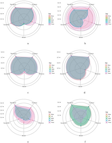
In general, we observed that the Vtreat imputation method consistently improves both the classification and regression performance compared to the other methods. Its superiority appears in almost all evaluation measures and cases. Interestingly, we observe a significant improvement for the Deep Neural Network and k-Nearest Neighbors concerning classification and regression. A minor difference is observed in logistic and linear regression for classification and regression performance, respectively. Additionally, we observe that the combination of XGBoost and Vtreat outperforms any other method/combination for both regression and classification tasks. Given that XGBoost is an efficient, cutting-edge classification technique, Vtreat reveals its true potential by enhancing its performance. Also, we observe that Vtreat significantly improves the performance of both DNN models known to perform better for unstructured data, such as images and text.

Visualizing the Prediction Power

Visualization is a central part of ML approaches since it offers insights into the data structure. Most visualization approaches apply a dimensionality reduction technique to transform the multidimensional data into two or three dimensions while preserving their relationships. Here, we focus on visualizing each imputation method’s predictive power through a two-dimensional representation. For this purpose, we employed the Principal Components Regression (PCR) technique to predict the HealthStatus score. Through this, we can investigate prediction power along with the corresponding two-dimensional representation produced by the respective Principal Component Analysis (PCA) method. Our motivation also lies in PCR’s advantages in both statistical and computational aspects, which reduce the variance estimation at the expense of other bias and offers a better model fitting (Slawski et al. 2018).

Briefly, let $A\in R^{s\times d}$ be the ATHLOS dataset, where $s$ is the number of samples, and $d$ is the number of predictor variables after applying the significant pruning step. Let $H\in R^{s\times 1}$ denote the vector of HealthStatus scores. Through PCR, we initially perform PCA on the centered data matrix $A$ and subsequently only consider the first two principal components, producing the matrix $A^{PC}\in R^{s\times 2}$. For the $N$ number of principal components, the formula for the HS evaluation is calculated as:

$HSEvaluation=a_0+\sum _{i=1}^p{a}_i{A}_i^{PC},$

where $a_0$ is the intercept, $a_i$ is the $i^{th}$ regression coefficient and $A_i^{PC}$ is the $i^{th}$ principal component resulted from PCA. The PCR technique is applied upon all five datasets produced by the application of each corresponding imputation method.

Initially, we observe that the low, medium and high values of the HealthStatus score exhibit better separability for the Vtreat method. In addition, observing the class distribution with respect to the first Principal Component, a clear distinction between classes is only achieved for the Vtreat method, while the respective distributions arising from LR, Mean, and DIM imputation methods have quite similar behavior (see Figure 2 for details).

Figure 2. Scatter plots (left column) depict the first two principal components of PCA performed on the five imputed ATHLOS datasets using Linear Regression, Mean, Dual Imputation Model, and Vtreat imputation. Circular points with orange, yellow, and light blue colors illustrate the low, medium, and high HS scores. Above and right to each scatter plot, their data distribution is illustrated. Heatmap-Scatter plots (right column) depict the correlation of predicted and real HS score of the five imputation methods using the Principal Components Regression (PCR) technique. The red to green color graduation of boxes indicates the number of samples from low to high amounts, respectively. Above and right to each heatmap-scatter plot is illustrated the marginal distribution of the HS and the HS estimation as univariate histograms with a density curve on the vertical and horizontal axes of the scatter plot, respectively

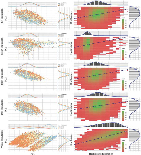
Utilizing the PCR technique to visualize regression efficiency (see Figure 2, right column) allows us to observe that the best performance is achieved by the Vtreat method, indicated by the higher correlation between predicted and real HS scores. Zooming into the respective heatmap-scatter, we can see the high number (green graduation in boxes) of samples across the dashed line, highlighting the optimal regression as reported in Table 2. We also observe all other methods perform poorly compared to Vtreat, while the mean imputation method behaves differently from the other two, with almost identical results.

Table 2. Comparison of 5 imputation methods using the Principal Components Regression technique. The table contains the (%) of the R-squared measure and the mean (standard error) values of Root Mean Square Error (RMSE). The best value among imputation methods for each measure is depicted in bold

	LR	Mean	MLR	DIM	Vtreat
R-squard	6.07	2.89	5.93	4.9	43.5
RMSE	9.705	9.862	9.733	9.767	7.545

Feature Importance for HealthStatus Prediction

Here, we aim to identify the factors that significantly affect HealthStatus prediction. Based on the indicated performance evaluation within the aforementioned experimental analysis, we captured this information by isolating the variable importance measure of the XGBoost algorithm when applied to the dataset imputed using the Vtreat methodology. The tree-based nature of this algorithm allowed us to export the relative importance or contribution of each input variable in predicting the response.

Let $T$ be a single decision tree, based on (Rights and Sterba 2020). We apply the following equation as an index of relevance for each of our features (predictor variables) $X_{\mathrm{\ell }}$:

${\mathcal{I}}_{\mathrm{\ell }}^2(T)=\sum _{t=1}^{J-1}{\hat{i}}_t^{2}I(v(t)=\mathrm{\ell }),$

where $J-1$ indicates the internal nodes of the tree, $t$ indicates each one of the input variables $X_{v(t)}$ and ${\hat{i}}_t^2$ indicates the maximal estimated improvement which defines the particular variable in squared error risk over that for a constant fit over the entire region ${\hat{i}}_t^2$. Utilizing this equation through the XGBoost model (Chen and Guestrin 2016), we obtain a list of the importance of each feature.

The results illustrated in Figure 3 offer new insights for the HealthStatus evaluation. More specifically, the most important variables (left plot in Figure 3) regarding their effectiveness in the HealthStatus prediction were the features: “Respondent’s self-rated/self-reported health” (srh), “Age at time of measure” (age), “History of arthritis, rheumatism, or osteoarthritis” (“h_joint_disorders”), “Current depressive status” (depression), “Engage in vigorous exercise during the last two weeks” (vig_pa), “Highest score, to the nearest kg, of all hand grip measurements, regardless” (grip), “Psychological measure of anxiety symptoms” (anxiety_symp), “Weekly frequency of less vigorous exercise” (f_mod_pa), “Participant has paid employment” (employed), and “Highest level of formal education achieved” (education).

Figure 3. The horizontal bars illustrate the most (left) and the least (right) important variables regarding their effectiveness in the HealthStatus prediction by applying the XGBoost classification algorithm. The x-axis imprints the variable importance score, while the y-axis includes the feature names defined by the ATHLOS project (see supplementary sheet S1)

On the other hand, the least important features (right plot in Figure 3) were the “Current smoker, any type of tobacco smoking” (current_smoking), “Ever experienced any natural disaster” (nat_dis), “Respondent is the participant, spouse/partner or other” (respondent), “Serum HDL Cholesterol” (hdl_chol), “Triglycerides” (triglycerides), “Experience of divorce/separation” (divorce), “Blood/serum glucose levels” (glucose), “Total Cholesterol” (total_chol), “Serum LDL Cholesterol” (ldl_chol) and “Is the relationship with the spouse close” (close_spouse).

Through the variable importance analysis, we interestingly observe that there are factors that significantly affect HealthStatus prediction while being unrelated to health, as well as factors that do not affect the HealthStatus but apparently should have, based on the recent literature. More specifically, the levels of depression were considered an important factor that affects the respondent’s HealthStatus prediction, a condition that exists at various age levels and does not necessarily indicate aging. Factors such as Serum HDL Cholesterol, Triglycerides, Blood/serum glucose levels, and Total Cholesterol were considered minor to determine the accurate HealthStatus prediction. However, all these factors are quite relevant to the human status health (Jian et al. 2017; Morgan and Mc Auley 2020).

Additionally, it is impressive how relevant is everyone’s personal opinion about assessing their state of health. Our results indicated that it is the most important factor. We may consider encouraging the fact that most can personally assess their state of health since this could affect prevention of adverse events and bad incidents, contributing to the Medical and Healthcare domain’s effectiveness that follows the participatory and preventive factors, two of the four main axes that constitute the future of Medicine (Hood 2017).

Meanwhile, the proposed framework can be adapted to various heterogeneous longitudinal medical (or health) studies, such as all COVID-19 related challenges. The more data we have, the better mining we can achieve for a case under study. A remarkable progress has been made regarding various COVID-19 issues (Chen et al. 2020; Lucas et al. 2020; Pierce et al. 2020; Wang et al. 2020b, 2020a).

Concluding remarks

In this paper, we emphasize developing a complete ML methodology for the ATHLOS (Aging Trajectories of Health: Longitudinal Opportunities and Synergies) Project, aiming in the accurate prediction of the HealthStatus (HS) score an index that estimates the human status of health. We deal with the most critical aspect of the inherent complexity of the provided dataset, the high degree of missing values by exploring extensively and discovering the most effective methodologies for missing value imputation. Our results indicated the effect of different imputation strategies on Machine Learning tasks exposing the capacity of accurate predictions when combined with cutting-edge tools. We additionally concluded that the highlighted Vtreat imputation method can be rendered as an imputation tool-guide for multiple unified, independent longitudinal studies. Finally, the variable importance analysis highlighted new factors that may affect the state of human health exposing the potential of further findings within similar large-scale longitudinal studies. In our future research, we intend to further investigate the development of a unified model on the basis of a bidirectional ML scheme for data imputation and prediction.

Acknowledgments

This work is supported by the ATHLOS (Ageing Trajectories of Health: Longitudinal Opportunities and Synergies) project, funded by the European Union’s Horizon 2020 Research and Innovation Programme under grant agreement number 635316.

Disclosure Statement

We confirm that the manuscript represents our own work, is original and has not been copyrighted, published, submitted, or accepted for publication elsewhere. We further confirm that we all have fully read the manuscript and give consent to be co-authors of the manuscript.

Supplementary Material

Supplemental data for this article can be accessed on the publisher’s website

Additional information

Funding

This research did not receive any specific grant from funding agencies in the public, commercial, or not-for-profit sectors.

References

- Andrews, G., F. Cheok, and S. Carr. 1989. The Australian longitudinal study of ageing. Australian Journal on Ageing 8 (2):31–35. doi:10.1111/j.1741-6612.1989.tb00756.x.
- Andrews, G., and M. J. Clark. 1999. The International Year of Older Persons: Putting aging and research onto the political agenda. The Journals of Gerontology Series B: Psychological Sciences and Social Sciences 54 (1): P7–P10. doi:10.1093/geronb/54B.1.P7.
- Arokiasamy, P., D. Bloom, J. Lee, K. Feeney, and M. Ozolins. 2012. Longitudinal aging study in India: Vision, design, implementation, and preliminary findings. National Research Council (US) Panel on Policy Research and Data Needs to Meet the Challenge of Aging in Asia; Smith JP, Majmundar M, editors. Aging in Asia: Findings From New and Emerging Data Initiatives. Washington (DC): National Academies Press (US)
- Azur, M. J., E. A. Stuart, C. Frangakis, and P. J. Leaf. 2011. Multiple imputation by chained equations: What is it and how does it work? International Journal of Methods in Psychiatric Research 20 (1):40–49. doi:10.1002/mpr.329.
- Börsch-Supan, A., M. Brandt, C. Hunkler, T. Kneip, J. Korbmacher, F. Malter, B. Schaan, S. Stuck, and S. Zuber. 2013. Data resource profile: the Survey of Health, Ageing and Retirement in Europe (SHARE). International journal of epidemiology 42 (4):992–1001. doi:10.1093/ije/dyt088
- Buuren, S. van, and K. Groothuis-Oudshoorn. 2010. mice: Multivariate imputation by chained equations in R. Journal of Statistical Software. In press:1–68.
- Caballero, F. F., G. Soulis, W. Engchuan, A. Sánchez-Niubó, H. Arndt, J. L. Ayuso-Mateos, J. M. Haro, S. Chatterji, and D. B. Panagiotakos. 2017. Advanced analytical methodologies for measuring healthy ageing and its determinants, using factor analysis and machine learning techniques: The ATHLOS project. Scientific Reports 7 (1):43955. doi:10.1038/srep43955.
- Cahan, E. M., T. Hernandez-Boussard, S. Thadaney-Israni, and D. L. Rubin. 2019. Putting the data before the algorithm in big data addressing personalized healthcare. NPJ Digital Medicine 2 (1):1–6. doi:10.1038/s41746-019-0157-2.
- Canela, M. Á., I. Alegre, and A. Ibarra. 2019. Dummy Variables. In: Quantitative Methods for Management, 57–63. Springer, Cham. doi: 10.1007/978-3-030-17554-2_6.
- Chai, T., and R. R. Draxler. 2014. Root mean square error (RMSE) or mean absolute error (MAE)?–Arguments against avoiding RMSE in the literature. Geoscientific Model Development 7 (3):1247–50. doi:10.5194/gmd-7-1247-2014.
- Chen, R., L. Sang, M. Jiang, Z. Yang, N. Jia, F. Wanyi, J. Xie W. Guan, W. Liang, Z. Ni, et al.. 2020. Longitudinal hematologic and immunologic variations associated with the progression of COVID-19 patients in China. Journal of Allergy and Clinical Immunology. 146(1):89–100. doi:10.1016/j.jaci.2020.05.003.
- Chen, T., and C. Guestrin. 2016. “Xgboost: A scalable tree boosting system.” In Proceedings of the 22nd ACM SIGKDD international conference on knowledge discovery and data mining, New York, NY, USA, 785–794.
- Dash, S., S. K. Shakyawar, M. Sharma, and S. Kaushik. 2019. Big data in healthcare: Management, analysis and future prospects. Journal of Big Data 6 (1):1–25. doi:10.1186/s40537-019-0217-0.
- DeSilva, A. P., M. Moreno-Betancur, A. M. De Livera, K. J. Lee, and J. A. Simpson. 2017. A comparison of multiple imputation methods for handling missing values in longitudinal data in the presence of a time-varying covariate with a non-linear association with time: A simulation study. BMC Medical Research Methodology 17 (1):1–11. doi:10.1186/s12874-017-0372-y.
- DeSilva, A. P., M. Moreno-Betancur, A. M. De Livera, K. J. Lee, and J. A. Simpson. 2019. Multiple imputation methods for handling missing values in a longitudinal categorical variable with restrictions on transitions over time: A simulation study. BMC Medical Research Methodology 19 (1):1–14. doi:10.1186/s12874-018-0650-3.
- Dimopoulos, A. C., M. Nikolaidou, F. F. Caballero, W. Engchuan, A. Sanchez-Niubo, H. Arndt, J. L. Ayuso-Mateos, J. M. Haro, S. Chatterji, E. N. Georgousopoulou, et al.. 2018. Machine learning methodologies versus cardiovascular risk scores, in predicting disease risk. BMC Medical Research Methodology. 18(1):1–11. doi:10.1186/s12874-018-0644-1.
- Eckle, K., and J. Schmidt-Hieber. 2019. A comparison of deep networks with ReLU activation function and linear spline-type methods. Neural Networks 110:232–42. doi:10.1016/j.neunet.2018.11.005.
- Eekhout, I., H. CW de Vet, J. W. R. Twisk, J. P. L. Brand, R. D. B. Michiel, and M. W. Heymans. 2014. Missing data in a multi-item instrument were best handled by multiple imputation at the item score level. Journal of Clinical Epidemiology 67 (3):335–42. doi:10.1016/j.jclinepi.2013.09.009.
- Elmessiry, A., W. O. Cooper, T. F. Catron, J. Karrass, Z. Zhang, and M. P. Singh. 2017. Triaging patient complaints: Monte Carlo cross-validation of six machine learning classifiers. JMIR Medical Informatics 5 (3):e19. doi:10.2196/medinform.7140.
- Flitcroft, L., W. S. Chen, and D. Meyer. 2020. The Demographic Representativeness and Health Outcomes of Digital Health Station Users: Longitudinal Study. Journal of Medical Internet Research 22 (6):e14977. doi:10.2196/14977.
- Hood, L. 2017. P4 medicine and scientific wellness: Catalyzing a revolution in 21st century medicine. Molecular Frontiers Journal 1 (2):132–37. doi:10.1142/S2529732517400156.
- Hosmer Jr, D. W., S. Lemeshow, and R. X. Sturdivant. 2013. Applied logistic regression. Vol. 398. John Wiley & Sons.
- Huque, M. H., J. B. Carlin, J. A. Simpson, and K. J. Lee. 2018. A comparison of multiple imputation methods for missing data in longitudinal studies. BMC Medical Research Methodology 18 (1):168. doi:10.1186/s12874-018-0615-6.
- Ichimura, H., S. Shimizutani, and H. Hashimoto. 2009. JSTAR first results 2009 report. Technical Report. Research Institute of Economy, Trade and Industry (RIETI).
- Jian, S., N. Su-Mei, C. Xue, Z. Jie, and W. Xue-sen. 2017. Association and interaction between triglyceride–glucose index and obesity on risk of hypertension in middle-aged and elderly adults. Clinical and Experimental Hypertension 39 (8):732–39. doi:10.1080/10641963.2017.1324477.
- Jolani, S., L. E. Frank, and S. van Buuren. 2014. Dual imputation model for incomplete longitudinal data. British Journal of Mathematical and Statistical Psychology 67 (2):197–212. doi:10.1111/bmsp.12021.
- Jordanov, I., N. Petrov, and A. Petrozziello. 2018. Classifiers accuracy improvement based on missing data imputation. Journal of Artificial Intelligence and Soft Computing Research 8 (1):31–48. doi:10.1515/jaiscr-2018-0002.
- Kelly, D., K. Curran, and B. Caulfield. 2017. Automatic prediction of health status using smartphone-derived behavior profiles. IEEE Journal of Biomedical and Health Informatics 21 (6):1750–60. doi:10.1109/JBHI.2017.2649602.
- Koskinen, S. 2018. “Health 2000 and 2011 Surveys—THL Biobank. National Institute for Health and Welfare.” https://thl.fi/fi/web/thl-biobank/for-researchers/sample-collections/health-2000-and-2011-surveys. [ Online; accessed 18-July-2008].
- Kowal, P., S. Chatterji, N. Naidoo, R. Biritwum, W. Fan, R. L. Ridaura, T. Maximova, P. Arokiasamy, N. Phaswana-Mafuya, S. Williams, et al.. 2012. Data resource profile: The World Health Organization Study on global AGEing and adult health (SAGE). International Journal of Epidemiology. 41(6):1639–49. doi:10.1093/ije/dys210.
- Kramer, O. 2013. K-nearest neighbors. In Dimensionality reduction with unsupervised nearest neighborsIntelligent Systems Reference Library, vol 51. Springer, Berlin, Heidelberg. https://doi.org/10.1007/978-3-642-38652-7_2.
- Leonardi, M., S. Chatterji, S. Koskinen, J. L. Ayuso-Mateos, J. M. Haro, G. Frisoni, L. Frattura, A. Martinuzzi, B. Tobiasz-Adamczyk, M. Gmurek et al.. 2014. Determinants of health and disability in ageing population: The COURAGE in Europe Project (collaborative research on ageing in Europe). Clinical Psychology & Psychotherapy. 21(3):193–98. doi:10.1002/cpp.1856.
- Licher, S., M. J. G. Leening, P. Yilmaz, F. J. Wolters, J. Heeringa, P. J. E. Bindels, Alzheimer’s Disease Neuroimaging Initiative, M. W. Vernooij, B. C. Stephan, E. W. Steyerberg et al.. 2019. Development and validation of a dementia risk prediction model in the general population: An analysis of three longitudinal studies. American Journal of Psychiatry 176(7):543–51. doi:10.1176/appi.ajp.2018.18050566.
- Lin, W.-C., and C.-F. Tsai. 2020. Missing value imputation: A review and analysis of the literature (2006–2017). Artificial Intelligence Review 53 (2):1487–509. doi:10.1007/s10462-019-09709-4.
- Liu, Y.-M. 2020. Population Aging, Technological Innovation, and the Growth of Health Expenditure: Evidence From Patients With Type 2 Diabetes in Taiwan. Value in Health Regional Issues 21:120–26. doi:10.1016/j.vhri.2019.07.012.
- Lucas, C., P. Wong, J. Klein, T. B. R. Castro, J. Silva, M. Sundaram, M. K. Ellingson, T. Mao, J. E. Oh, B. Israelow, et al.. 2020. Longitudinal analyses reveal immunological misfiring in severe COVID-19. Nature. 584(7821):463–69. doi:10.1038/s41586-020-2588-y.
- Luszcz, M. A., L. C. Giles, K. J. Anstey, C. B.-Y. Kathryn, R. A. Walker, and T. D. Windsor. 2016. Cohort Profile: The Australian Longitudinal Study of Ageing (ALSA). International Journal of Epidemiology 45 (4):1054–63. doi:10.1093/ije/dyu196.
- Marois, G., and A. Aktas. 2020. Projecting health trajectories in Europe using microsimulation. IIASA Working Paper. Laxenburg, Austria: WP-20-004.
- Miles, J. 2014. R squared, adjusted R squared. Wiley StatsRef: Statistics Reference Online. doi:10.1002/9781118445112.stat06627.
- Montgomery, D. C., E. A. Peck, and G. G. Vining. 2021. Introduction to linear regression analysis. John Wiley & Sons, Inc.
- Morgan, A. E. and M. T. Mc Auley 2020. Cholesterol Homeostasis: An In Silico Investigation into How Aging Disrupts Its Key Hepatic Regulatory Mechanisms. Biology 9 (10):314.
- Nooraee, N., G. Molenberghs, J. Ormel, R. Edwin, and V. D. Heuvel. 2018. Strategies for handling missing data in longitudinal studies with questionnaires. Journal of Statistical Computation and Simulation 88 (17):3415–36. doi:10.1080/00949655.2018.1520854.
- Panaretos, D., E. Koloverou, A. C. Dimopoulos, G.-M. Kouli, M. Vamvakari, G. Tzavelas, C. Pitsavos, and D. B. Panagiotakos. 2018. A comparison of statistical and machine-learning techniques in evaluating the association between dietary patterns and 10-year cardiometabolic risk (2002–2012): The ATTICA study. British Journal of Nutrition 120 (3):326–34. doi:10.1017/S0007114518001150.
- Park, J. H., S. Lim, J. Lim, K. Kim, M. Han, I. Y. Yoon, J. Kim, Y. Chang, C. B. Chang, H. J. Chin, et al.. 2007. An overview of the Korean longitudinal study on health and aging. Psychiatry Investigation 4 (2):84.
- Passarino, G., F. De Rango, and A. Montesanto. 2016. Human longevity: Genetics or Lifestyle? It takes two to tango. Immunity & Ageing 13 (1):12. doi:10.1186/s12979-016-0066-z.
- Peasey, A., M. Bobak, R. Kubinova, S. Malyutina, A. Pajak, A. Tamosiunas, H. Pikhart, A. Nicholson, and M. Marmot. 2006. Determinants of cardiovascular disease and other non-communicable diseases in Central and Eastern Europe: Rationale and design of the HAPIEE study. BMC Public Health 6 (1):255. doi:10.1186/1471-2458-6-255.
- Pedersen, A. B., E. M. Mikkelsen, D. Cronin-Fenton, N. R. Kristensen, T. M. Pham, L. Pedersen, and I. Petersen. 2017. Missing data and multiple imputation in clinical epidemiological research. Clinical Epidemiology 9:157. doi:10.2147/CLEP.S129785.
- Pierce, M., H. Hope, T. Ford, S. Hatch, M. Hotopf, A. John, E. Kontopantelis, R. Webb, S. Wessely, S. McManus, et al.. 2020. Mental health before and during the COVID-19 pandemic: A longitudinal probability sample survey of the UK population. The Lancet Psychiatry. 7(10):883–92. doi:10.1016/S2215-0366(20)30308-4.
- Prina, A. M., D. Acosta, I. Acosta, M. Guerra, Y. Huang, A. T. Jotheeswaran, I. Z. Jimenez-Velazquez, Z. Liu, J. J. Llibre Rodriguez, A. Salas, et al.. 2016. Cohort profile: The 10/66 study. International Journal of Epidemiology 46 (2):406–406i.
- Ribeiro, C., and A. A. Freitas. 2021. A data-driven missing value imputation approach for longitudinal datasets. Artificial Intelligence Review: 1–31. doi:10.1007/s10462-021-09963-5.
- Rights, J. D., and S. K. Sterba. 2020. New recommendations on the use of R-squared differences in multilevel model comparisons. Multivariate Behavioral Research 55 (4):568–99. doi:10.1080/00273171.2019.1660605.
- Rodríguez-Artalejo, F., A. Graciani, P. Guallar-Castillón, M. L. Luz, M. C. Zuluaga, E. López-García, J. L. Gutiérrez-Fisac, J. M. Taboada, M. T. Aguilera, E. Regidor, et al.. 2011. Rationale and methods of the study on nutrition and cardiovascular risk in Spain (ENRICA). Revista Española De Cardiología (English Edition). 64(10):876–82. doi:10.1016/j.rec.2011.05.023.
- Sanchez-Niubo, A., L. Egea-Cortés, B. Olaya, F. F. Caballero, L. A.-M. Jose, M. Prina, M. Bobak, H. Arndt, B. Tobiasz-Adamczyk, A. Pająk, et al.. 2019. Cohort profile: The Ageing trajectories of health–longitudinal opportunities and synergies (ATHLOS) project. International Journal of Epidemiology. 48(4):1052–1053i. doi:10.1093/ije/dyz077.
- Singh, S., and J. Prasad. 2013. Estimation of missing values in the data mining and comparison of imputation methods. Mathematical Journal of Interdisciplinary Sciences 1 (2):75–90. doi:10.15415/mjis.2013.12015.
- Slawski, M.. 2018. On principal components regression, random projections, and column subsampling. Electronic Journal of Statistics. 12(2):3673–712. doi:10.1214/18-EJS1486.
- Sonnega, A., J. D. Faul, M. B. Ofstedal, K. M. Langa, J. W. R. Phillips, and D. R. Weir. 2014. Cohort profile: The health and retirement study (HRS). International Journal of Epidemiology 43 (2):576–85. doi:10.1093/ije/dyu067.
- Stavseth, M. R., T. Clausen, andJ. Røislien. 2019. How handling missing data may impact conclusions: A comparison of six different imputation methods for categorical questionnaire data. SAGE Open Medicine 7:2050312118822912. doi:10.1177/2050312118822912.
- Steptoe, A., E. Breeze, J. Banks, and J. Nazroo. 2013. Cohort profile: The English longitudinal study of ageing. International Journal of Epidemiology 42 (6):1640–48. doi:10.1093/ije/dys168.
- Tai, A. M. Y., A. Albuquerque, N. E. Carmona, M. Subramanieapillai, D. S. Cha, M. Sheko, Y. Lee, R. Mansur, and R. S. McIntyre. 2019. Machine learning and big data: Implications for disease modeling and therapeutic discovery in psychiatry. Artificial intelligence in medicine 99:101704. doi:10.1016/j.artmed.2019.101704.
- Vilardell, M., M. Buxó, R. Clèries, J. M. Martínez, G. Garcia, A. Ameijide, R. Font, S. Civit, R. Marcos-Gragera, M. L. Vilardell, and M. Carulla. 2020. Missing data imputation and synthetic data simulation through Modeling Graphical Probabilistic Dependencies between Variables (ModGraProDep): An application to breast cancer survival. Artificial Intelligence in Medicine 107:101875. doi:10.1016/j.artmed.2020.101875.
- Wang, C., R. Pan, X. Wan, Y. Tan, X. Linkang, S. M. Roger, F. N. Choo, B. Tran, R. Ho, V. K. Sharma, et al.. 2020a. A longitudinal study on the mental health of general population during the COVID-19 epidemic in China. Brain, Behavior, and Immunity 87:40–48. doi:10.1016/j.bbi.2020.04.028.
- Wang, Y., C. Dong, H. Yue, L. Chungao, Q. Ren, X. Zhang, H. Shi, and M. Zhou. 2020b. Temporal changes of CT findings in 90 patients with COVID-19 pneumonia: A longitudinal study. Radiology 296 (2):E55–E64. doi:10.1148/radiol.2020200843.
- Whelan, B. J., and G. M. Savva. 2013. Design and methodology of the Irish Longitudinal Study on Ageing. Journal of the American Geriatrics Society 61:S265–S268. doi:10.1111/jgs.12199.
- Wiens, J., and E. S. Shenoy. 2018. Machine learning for healthcare: On the verge of a major shift in healthcare epidemiology. Clinical Infectious Diseases 66 (1):149–53. doi:10.1093/cid/cix731.
- Wong, R., A. Michaels-Obregon, and A. Palloni. 2017. Cohort profile: The Mexican health and aging study (MHAS). International Journal of Epidemiology 46 (2):e2–e2. doi:10.1093/ije/dyu263.
- Yamaguchi, Y., M. Ueno, K. Maruo, and M. Gosho. 2020. Multiple imputation for longitudinal data in the presence of heteroscedasticity between treatment groups. Journal of Biopharmaceutical Statistics 30 (1):178–96. doi:10.1080/10543406.2019.1632878.
- Zhang, Y., G. Golm, and G. Liu. 2020. A likelihood-based approach for the analysis of longitudinal clinical trials with return-to-baseline imputation. Statistics in Biosciences 12 (1):23–36. doi:10.1007/s12561-020-09269-0.
- Zhang, Z. 2016. Introduction to machine learning: K-nearest neighbors. Annals of Translational Medicine 4:11. doi:10.21037/atm.2016.03.37.
- Zhao, J., Q. Feng, P. Wu, R. A. Lupu, R. A. Wilke, Q. S. Wells, J. C. Denny, and W.-Q. Wei. 2019. Learning from longitudinal data in electronic health record and genetic data to improve cardiovascular event prediction. Scientific Reports 9 (1):1–10. doi:10.1038/s41598-018-37186-2.
- Zhou, L., S. Pan, J. Wang, and A. V. Vasilakos. 2017. Machine learning on big data: Opportunities and challenges. Neurocomputing 237:350–61. doi:10.1016/j.neucom.2017.01.026.
- Zumel, N., and J. Mount. 2016. vtreat: A data. frame Processor for Predictive Modeling. In arXiv preprintarXiv:1611.09477v9.
- Zumel, N., J. Mount, and J. Porzak. 2014. Practical data science with R. New York, NY, USA, Manning Shelter Island.