Predicting stock price movement using a DBN-RNN

ABSTRACT

This paper proposes a deep learning-based model to predict stock price movements. The proposed model is composed of a deep belief network (DBN) to learn the latent feature representation from stock prices, and a long short-term memory (LSTM) network to exploit long-range relations within the trading history. The prediction target of the model is the stock close price direction on the next day. To predict the trend of one stock, the feature of recent trading information is generated from the raw intra-day data through a pre-trained DBN. Then the extracted features are fed into an LSTM classifier to produce the prediction result for the next day. The proposed model was tested on 36 companies in the Shanghai Stock Exchange (SSE) and the Shenzhen Stock Exchange (SZSE), which were selected based on their weights in Chinese A-shares. The experiments cover a span of 12 years, from 2005 to 2016, and the results show that the proposed model offers notable improvements in predicting performance comparing with other learning models. It is also observed that some companies are more predictable than others, which implies that the proposed model can be used for financial portfolio construction.

Introduction

Prediction of the stock market is a popular research topic in both financial marketing and data fields. Investors, as well as researchers, hope to gain profit from investments by predicting the trend of the overall market or individual stocks. However, it is a challenging task to outperform skilled and knowledgeable competitors in stock markets. Better stock price direction prediction is a key factor for successful decision-making and for building trading strategy. Also, it gives early warning to investors about sudden drops in the market, especially for short-term investments.

As Giles et al. (Lee Giles, Lawrence, and Tsoi 2001) explained, challenges faced in stock predicting include small sample size, high noise, non-stationarity, and non-linearity of the market, which is related to a number of factors, including political events, market news, quarterly earning reports, conflicting trading behavior, etc. Traders often rely on technical indicators based on stock data that can be collected on a daily basis. Despite the availability of these indicators, it is often difficult to achieve satisfactory prediction accuracy in the actual stock market. In fact, the high level of noise in the financial market makes it hard even for professional investors to predict price movements using public information. Financial experts still argue about whether financial time series are predictable, while researchers are already proposing various prediction models and developing different trading strategies based on those models. Prior studies demonstrated that artificial intelligence (AI) approaches, especially neural-network approaches, are helpful in stock prediction. For example, Saad, Prokhorov, and Wunsch (1998) compared three neural networks to predict stock trends while the focus was on limiting the false alarm rate. The networks used in the experiments were time delay, recurrent, and probabilistic neural networks. They declared feasible results on all the networks. Likewise, a number of researchers have utilized feed-forward neural networks and recurrent neural networks for forecasting and modeling financial markets (Lee 2006; Lin, Yang, and Song 2009; Mostajabi, Yadollahpour, and Shakhnarovich 2015; Pui Cheong Fung, Yu, and Lam 2003; Schumaker and Chen 2009; Tsai and Hsiao 2010).

A practical issue arises when applying neural networks in stock prediction. The stock market is highly complicated and multifaceted and is easily affected by economical and political factors. Some researchers take technical indices and qualitative factors into account in stock market precollected through python interfaceediction (Schumaker and Chen 2009; Tsai and Hsiao 2010). Other researchers use news articles to extract information and knowledge to help them analyze the stock market (Hao 2010; Kim and Chun 1998). However, it is often difficult for investors to collect these auxiliary data for further analysis. On the other hand, historical stock prices of multiple granularities are easily acquired through open interfaces on the internet. We believe that long-term stock price movements can reflect outlier factors to a large extent, making it possible to predict stock price based only on historical prices. In this paper, we show that this method gives excellent results in prediction accuracy and is feasible to make money in the actual stock market.

Another issue in predicting stock price using neural networks is the choice of sample size, which is determined by real-world transaction records over a certain period. On one hand, a smaller sample size refers to a shorter period of transaction records and could be insufficient for training a prediction model; on the other hand, a large sample size increases the uncertainty of the financial environment during the sample period. For instance, the development of a country’s stock market is closely related to the country’s economic development. When a country’s economic situation changes significantly, its stock market will be subject to violent fluctuations, which makes past experience inadequate to help predict the future of the stock market.

This paper seeks to find answers to the questions above. An automatic stock predicting model is proposed based on the deep-learning technique, namely deep belief network (DBN), and long short-term memory (LSTM). The prediction model is built upon intra-day stock data, where the purpose of using intra-day data instead of daily data is to enrich the sample information within a short period of time. In experiments carried out in Section 5, the model is trained on a 2-year training set, which eliminates the training data variance due to financial environment changes. The proposed model is composed of two deep-learning techniques: DBN is applied to extract daily features from raw stock intra-day data, and a LSTM neural network is then applied to predict the stock movements based on extracted features. At first, the DBN parameters are pre-trained via unsupervised learning using the raw input data. Next, both the DBN and LSTM are fine-tuned in a supervised manner, with labeled samples, using a back-propagation algorithm. The final output of the LSTM classifier is a binary vector that indicates the probability of the stock’s trend the next day.

This paper also seeks to answer whether the trading strategy based on a technical analysis is valid or not. Although many previous works showed successful results, most of them conducted tests within the in-sample datasets, which indicates that the trained model may fail to generalize to real markets, or the out-of-sample testing was performed on a small number of stocks during a short period, which is unlikely to represent the full market behavior. In order to overcome those drawbacks, in this paper, the tests were performed using sliding windows to ensure that the predictions were made on most available test years, and only the recent year information was used to make predictions, while old data that were probably no longer relevant in the context of a dynamic, rapidly evolving stock market were not incorporated. For example, when testing on year Y, year Y-3 and Y-2 were used for training the prediction model, while year Y-1 was used as a validation set to adjust parameters. In this paper, experiments were performed with 36 major stocks from the Chinese stock market for 12 years to validate the performance of the model. A wide range of tests are important since the goal of the stock prediction system is to choose predictable stocks among a number of companies.

The remainder of this paper is organized as follows: Section 2 presents related works carried out in the stock price predicting field. Section 3 describes the proposed approach in detail. Section 4 describes the setup of experiments and discusses some useful techniques in training. Section 5 shows the test results on real stock data. A conclusion and future work discussions are presented in Section 6.

The Proposed Stock Prediction Model

The architecture of the proposed model is a hybrid deep learning framework consisting of two major stages: a feature-extraction stage and a classification stage. A component wise description follows:

Data Description and Objective

The study covers the time period of January 4, 2005 through October 25, 2016. We used data of 36 stocks in the Shanghai Stock Exchange (SSE) and Shenzhen Stock Exchange (SZSE), two major stock exchanges in China. The tested stocks were selected from the CSI 300 index.¹ We chose stocks with the highest relative weight in the market, and excluded stocks that came into the market after 2005 or had been suspended for more than a year between 2005 and 2016 in order to maintain the consistency of the test. The test data was collected through python interfaces provided by the Tushare toolkit (Github 2016). The historical statistics were high-frequency trading data including the trading price, trading time and trading volume information. The minute data and daily data can be generated using those high-frequency trading data.

In this study, the objective is to predict the stock price direction on the next day, hence the prediction result is defined as a binary value: 0 for up and 1 for down. The problem can be described as a kind of time-series data prediction with the form:

(1) $target(t+1)=f(g(x(t)),g(x(t-1)),\dots )$(1)

Here, $target(t+1)$ represents the prediction result on day $t+1$, $x(t)$ is raw intra-day data on day $t$, and $g(x)$ is a function to extract features from the input.

Deep Belief Network for Feature Generation

Data feature selection is one of the most important factors that affect the accuracy of a prediction model. In this study, a DBN consisting of stacked RBMs was used as the feature extractor where the raw stock data was used as the input.

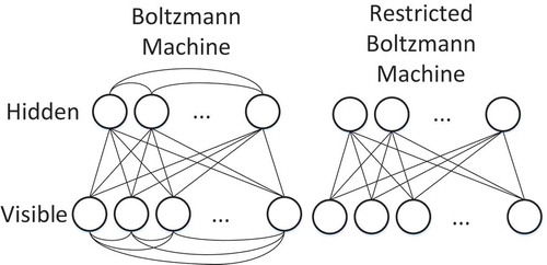
A DBN is a multi-layered probabilistic graphical model that learns to extract a deep hierarchy representation of the training data (Hinton et al. 2012). It consists of simpler undirected graphical models, i.e. restricted Boltzmann machines (RBMs), typically with stochastic binary units. An RBM has a bottom layer of ’visible’ units, and a top layer of ’hidden’ units, which are fully and bidirectionally connected with symmetric weights. The difference between standard Boltzmann machines and RBMs is that in the restricted model units within the same layer are not connected (see Figure 1), which makes inference and learning within this graphical model tractable. A Boltzmann machine can be expressed as an energy model where the energy is a linear function of the free parameters as follows:

(2) $E(v,h)=-{b^{\prime }}_{v}v-{b^{\prime }}_{h}h-h^{\prime }Wv$(2)

Figure 1. Boltzmann and restricted Boltzmann machines

In Eq. 2(2) $E(v,h)=-{b^{\prime }}_{v}v-{b^{\prime }}_{h}h-h^{\prime }Wv$(2) W represents the weights between the hidden layer units (h) and the visible layer units (v). $b_v$ and $b_h$ are the biases of the visible and hidden layers, respectively.

Samples can be obtained from an RBM by performing block Gibbs sampling, where visible units are sampled simultaneously given fixed values of the hidden units. Similarly, hidden units are sampled simultaneously given the visible unit values. A single step in the Markov chain is thus taken as follows:

(3) $h^{n+1}=\delta (W^{\prime }{v}^{(n)}+b_h)$(3)

(4) $v^{n+1}=\delta (W{h}^{(n+1)}+b_v)$(4)

where $\delta$ represents the sigmoid function acting on the activations of the $(n+1{)}_{th}$ hidden and visible units. Several algorithms have been devised for RBMs in order to efficiently sample from $p(v,h)$ during the learning process, the most effective being the well-known contrastive divergence (CD-k) algorithm (Hinton 2002).

RBMs can be stacked and trained greedily to form deep belief networks (DBNs). The visible layers of RBMs at the bottom of a DBN are clamped to the actual inputs when data is presented. When RBMs are stacked to form a DBN, the hidden layer of the lower RBM becomes the visible layer of the next higher RBM. Through this process, higher level RBMs can be trained to encode more and more abstract features of the input distribution. A DBN models the joint distribution between the observed vector v and the hidden layers $h_k$ as follows:

(5) $P(v,h^1,\dots ,h^l)=(\prod _{k=0}^{l-2}P(h^k|h^{k+1}))P(h^{l-1},h^l)$(5)

where $v=h^0$, $P(h^{k-1}|h^k)$ is a conditional distribution for the visible units conditioned on the hidden units of the RBM at level k, and $P(h^{l-1}|h^l)$ is the visible-hidden joint distribution in the top-level RBM.

In this paper, five-minute bars of one day are treated as the basic units of the input to the DBN for further processing. The output of the DBN will be the extracted features of this day. In China exchanges the continuous auction runs from 9:30 to 11:30 and from 13:00 to 15:00, which indicates there exist 48 five-minute bars each day. In this paper, the input shape of DBN is set to $48\ast 5=240$ according to the number of indicators within each bar.

A two-layer DBN is used in the tests, where the DBN is first trained layer-by-layer in a pre-training step. Inspired by the Hinton (Hinton 2010) method, we split the dataset into smaller, non-overlapping mini-batches. The RBMs in the encoder are unrolled to form an encoder-decoder, which is fine-tuned using a back-propagation (BP) algorithm after the pre-training. In the implementation, the number of hidden units in the final layer of the encoder is sharply reduced, which forces reduction in dimensionality. At this stage, the encoder outputs a low dimensional representation of the inputs. The intention is that it retains interesting features from historical stock charts that are useful for forecasting returns, but eliminates irrelevant noise. After the training of the DBN in the first step is finished, the DBN can be used to extract features from raw stock data. The latent representation of the features is then used for constructing a classifier for the prediction goal defined above.

Long Short-Term Memory Recurrent Neural Network for Classification

A recurrent neural network (RNN) is similar to a multi-layer perception except for the recurrent vector to restore history information. An RNN is different from a standard neural network in that it takes a sequence $v=(v_1,v_2,\dots ,v_T)$ as input, and iterates over it from $t=1$ to T, to produce the following:

(6) $q_t=\delta (b_{qt}+W_{vq}{v}_t+W_{qq}{q}_{t-1})$(6)

where $q=(q_1,q_2,\dots ,q_T)$ is a vector representing the hidden unit. The b terms are bias vectors (e.g. $b_q$ represents bias of the hidden layer). The nonlinear function $\delta$ may vary with context and is usually the application of element-wise sigmoid ($\delta$) or tanh.

Long short-term memory (LSTM) (Hochreiter and Schmidhuber 1997) is one of the most successful RNN architectures. LSTM introduces the memory cell, a unit of computation that replaces traditional artificial neurons in the hidden layer of a network. With these memory cells, networks are able to effectively associate memories and inputs over long periods of time, hence they are suitable for grasping the structure of the data dynamically over time with high prediction capacity.

The structure of this neural network is shown in Figure 2. It has a dynamic gating mechanism. Running through the center is the cell state $I_i$ which is interpreted as the information flow of the market sensitivity. $I_i$ has a memory of past time information and more importantly, it learns to forget (Gers et al., 2000):

(7) $I_i=f_i\ast I_{i-1}+c_i\ast {\tilde{I}}_i$(7)

Figure 2. Representative LSTM

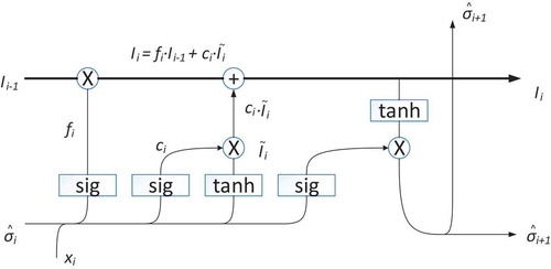
Here $f_i$ is the fraction of past-time information passed over to the present, ${\tilde{I}}_i$ measures the information flowing in at the current time and $c_i$ is the weight of how important this current information is. All three quantities are functions of the input $x_{\lambda ,i}$ and last-epoch’s estimation of volatility ${\tilde{\delta }}_i$.

(8) $f_i=sigmoid\left[\left({\hat{\delta }}_i,x_i\right)\ast W_f+b_f\right]$(8)

(9) $c_i=sigmoid\left[\left({\hat{\delta }}_i,x_i\right)\ast W_c+b_c\right]$(9)

(10) ${\tilde{I}}_i=tanh\left[\left({\hat{\delta }}_i,x_i\right)\ast W_{\tilde{I}}+b_{\tilde{I}}\right]$(10)

To make a prediction of the next volatility value ${\hat{\delta }}_{i+1}$, a linear activation function is used.

(11) ${\hat{\delta }}_{i+1}=\alpha +\beta \ast o_i\ast tanh\left[I_i\right]$(11)

Here $o_i$, which is also a function of $x_{\lambda ,i}$ and ${\hat{\delta }}_i$ tunes the output.

(12) $o_i=sigmoid\left[\left({\hat{\delta }}_i,x_i\right)\ast W_o+b_o\right]$(12)

$I_i$ and ${\hat{\delta }}_i$ are passed down to the next time step for continual predictions. Eq. 12(12) $o_i=sigmoid\left[\left({\hat{\delta }}_i,x_i\right)\ast W_o+b_o\right]$(12) answers the fundamental question of memory in time series forecasting.

In this study, the extracted features of the DBN are feed into an LSTM classifier for further processing. The LSTM classifier receives identical input which is the DBN output in the pre-training stage, and outputs the prediction result. The next step is to fine-tune the classifier network using the labeled examples via back-propagation. The classifier gives a binary output, which means the prediction result is either up or down, indicating the trend of the close price in the following day. Conventional training of a classifier consists of minimizing a cost function, in this study we chose the mean square error (MSE) at the LSTM output layer.

The DBN-LSTM Architecture

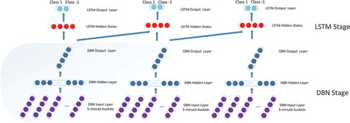
The DBN-LSTM is an extension of the generative model (RNN-DBN) proposed by (Goel, Vohra, and Sahoo 2014). There are a few significant im-provements made to this model, most notably the replacement of the RNN with an LSTM, which is a more powerful neural architecture capable of modeling temporal dependencies across large time steps. This ensures the model retains information about the sequence generated for a longer time duration. Particularly for generative models, this property lends itself exceptionally well to modeling creativity. In stock prediction, choosing LSTM over RNN results in better generalization, since the improved memory of the LSTM possess more information about previously trading information in the sequence as compared to an RNN. The complete pipeline of the architecture is illustrated in Figure 3.

Figure 3. Structure of the DBN-LSTM model

Experiment Setup

As discussed in Section 3, the proposed model is combined with a DBN receiving minute bars as input, and an LSTM to output prediction results in binary form.

Data Preprocessing

As mentioned above, the stock data used in this paper is 5-min OHLC (Open price/High price/Low price/Close price) bars, which indicates 48×5 = 240 data points each day. As to be expected, for such a large collection of data, there are missing values existing in the raw data. For a missing bar, a ’dummy’ bar is created where the trading volume is set to 0 and all four prices are set as the close price of the former bar.

In general, the stock price data have bias due to differences in time spans (Kamijo and Tanigawa 1990). Eliminating this bias requires normalization of the input data. It is also observed in previous research that applying normalization in the input layer of a neural network can decrease the influence of noise in the training data set, thus improving the generalization ability of the trained model (Ioffe and Szegedy 2015). In this paper, the data is divided into two groups which are OHLC prices and the trading volume, and each axis is normalized within the range [0,1] using a min-max normalization algorithm (Jain, Nandakumar, and Ross 2005).

Implementation Details

The deep learning library Theano (Al-Rfou et al. 2016) was used to implement the overall network architecture. The network was trained on a GPU server containing 8 NVIDIA Tesla K40c GPU cards with 12 GB memory each. We used a DBN-LSTM with two hidden DBN layers – each having 100 binary units – and 150 binary units in the LSTM. The visible layer of DBN had 50 binary units. The LSTM had a sequence length of 20. Dropout was incorporated in each layer. Only raw minute bar data was given as input to the DBN-LSTM. We evaluated our models qualitatively by generating sample sequences and quantitatively by using the mean square error (MSE) as a performance measure. The learning rate when pre-training the DBN was set at 0.1 and the max training epoch was 100. When fine-tuning the full DBN-LSTM network, the initial training rate was set at 0.01, and the learning rate decayed by half when the error at the LSTM output layer in this epoch was larger than that in last epoch. The training halted when the learning rate was smaller than ${10}^{-6}$.

Results and Analysis

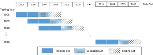
The stock data from January 2005 to October 2016 was divided into nine overlapping training-validation-testing sets, as shown in Figure 4. The test used the walk-forward routine, which is commonly used in evaluating the predictive performance of time-series data. To test on year Y, the model was trained on two consecutive years from year $Y-3$ to $Y-2$, and validated on year $Y-1$. The testing year shifted from 2008 to 2016.

Figure 4. Testing scheme used in this paper

Accuracy and Precision Evaluation

First, we analyzed the frequency of correct prediction of the proposed model on the test dataset. The results are shown in Figure 5, Figure 6 and Figure 7. We tested the model on predicting the close price trend on the following day. To predict the referred stock price trends, the goal is to predict

(13) $1\{P_{close}^{(t+1)}{P}_{close}^{(t)}\}$(13)

Figure 5. Accuracies and precisions of 36 test companies

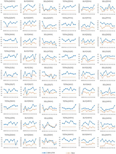
Figure 6. (Continued.) Accuracies and precisions of 36 test companies

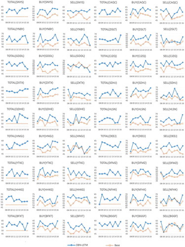
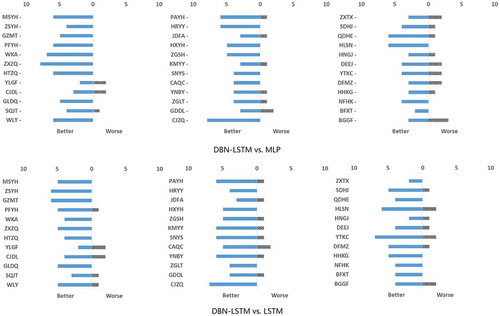
Figure 7. Comparison of DBN-LSTM with other approaches by companies

where $P_{close}^{(t)}$ is the close price today and $P_{close}^{(t+1)}$ represents the close price tomorrow.

To judge the performance of the prediction model, two standard evaluating metrics were used, namely accuracy and precision. There are two precision metrics evaluated in this paper, namely positive precision and negative precision. Specifically,

(14) $accuracy=\frac{\mathrm{\#}correctpredictions}{\mathrm{\#}totalpredictions}$(14)

(15) $positiveprecision=\frac{\mathrm{\#}correctuptickpredictions}{\mathrm{\#}totaluptickpredictions}$(15)

(16) $negativeprecision=\frac{\mathrm{\#}correctdowntickpredictions}{\mathrm{\#}totaldowntickpredictions}$(16)

In Figure 6 and Figure 7, there are three charts for each company, ’BUY’, ’SELL’ and ’TOTAL’. Here ’BUY’ and ’SELL’ charts refer to the positive and negative precision, respectively, and ’TOTAL’ is the accuracy regarding both positive and negative predictions. In ’BUY’ and ’SELL’ charts, ’base’ lines mean the percentage of days when the price rose and fell over the total number of days. Table 1 shows the average accuracy improvements over the base accuracy for each company. It is an interesting phenomenon that it has a larger improvement in ’BUY’ than in ’SELL’ in most cases.

Table 1. Average Accuracy Improvement over ’Base’ (%)

Symbols	TOTAL	BUY	SELL	Symbols	TOTAL	BUY	SELL
MSYH	8.70	18.89	−1.51	ZXTX	9.75	9.00	10.70
ZSYH	8.92	8.94	9.20	SDHJ	7.53	8.74	6.65
GZMT	9.53	15.36	4.18	QDHE	8.18	7.65	8.65
PFYH	9.77	10.39	9.72	HLSN	8.77	13.76	3.76
WKA	8.28	9.79	7.56	HNGJ	5.50	4.62	6.18
ZXZQ	8.42	11.29	6.22	DEEJ	8.43	11.12	6.00
HTZQ	9.72	15.38	4.55	YTKC	8.55	13.70	4.11
YLGF	6.18	10.06	2.31	DFMZ	8.97	15.91	1.17
CJDL	7.78	9.21	6.76	HHKG	9.64	17.16	1.88
GLDQ	10.69	17.38	4.25	NFHK	8.16	7.72	8.34
SQJT	7.61	7.76	7.86	BFXT	8.73	5.88	13.15
WLY	9.64	10.05	9.82	BGGF	6.15	7.53	4.97
PAYM	7.14	12.22	2.26	HRYY	8.47	12.12	4.69
JDFA	8.45	22.23	-5.86	HXYH	10.52	13.08	8.17
ZGSH	7.12	11.29	3.10	KMYY	9.60	7.56	11.33
SNYS	9.88	18.66	1.32	CAQC	8.09	7.04	9.39
YNBY	9.59	7.70	11.79	ZGLT	9.54	9.00	10.56
GDDL	8.58	9.90	6.12	CJZQ	10.06	13.66	6.64

Comparison with Other Models

We compared our model with two other models: one is multi-layer perception (MLP) with a sliding window size of five and two hidden layers of ten nodes, and another is LSTM without DBN. Unlike the proposed model where intra-day data is used for training, these two models do not have a feature-generation stage, and are built upon only daily data. Fig. 8 show the comparison results between the proposed approach and other ones by companies and years. In the figures, ‘better’ and ‘worse’ mean the number of cases where the final property of the DBN-LSTM is higher or lower that of the corresponding approach by 5% or more, respectively. The DBN-LSTM shows consistently better performance; it predicts better for 34 of the 36 companies than MLP. Also it predicts better for 35 of the 36 companies compared to LSTM.

Conclusion and Future Work

This paper describes a novel deep neural network architecture for stock movement prediction, which consists of a deep belief network and a long short-term memory recurrent neural network. The key idea behind the architecture is to offer a pre-training step to extract latent features based on raw stock data, which lets the classifier enjoy rich information when deciding whether the stock price will rise or fall. Test results on 36 Chinese heavyweight stocks show the efficiency and improved performance for such deep neural network architecture, which outperforms existing similar architectures. To the best of our knowledge, the combination of the DBN feature extractor with LSTM classifier using intra-day data is new for stock price forecasting. Due to its promising performance, we will apply the system for real-time daily trading.

The proposed model is conceptually suitable for using heterogeneous stock price data with further detailed information. In the future, additional data such as technical indicators and news articles can be integrated into this system to further explore the complex time-series problem. In addition, an intelligent trading system can be built that can automatically select candidate stocks from the market and construct a portfolio for real-time trading.

Notes

1. The CSI 300 list is available at http://www.csindex.com.cn/sseportal/csiportal/zs/jbxx/report.do?code=000300&subdir=1

References

- Team T T D, Al-Rfou R, Alain G, et al. Theano: A Python framework for fast computation of mathematical expressions[J]. arXiv preprint arXiv:1605.02688, 2016.
- Gers, F. A., J. Schmidhuber, and F. Cummins. 2000. Learning to forget: Continual prediction with lstm. Neural Computation 12 (10):2451–71. doi:https://doi.org/10.1162/089976600300015015.
- Github. Tushare: Utility for crawling historical data of china stocks. https://github.com/waditu/tushare, 2016.
- Goel, K., R. Vohra, and J. K. Sahoo. Polyphonic music generation by modeling temporal dependencies using a rnn-dbn[C]//International Conference on Artificial Neural Networks. Springer, Cham, Hanburg, Germany, 217-224, 2014.
- Hao, H.-N. Notice of retraction short-term forecasting of stock price based on genetic-neural network. In 2010 Sixth International Conference on Natural Computation, 4, 1838–41. IEEE, Yantai, China, 2010.
- Hinton, G. 2010. A practical guide to training restricted Boltzmann machines. Momentum 90 (1):926.
- Hinton, G., L. Deng, D. Yu, G. E. Dahl, A.-R. Mohamed, N. Jaitly, A. Senior, V. Vanhoucke, P. Nguyen, T. N. Sainath et al. 2012. Deep neural networks for acoustic modeling in speech recognition: The shared views of four research groups. IEEE Signal Processing Magazine. 29(6):082–97. doi:https://doi.org/10.1109/MSP.2012.2205597.
- Hinton, G. E. 2002. Training products of experts by minimizing contrastive divergence. Neural Computation 140 (8):1771–800. doi:https://doi.org/10.1162/089976602760128018.
- Hochreiter, S., and J. Schmidhuber. 1997. Long short-term memory. Neural Computation 9 (8):1735–80. doi:https://doi.org/10.1162/neco.1997.9.8.1735.
- Ioffe, S., and C. Szegedy. Batch normalization: Accelerating deep network training by reducing internal covariate shift. arXiv preprint arXiv:1502.03167, 2015.
- Jain, A., K. Nandakumar, and A. Ross. 2005. Score normalization in multimodal biometric systems. Pattern Recognition 38 (12):2270–85. doi:https://doi.org/10.1016/j.patcog.2005.01.012.
- Kamijo, K.-I., and T. Tanigawa. Stock price pattern recognition-a recurrent neural network approach[C]//1990 IJCNN international joint conference on neural networks. IEEE, San Diego, CA, USA, 215-221, 1990.
- Kim, S. H., and S. H. Chun. 1998. Graded forecasting using an array of bipolar predictions: Application of probabilistic neural networks to a stock market index. International Journal of Forecasting 14 (3):323–37. doi:https://doi.org/10.1016/S0169-2070(98)00003-X.
- Lee Giles, C., S. Lawrence, and A. C. Tsoi. 2001. Noisy time series prediction using recurrent neural networks and grammatical inference. Machine Learning 44 (1/2):161–83. doi:https://doi.org/10.1023/A:1010884214864.
- Lee, R. S. T. ijade stock advisor: An intelligent agent-based stock prediction system using the hybrid rbf recurrent network. Fuzzy-Neuro Approach to Agent Applications: From the AI Perspective to Modern Ontology, 231–53, 2006.
- Lin, X., Z. Yang, and Y. Song. 2009. Short-term stock price prediction based on echo state networks. Expert Systems with Applications 36 (3):7313–17. doi:https://doi.org/10.1016/j.eswa.2008.09.049.
- Mostajabi M., Yadollahpour P., and Shakhnarovich G. Feedforward semantic segmentation with zoom-out features[C]//Proceedings of the IEEE conference on computer vision and pattern recognition. Boston, MA, USA, 3376-3385, 2015.
- Fung G.P.C., Yu J.X., and Lam W. Stock prediction: Integrating text mining approach using real-time news[C]//2003 IEEE International Conference on Computational Intelligence for Financial Engineering, 2003. Proceedings. IEEE, Hong Kong, China, 395-402, 2003.
- Saad, E. W., D. V. Prokhorov, and D. C. Wunsch. 1998. Comparative study of stock trend prediction using time delay, recurrent and probabilistic neural networks. IEEE Transactions on Neural Networks 9 (6):1456–70. doi:https://doi.org/10.1109/72.728395.
- Schumaker, R. P., and H. Chen. 2009. A quantitative stock prediction system based on financial news. Information Processing & Management 45 (5):571–83. doi:https://doi.org/10.1016/j.ipm.2009.05.001.
- Tsai, C.-F., and Y.-C. Hsiao. 2010. Combining multiple feature selection methods for stock prediction: Union, intersection, and multi-intersection approaches. Decision Support Systems 50 (1):258–69. doi:https://doi.org/10.1016/j.dss.2010.08.028.