Swarm Intelligence-Based Feature Selection for Amphetamine-Type Stimulants (ATS) Drug 3D Molecular Structure Classification

ABSTRACT

Swarm intelligence-based feature selection techniques are implemented by this work to increase classifier performance in classifying Amphetamine-type Stimulants (ATS) drugs. A recently proposed 3D Exact Legendre Moment Invariants (3D-ELMI) molecular descriptors as 3D molecular structure representational for ATS drugs. These descriptors are utilized as the dataset in this study. However, a large number of descriptors may cause performance degradation in the classifier. To complement this issue, this research applies three swarm algorithms with k-Nearest Neighbor (k-NN) classifier in the wrapper feature selection technique to ensure only relevant descriptors are selected for the ATS drug classification task. For this purpose, the binary version of swarm algorithms facilitated with the S-shaped or sigmoid transfer function known as binary whale optimization algorithm (BWOA), binary particle swarm optimization algorithm (BPSO), and new binary manta-ray foraging optimization algorithm (BMRFO) are developed for feature selection. Their performance is evaluated and compared based on seven performance criteria. Furthermore, the optimal feature subset was then evaluated with seven different classifiers. Findings from this study have revealed the dominance of BWOA by obtaining the highest classification accuracy with the small feature size.

Introduction

The introduction of new drugs of abuse on the illegal drug market presents analytical toxicologists with a steep challenge. Forensic drug analysis methods for the identification of existing and emerging ATS drugs are reviewed in the following works (Chung and Choe 2019; Harper, Powell, and Pijl 2017; Liu et al. 2018). Each of these techniques has several pros and cons associated with it that must be taken into consideration. Some of the drawbacks are its involves lengthy running time, complex testing processes, costly facilities with require well-trained skilled technicians, not update analytical methods (libraries), and inconsistency result from different test-kits. Despite the proven utility, current analytical methods are constantly being improved and optimized to detect and classify existing and emerging illicit substances to increase sensitivity and selectivity (Brandt and Kavanagh 2017; Drummer and Gerostamoulos 2013; Carroll et al. 2012; Reschly-Krasowski and Krasowski 2018). It’s also important to develop new methods for determining these new substances to keep up with recent developments in the illegal drug trade.

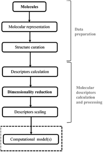
Molecular similarity analysis (Stumpfe and Bajorath 2011) is one of the alternative cheminformatics methods to forensic drug analysis presently available (Bero et al. 2017; Krasowski and Ekins 2014). The assumption made by the molecular similarity analysis approach is that molecules with similar structures are more likely to have the same experimental properties (Grisoni, Consonni, and Todeschini 2018). Furthermore, this approach requires informative and discriminative molecular descriptors (Todeschini and Consonni 2010) that provide information about the molecular features for the target candidate molecule in the chemical database (Grisoni, Consonni, and Todeschini 2018; Todeschini and Consonni 2010). One disadvantage related to cheminformatics is the high dimensionality of molecular descriptors (Lavecchia 2015). The principal steps of molecular descriptors generation are depicted in Figure 1 (Grisoni, Consonni, and Todeschini 2018). According to the figure, dimensionality reduction is required immediately after descriptors generation to remove redundant and irrelevant information in the original molecular descriptors. This is to provide the best subset of descriptors for computational models such as similarity search analysis (Krasowski et al. 2009), quantitative structure-activity relation (QSAR) (Cerruela García et al. 2019; Panwala et al. 2017) analysis, and machine learning approaches in cheminformatics (Khan and Roy 2018; Lo et al. 2018; Mitchell B.O. 2014; Vo et al. 2020).

Figure 1. Principal steps of molecular descriptors generation for computational models

Feature selection is one of the popular dimensionality reduction approaches. The goal of this approach is to select a small subset of relevant features by removing redundancy, irrelevant and noisy features (Idakwo et al. 2018; Shahlaei 2013). In cheminformatics, descriptor selection is essential for several reasons including (Goodarzi, Dejaegher, and Heyden 2012): (i) increase the computational model interpretability and understandability by fewer descriptors; (ii) avoid overfitting by eliminating noisy and redundant descriptors (iii) produce a fast and effective computational model, and (iv) prevents the activity cliff.

Swarm Intelligence (SI) algorithms undertook feature selection (Brezočnik, Fister, and Podgorelec 2018; Nayar, Ahuja, and Jain 2019; Nguyen-Tri et al. 2020) and proven as a technique that can solve NP-hard combinatorial search problems such as the selection of an optimal feature subset from high-dimensional features (Albrecht 2006). SI algorithms are gaining prominence in feature selection because of their ability to escape local optima, simplicity and, easier of implementation (Ismail Sayed et al. 2017).

The initial intention of the SI algorithm is to solve the continuous optimization problem. Researchers have taken advantage of the flexibility of this algorithm to implement it in feature selection problems by proposing the binary version of it. One common way to convert the continuous solution to a binary solution in the SI algorithm is to use a transfer function. Families of the transfer function in the literature include the S-shaped (Hussien et al. 2019), V-shaped (Hussien, Houssein, and Hassanien 2017), time-varying (M. Mafarja et al. 2018), and quadratic (Algamal et al. 2020; Too, Abdullah, and Saad 2019a) transfer functions.

In cheminformatics, the implementation of SI-based feature selection approach to molecular descriptors has been shown in several works using particle swarm optimization (PSO) (Khajeh, Modarress, and Zeinoddini-Meymand 2013), firefly algorithm (FA) (Fouad et al. 2018), salps swarm algorithm (SSA) (Hussien, Hassanien, and Houssein 2017), grasshopper optimization algorithm (GOA) (Algamal et al. 2020), etc.

No-Free-Lunch (NFL) theorem for search and optimization derived by Wolpert and Macready (1997) has become the motivation of this research to confirm the universality of binary particle swarm optimization (BPSO) algorithm, binary whale optimization algorithm (WOA), and binary manta ray foraging optimization (MRFO) algorithm as descriptors selection approach for ATS drug classification problem. The performance of the algorithms is evaluated using seven performance evaluation criteria. The optimally selected feature subset was tested using the k-Nearest Neighbor (k-NN) classifier.

The remainder of this paper is organized as follows: the next section reveals the necessary material and methods used in the study. The section is comprised of several subsections that briefly describe the overview of the 3D-ELMI molecular descriptors dataset, followed by the theoretical explanations regarding BPSO, BWOA, and BMRFO algorithms and their application in feature selection. Section 3 displays and discusses the obtained empirical results of feature selection and classification by BPSO, BWOA, and BMRFO algorithms implementation. Finally, Section 4 concludes with some recommendations for future work.

Materials and Methods

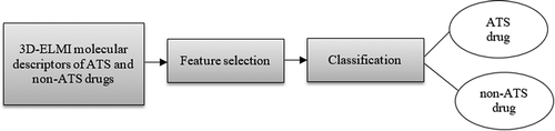
The process flow of the proposed ATS drug classification system is presented in Figure 2. Firstly, the existing 3D-ELMI molecular descriptors dataset is obtained. Next, feature selection methods, BPSO, BWOA, and BMRFO are used for selecting the optimal feature subset. The selected feature subset is then inputted to the k-Nearest Neighbor (k-NN) algorithm to perform the classification process.

Figure 2. Process flow of the proposed ATS drug classification system

Overview of 3D Exact Legendre Moment Invariants (3D-ELMI) Molecular Descriptors Dataset

Before performing the ATS drug classification, the molecular descriptors of ATS and non-ATS drugs must be generated before and as input to the feature selection techniques and the classifier. Though, this study directly utilized the available dataset produced using the novel 3D-ELMI molecular descriptors introduced by Pratama (2017) on 7190 samples of drug molecules (3595 ATS drugs and 3595 non-ATS drugs). These descriptors generate a one-dimensional vector of 1185 independent features to describe the 3D molecular structure of each drug molecule. Table 1 outlines the attributes contain in the dataset.

Table 1. Attributes description

Attribute	Attribute type	No. of attribute	Description
Molecule id	String	1	Molecule id refers to the reference id of the drug molecule in the original database.
Featuren	Numeric (real numbers)	1185	Moment invariants value calculated using 3D-ELMI molecular descriptors to represent the drug 3D molecular structure. n is feature number takes value from 1 to 1185.
Class	Nominal {0,1}	1	0: non-ATS and 1: ATS

The Binary Version of Swarm-Intelligence Algorithms

The solutions in the feature selection problem are restricted to the binary values of 0 and 1. Similar to native algorithms, in binary version algorithms, the search agents (solutions) repetitively updating their locations to any position in the search space following the leading search agent found so far. The transfer function is one way that can be applied to convert the real position of the search agent to binary values (Mirjalili and Lewis 2013). Search agents are forced to travel in a binary space by transfer function with probability definition which updates each element in the search agent to 1 (selected) or 0 (not selected). This study adopted an S-shaped transfer function, the sigmoid function that has been implemented in these studies (Al-Tashi et al. 2019; Eid 2018; Too, Abdullah, and Saad 2019b). Equation 1(1) $S\left(x\right)=\frac{1}{1+e^{-10\left(x-0.5\right)}}$(1) shows the mathematical formulation of the sigmoid transfer function (Al-Tashi et al. 2019; Panwala et al.):

(1) $S\left(x\right)=\frac{1}{1+e^{-10\left(x-0.5\right)}}$(1)

where $x$ is the current position (continuos value) of the search agent. Then, $x$ is updated as in Equation 2(2) $x=\left\{\begin{array}{c}1,ifS\left(x\right)\ge rand\\ 0,otherwise\end{array}\right.$(2) (Kennedy and Eberhart 1997) based on the probability value $S\left(x\right)$ obtained in Equation 1(1) $S\left(x\right)=\frac{1}{1+e^{-10\left(x-0.5\right)}}$(1) :

(2) $x=\left\{\begin{array}{c}1,ifS\left(x\right)\ge rand\\ 0,otherwise\end{array}\right.$(2)

$rand$ is a random number in the [0,1] interval.

Binary Particle Swarm Optimization Algorithm

An algorithm that simulates bird flocking was proposed by Kennedy and Eberhart, (1995) named Particle Swarm Optimization (PSO). The population PSO is made of n particles with two properties speed (velocity) and position. Kennedy and Eberhart (1997) introduced the initial binary PSO (BPSO) to solve the binary optimization problems. For finding the best solution, the particle moves around the search space finding the global maximum or minimum based on its own experience and knowledge (Gupta, Baghel, and Iqbal 2018). The optimal position of each particle is recognized as Pbest while Gbest is the global best solution in the population. The velocity of a particle is updated in each iteration t as in Equation 3(3) $v_i^d\left(t+1\right)=w\left(t\right)\times v_i^d\left(t\right)+c1\times r1\times (Pbes{t}_i^d\left(t\right)-x_i^d\left(t\right))+c2\times r2\times (Gbes{t}_i^d\left(t\right)-x_i^d\left(t\right))$(3) :

(3) $v_i^d\left(t+1\right)=w\left(t\right)\times v_i^d\left(t\right)+c1\times r1\times (Pbes{t}_i^d\left(t\right)-x_i^d\left(t\right))+c2\times r2\times (Gbes{t}_i^d\left(t\right)-x_i^d\left(t\right))$(3)

where x, v and i represent the position, velocity, order of the particle in the population. d denotes the search space dimension, w indicates the inertia weight, c1 and c2 represent the acceleration coefficients, r1 and r2 are the random vectors in [0, 1], and t the iteration number.

For BPSO, the sigmoid transfer function is applied to the velocity to convert to a probability value:

(4) $S\left(v_i^d\left(t+1\right)\right)=\frac{1}{1+e^{-10\left(v_i^d\left(t+1\right)-0.5\right)}}$(4)

Finally, the new position is updated using Equation 5(5) $x_i^d\left(t+1\right)=\left\{\begin{array}{c}1,ifS\left(v_i^d\left(t+1\right)\right)\ge rand\\ 0,otherwise\end{array}\right.$(5) .

(5) $x_i^d\left(t+1\right)=\left\{\begin{array}{c}1,ifS\left(v_i^d\left(t+1\right)\right)\ge rand\\ 0,otherwise\end{array}\right.$(5)

Binary Whale Optimization Algorithm

An algorithm that is inspired by the hunting mechanism of humpback whales called bubble-net foraging was proposed by Mirjalili and Lewis (2016) known as a whale optimization algorithm (WOA). The binary WOA (BWOA) is firstly proposed by Zamani and Nadimi-Shahraki (2016) for feature selection in disease diagnosis. In the initial stage, the WOA algorithm will assume the target prey as the best search agent that is near to the optimum. Then, other whales (search agents) will update their positions based on the best search agent. WOA swarming behavior is simulated in mathematical formulations below:

(6) $D=\left|C{X}^{\ast }\left(t\right)-X\left(t\right)\right|$(6)

(7) $X\left(t+1\right)=\hspace{0.17em}{X}^{\ast }\left(t\right)-AD$(7)

where $t$ is the iteration number. $X\left(t\right)$denotes the candidate search agent at iteration number $t$ and $X^{\ast }\left(t\right)$ indicate as the best search agent (prey) so far. $A$ and $C$ are coefficient numbers mathematically formulated by Equation 8(8) $A=2ar+a$(8) and Equation 9(9) $C=2r$(9) . D indicates the distance vector between whale (search agent) and prey (best search agent). In each iteration $X^{\ast }\left(t\right)$ is updated when there is a better solution.

(8) $A=2ar+a$(8)

(9) $C=2r$(9)

where r is a random vector in [0, 1]. The value of a linearly decreases from 2 to 0 over iterations. The bubble-net behavior of humpback whales in the exploitation phase is designed based on two mechanisms: (1) Shrinking encircling of prey: The humpback move in a shrinking encircling along a spiral-shaped path toward the prey by decreasing a variable value in Equation 8(8) $A=2ar+a$(8) . $A$ is a random value in the interval $\left(-a,a\right)$,

(10) $a=2-t\frac{2}{MaxIter}$(10)

where $t$ indicates the iteration number and $MaxIter$ is the maximum number of iterations. (2) Spiral updating position: A logarithmic spiral function is used to imitate the helix-shaped movement of humpback whales between the candidate whale (search agent) $X\left(t\right)$, and the prey (best search agent), $X^{\ast }\left(t\right)$ so far. This procedure is mathematically expressed in Equation 12(12) $X\left(t+1\right)=D^{\ast }{e}^{bl}cos\left(2\pi l\right)+X^{\ast }\left(t\right),$(12) .

(11) $D^{\ast }=\left|X^{\ast }\left(t\right)-X\left(t\right)\right|,$(11)

(12) $X\left(t+1\right)=D^{\ast }{e}^{bl}cos\left(2\pi l\right)+X^{\ast }\left(t\right),$(12)

where $b$ is a constant and $l$ is a random number in the range between −1 and 1.

During the optimization phase, an assumption of 50% probability is used to choose between these two mechanisms to update the whales’ position. The mathematical formulation to model this behavior is established as follows:

(13) $\begin{array}{rl}& X\left(t+1\right)=\left\{\begin{array}{c}{X}^{\ast }\left(t\right)-AD,ifp0.5,\\ D^{\ast }{e}^{bl}cos\left(2\pi l\right)+X^{\ast }\left(t\right),ifp\ge 0.5,\end{array}\right.\end{array}$(13)

where $p$ is a random number in $\left(0,1\right).$

In the exploration phase, the hunt for prey is conducted at random. Contradicting with the exploitation phase, a search agent position is updated following a randomly chosen search agent. A contains a random value that is either greater than 1 or less than −1. These values will urge the search agent to move far away from the best whale. With this mechanism and $\left|A\right|>1$, it allows WOA to perform a global search in overcoming the problem of the local optima. Equation 15(15) $X\left(t+1\right)=X_{rand}-A\hspace{0.17em}D$(15) describes the mathematical formulation:

(14) $D=\left|\mathrm{C}{X}_{rand}-X\right|$(14)

(15) $X\left(t+1\right)=X_{rand}-A\hspace{0.17em}D$(15)

where $X_{rand}$ indicates a whale that is randomly chosen from the current population.

For BWOA, the sigmoid transfer function is applied to the solution position to convert to a probability value:

(16) $S\left(X\left(t+1\right)\right)=\frac{1}{1+e^{-10\left(X\left(t+1\right)-0.5\right)}}$(16)

Finally, the new position is updated using Equation 17(17) $X\left(t+1\right)=\left\{\begin{array}{c}1,ifS\left(X\left(t+1\right)\right)\ge rand\\ 0,otherwise\end{array}\right.$(17) .

(17) $X\left(t+1\right)=\left\{\begin{array}{c}1,ifS\left(X\left(t+1\right)\right)\ge rand\\ 0,otherwise\end{array}\right.$(17)

Binary Manta Ray Foraging Optimization Algorithm

Manta ray foraging optimization (MRFO) algorithm is recently proposed by Zhao, Zhang, and Wang (2020) that inspired by manta ray foraging. MRFO comprises three foraging behaviors which are chain foraging, cyclone foraging, and somersault foraging. Manta rays dine on plankton, small fish, and small shrimp. The early binary MRFO (BMRFO) algorithm was proposed by Ghosh et al. (2021) using transfer functions.

The three MRFO foraging strategies’ mathematical formulation is described in the following: (1) Chain foraging: Manta rays swim in an orderly line toward the position of the observed plankton. If former manta rays (search agents) missed plankton, other subsequent manta rays (search agents) will scoop it. Highly concentrated plankton at a respective position signifies a better position. The chain foraging mathematical modeling is represented in Equation 12(12) $X\left(t+1\right)=D^{\ast }{e}^{bl}cos\left(2\pi l\right)+X^{\ast }\left(t\right),$(12) :

(18) $x_i^d\left(t+1\right)=\left\{\begin{array}{c}{x}_i^d\left(t\right)+r\left(x_{best}^d\left(t\right)-x_i^d\left(t\right)\right)+\alpha \left(x_{best}^d\left(t\right)-x_i^d\left(t\right)\right)ifi=1\\ x_i^d\left(t\right)+r\left(x_{i-1}^d\left(t\right)-x_i^d\left(t\right)\right)+\alpha \left(x_{best}^d\left(t\right)-x_i^d\left(t\right)\right)ifi=2,\dots ,N\end{array}\right.$(18)

(19) $\alpha =2r\sqrt{\left|log\left(r\right)\right|}$(19)

where $x_i^d\left(t\right)$ denotes the position of the search agent. $i$ is the order of the manta ray, d denotes the search space dimension, t the iteration number, and r is a random vector in [0, 1]. α represents the weight coefficient. The position with the highest plankton concentration is denoted as $x_{best}^d$ and it is assumed as the best solution in MRFO. (2) Cyclone foraging: Manta ray (search agent) moves spirally toward plankton and swim to other manta rays (search agent) in the head-to-tail link. The mathematical model of the spiral-shaped movement is defined as follows:

(20) $x_i^d\left(t+1\right)=\left\{\begin{array}{c}{x}_{best}^d\left(t\right)+r\left(x_{best}^d\left(t\right)-x_i^d\left(t\right)\right)+\beta \left(x_{best}^d\left(t\right)-x_i^d\left(t\right)\right)ifi=\\ x_{best}^d\left(t\right)+r\left(x_{i-1}^d\left(t\right)-x_i^d\left(t\right)\right)+\beta \left(x_{best}^d\left(t\right)-x_i^d\left(t\right)\right)ifi=2,\dots ,N\end{array}\right.$(20)

(21) $\beta =2e^{r_1\frac{T-t+1}{T}}sin\left(2\pi r_1\right)$(21)

where $T$ is the maximum number of iterations, $\beta$ is a weight coefficient and $r_1$ is a random vector in [0, 1]. A new random position that is far from the current best one is assigned to each search agent to promote an extensive global search in MRFO. Equation 23(23) $x_i^d\left(t+1\right)=\left\{\begin{array}{c}{x}_{rand}^d\left(t\right)+r\left(x_{rand}^d\left(t\right)-x_i^d\left(t\right)\right)+\beta \left(x_{rand}^d\left(t\right)-x_i^d\left(t\right)\right)ifi=1\\ x_{rand}^d\left(t\right)+r\left(x_{i-1}^d\left(t\right)-x_i^d\left(t\right)\right)+\beta \left(x_{rand}^d\left(t\right)-x_i^d\left(t\right)\right)ifi=2,\dots ,N\end{array}\right.$(23) express the mathematical model:

(22) $x_{rand}^d\hspace{0.17em}=L{b}^d+rU{b}^d-L{b}^d$(22)

(23) $x_i^d\left(t+1\right)=\left\{\begin{array}{c}{x}_{rand}^d\left(t\right)+r\left(x_{rand}^d\left(t\right)-x_i^d\left(t\right)\right)+\beta \left(x_{rand}^d\left(t\right)-x_i^d\left(t\right)\right)ifi=1\\ x_{rand}^d\left(t\right)+r\left(x_{i-1}^d\left(t\right)-x_i^d\left(t\right)\right)+\beta \left(x_{rand}^d\left(t\right)-x_i^d\left(t\right)\right)ifi=2,\dots ,N\end{array}\right.$(23)

where $x_{rand}^d$indicates the search agent random position, $L{b}^d$ and $U{b}^d$ are lower and upper boundaries and d denotes the dimension of the search space. (3) Somersault foraging: The position of the best plankton found so far is used as a pivot. Each search agent swims back and forth around the pivot and somersault to a new position. Equation 24(24) $x_i^d\left(t+1\right)=x_i^d\left(t\right)+S\left(r_2{x}_{best}^d-r_3{x}_i^d\left(t\right)\right),i=1,\hspace{0.17em}2,\dots ,\hspace{0.17em}N\hspace{0.17em}$(24) shows the mathematical model:

(24) $x_i^d\left(t+1\right)=x_i^d\left(t\right)+S\left(r_2{x}_{best}^d-r_3{x}_i^d\left(t\right)\right),i=1,\hspace{0.17em}2,\dots ,\hspace{0.17em}N\hspace{0.17em}$(24)

where $S$ is the somersault factor, $r_2$ and $r_3$ are random numbers in [0, 1].

For BMRFO, the sigmoid transfer function is applied to the solution position to convert to a probability value:

(25) $S\left(x_i^d\left(t+1\right)\right)=\frac{1}{1+e^{-10\left(x_i^d\left(t+1\right)-0.5\right)}}$(25)

Finally, the new position is updated using Equation 26(26) $x_i^d\left(t+1\right)=\left\{\begin{array}{c}1,ifS\left(x_i^d\left(t+1\right)\right)\ge rand\\ 0,otherwise\end{array}\right.$(26) .

(26) $x_i^d\left(t+1\right)=\left\{\begin{array}{c}1,ifS\left(x_i^d\left(t+1\right)\right)\ge rand\\ 0,otherwise\end{array}\right.$(26)

Application of BPSO, BWOA, and BMRFO for Feature Selection

Maximize the classification accuracy and minimizing the feature size are the two main goals of the feature selection technique (M. Mafarja and Mirjalili 2018). Since a wrapper-based feature selection technique is used, the evaluation process includes a learning algorithm for classification. The k-Nearest Neighbor (k-NN) algorithm (Altman 1992) with the Euclidean distance matric where k = 5 is used in this study (Eid 2018; M. Mafarja et al. 2019b). The k-NN algorithm is chosen because of its satisfactory results and speedy processing.

An optimal feature subset should have a minimal classification error rate and a small-size feature subset. A fitness function for feature selection is designed to balance the two criteria. The fitness function for evaluating the solutions is presented in Equation 27(27) $\downarrow Fitness=\alpha {\gamma }_R\left(D\right)+\beta \frac{\left|R\right|}{\left|C\right|}$(27) :

(27) $\downarrow Fitness=\alpha {\gamma }_R\left(D\right)+\beta \frac{\left|R\right|}{\left|C\right|}$(27)

where${\gamma }_R\left(D\right)$ is the classification error rate. $\left|R\right|$ denotes the length of the selected feature subset, and $\left|C\right|$ indicates a total number of features in the original dataset. Parameters $\alpha ,$ and $\beta$ correspond to the importance of classification quality and feature subset length where $\alpha \in \left[1,0\right]$ and $\beta =\left(1-\alpha \right)$ (Emary, Zawbaa, and Hassanien 2016a; Sharawi et al. 2017). In this study, the classification metric is the most important thus we set $\alpha$ to 0.99 (Hussien et al. 2019; Houssein et al. 2020; M. M. Mafarja and Mirjalili 2019).

Experimental Dataset Preparation

The molecule id attribute is excluded during the experiment (refer to Table 1). In all experiments, the hold-out validation was employed where 80% of samples were chosen randomly as training set and the remaining 20% of samples are used as the testing set. This partitioning was also applied in several works in the literature (M. Mafarja et al. 2019a; M. Mafarja and Mirjalili 2018).

Parameter Settings

Table 2 shows the specific parameter settings that are utilized in binary SI algorithms as feature selectors. For a fair comparison, this study has fixed the number of iteration (t) to 70 for all algorithms. On the other hand, the number of search agents (n) was chosen at 5. Problem dimension (d) is the same as the number of original features in the dataset, in this case, is 1185.

Table 2. BPSO, BWOA, and BMRFO parameters setting

Parameter	Value
BPSO, BWOA, BMRFO
No. of runs, M	15
Problem dimension, d	1185
No. of search agents, n	5
No. of iterations, t	70
$\alpha$ parameter in the fitness function	0.99
$\beta$ parameter in the fitness function	0.01
BPSO
Cognitive factor, c1	2
Social factor, c2	2
Maximum velocity, Vmax	6
Minimum velocity, Vmin	−6
Inertia weight, w	0.9 to 0.4
BWOA
$\vec{a}$ in WOA	2 to 0
b	1
BMRFO
Somersault factor, S	2

Evaluation Criteria

The experimental results are viewed as the mean of metrics obtained from 15 independent runs (M) to obtain statistically valid results. To ensure the consistency and statistical significance of the obtained results, the data partitioning is repeated in each independent run. All algorithms are implemented and analyzed in Matlab R2019b and executed on an Intel Core i7-6700 machine, 3.40 GHz CPU with Windows 10 operating system, and 16 GB of RAM.

The following evaluation metrics are employed in (Emary, Zawbaa, and Hassanien 2016b; Hussien, Hassanien, and Houssein 2017) are implemented and recorded from the testing data in each run:

(28) $Mean\mathrm{\_}Accuracy=\frac{1}{M}\sum _{j=1}^M\frac{1}{N}\sum _{i=1}^{N}Match\left(C_i,L_i\right),$(28)

where $M$ is the total runtime, $N$ indicates the total instance in the testing set, $C_i$ is predicted label by the classifier for instance i, $L_i$ is the actual class label, for instance, i, and $Match$ is a function that validates whether $C_i$ and $L_i$ are the same by outputting 1 if identical and 0 vice versa.

(29) $Best\mathrm{\_}fitness=\begin{array}{c}M\\ min\\ i=1\end{array}{g}_{\ast }^i$(29)

(30) $Worst\mathrm{\_}fitness=\begin{array}{c}M\\ max\\ i=1\end{array}{g}_{\ast }^i,$(30)

(31) $Mean\mathrm{\_}fitness=\frac{1}{M}\sum _{i=1}^M{g}_{\ast }^i,$(31)

where M is the total runtime$,g_{\ast }^i$ has the optimal solution resulted from a runtime i. Best_fitness indicates the smallest fitness value achieved at the maximum iteration by each algorithm over runtime. Worst_fitness denotes the largest fitness value achieved by each algorithm over runtime. $Mean\mathrm{\_}fitness$ signifies the average fitness value achieved by each algorithm over runtime. The algorithm that achieved the minimal value of Best_fitness, Worst_fitness, and Mean_fitness is considered as having good convergence.

(32) $\mathrm{S}\mathrm{t}\mathrm{a}\mathrm{n}\mathrm{d}\mathrm{a}\mathrm{r}\mathrm{d}\mathrm{\_}\mathrm{d}\mathrm{e}\mathrm{v}\mathrm{i}\mathrm{a}\mathrm{t}\mathrm{i}\mathrm{o}\mathrm{n}=\sqrt{\frac{1}{M-1}}{\sum }^{{\left(g_{\ast }^i-Mean\mathrm{\_}fitness\right)}^2},$(32)

(33) $\mathrm{M}\mathrm{e}\mathrm{a}\mathrm{n}\mathrm{\_}\mathrm{F}\mathrm{e}\mathrm{a}\mathrm{t}\mathrm{u}\mathrm{r}\mathrm{e}\mathrm{\_}\mathrm{S}\mathrm{e}\mathrm{l}\mathrm{e}\mathrm{c}\mathrm{t}\mathrm{e}\mathrm{d}\mathrm{\_}\mathrm{S}\mathrm{i}\mathrm{z}\mathrm{e}=\frac{1}{M}\sum _{i=1}^M\frac{size\left(g_{\ast }^i\right)}{D},$(33)

where size ($g_{\ast }^i$) is the size of the selected feature subset, and D is the number of features in the original data set.

(34) $\mathrm{M}\mathrm{e}\mathrm{a}\mathrm{n}\mathrm{\_}\mathrm{C}\mathrm{o}\mathrm{m}\mathrm{p}\mathrm{u}\mathrm{t}\mathrm{a}\mathrm{t}\mathrm{i}\mathrm{o}\mathrm{n}\mathrm{\_}\mathrm{T}\mathrm{i}\mathrm{m}\mathrm{e}=\frac{1}{M}\sum _{i=1}^{M}Runtim{e}_i,$(34)

where $Runtim{e}_i$, is the computation time in second at runtime $i$.

Results and Discussion

Table 3 presented the average of the minimum, maximum, mean, standard deviation of fitness values and their mean computation time to converge. The best result for each method is highlighted in bolded text. From the results, BPSO is seen to achieve the lowest fitness value. Instead, BWOA achieves the lowest maximum and mean fitness values. To reflect and compare the optimization accuracy and convergence rate of each algorithm more intuitively, the average convergence curves of the three algorithms are plotted, as shown in Figure 3. Based on the curves in Figure 3, it is observed that BMRFO shows the fastest convergence at early iteration and starts to remain stagnance at iteration 30 and onwards. Instead, BPSO and BWOA continue to converge, and leading BMRFO at iteration 40 resultant in the lowest fitness achieved by BPSO and BWOA in second.

Table 3. Results show the mean of minimum fitness (Min), maximum fitness (Max), mean fitness (Mean), standard deviation (Std), and computation time (CT) obtained by BPSO, BWOA, and BMRFO algorithms

Algorithm	Min	Max	Mean	Std	CT
BPSO	0.18451	0.26298	0.19746	0.01585	34.51
BWOA	0.18650	0.23819	0.19535	0.01152	402.51
BMRFO	0.18997	0.24396	0.19536	0.00945	1015.03

Figure 3. Convergence curves of BPSO, BWOA, and BMRFO algorithms

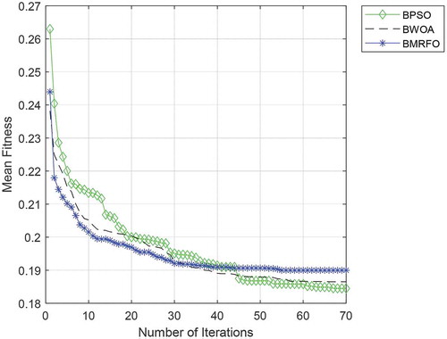
Moreover, the results of the computation time of each binary algorithm displayed that BPSO was also the fastest algorithm to converge with the shortest computation time. BPSO was able to attain the lowest fitness within 34.51 seconds compared to BPSO and BMRFO with 402.51 seconds and 1015.03 seconds. By observing the standard deviation result in Table 3, the standard deviation obtained for all the algorithms is low and shows that the average fitness results deviate less. This suggests that these algorithms have provided consistent and robust performance over different runs. Despite that BMRFO has the lowest standard deviation, it also achieved the high minimum fitness that demonstrated BMRFO is suffered from premature convergence and stagnation behaviors.

The experimental results that quantify the mean accuracy and mean selected feature size attained by BPSO, BWOA, and BMRFO are listed in Table 4. By examining the result in Table 4, it can be seen that BWOA has obtained a comparable mean classification accuracy with BPSO, whereas BMRFO scored the lowest accuracy. On the other hand, BPSO is shown to have selected the smallest set of relevant features followed by BWOA and BMRFO.

Table 4. Results show the means of accuracy an selected feature size of BPSO, BWOA and BMRFO algorithms

Algorithm	Mean Accuracy (%)	Mean Selected Feature Size
All	62.63%	1185
BPSO	81.39%	37
BWOA	81.41%	293.3
BMRFO	81.11%	350.15

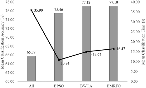
Table 4 also stated the mean classification accuracy of 62.63% is attained by k-NN when all features in the dataset were utilized. Mean classification accuracy increased approximately 30% after the feature selection technique is implemented by using BPSO, BWOA, and BMRFO. In terms of the number of features, Table 4 shows the feature reduction of 96.88%, 75.25%, and 70.45% from the original dataset was obtained by BPSO, BWOA, and BMRFO. The smaller and optimal feature subset can enrich the learning and understandability of the classifier model to provide a good prediction. In addition, it may also accelerate the classifier learning and prediction processes.

Table 5 outlines the results of mean classification accuracies from using different classifiers. Additionally, the time taken by each classifier to learn and predict the class label is also specified in Table 6. The results from Table 5 and Table 6 were averaged and displayed in Figure 4. The results confirmed that BWOA has achieved a better classification performance of 77.12% with only utilizing 24.75% of selected relevant features from the original dataset among others. Besides, BMRFO is in second place with a comparable mean accuracy of 77.10%. BPSO is seen has gained the lowest mean accuracy from the table. It indicates that too small features may be caused information loss and disadvantages to some classifiers. Overall, it is proven that the feature selection technique can improve the classifier efficiency in terms of prediction and speed when significant features are provided.

Table 5. Mean classification accuracies with different classifiers

Classifier	All	BPSO	BWOA	BMRFO
k-NN	62.63%	81.39%	81.41%	81.11%
SVM (linear)	77.98%	78.62%	79.83%	79.88%
SVM (RBF)	67.24%	80.93%	82.00%	82.02%
SVM (Polynomial)	50.29%	66.40%	79.51%	79.75%
SVM(Gaussian)	67.46%	80.95%	81.99%	82.00%
NB (Normal)	68.37%	71.15%	68.57%	68.23%
NB (Kernel)	66.53%	68.77%	66.52%	66.73%

Table 6. Mean classification time in seconds with different classifiers

Classifier	All	BPSO	BWOA	BMRFO
k-NN	3.12	0.07	0.69	0.82
SVM (linear)	64.44	1.91	3.43	3.94
SVM (RBF)	22.40	0.97	3.56	4.18
SVM (Polynomial)	40.96	69.03	69.90	74.84
SVM(Gaussian)	22.00	0.95	3.61	4.27
NB (Normal)	0.39	0.02	0.10	0.10
NB (Kernel)	98.01	2.92	23.49	27.16

Figure 4. The average mean classification accuracies and times by all classifiers

Our overall research finding reveals the importance of feature selection in molecular descriptors in the cheminformatics domain that always deals with an enormous volume of chemical data. Specifically, this research has recommended an alternative in drug forensic toxicology which combined the image processing technique as a feature extractor to form molecular descriptors from previous research and feature selection technique and machine learning classifiers in the current research that able to reduce time, cost, and effort in identifying existing and new ATS drugs through their 3D molecular structure. The authors believe that further improvement to this proposed method may yield more promising results in the future.

Conclusion and Future Works

This paper has proved the advantages of implementing BPSO, BWOA, and new BMRFO algorithms in the wrapper feature selection methods to improve the ATS drug classification task. The 3D-ELMI molecular descriptors dataset is utilized to validate the performance of these three algorithms in selecting significant features without degrading the classification accuracy. Experimental results quantified that BWOA is proficient as a feature selector where it manages to produce a small and relevant feature subset for different classifiers to provide good classification. In the future, this research plan to tune the BWOA parameters such as the number of search agents and the number of fitness iteration. Furthermore is to examine BWOA with other families of transfer functions. Finally is to evaluate the dataset with other available SI-based algorithms in the literature.

Acknowledgments

This work was supported by Fundamental Research Grant Scheme [FRGS/1/2020/FTMK-CACT/F00461] from the Ministry of Higher Education, Malaysia.

Disclosure statement

The authors do not have any conflict of interest.

References

- Albrecht, A. A. 2006. Stochastic local search for the feature set problem, with applications to microarray data. Applied Mathematics and Computation 183 (2):1148–64. doi:https://doi.org/10.1016/j.amc.2006.05.128.
- Algamal, Z. Y., M. K. Qasim, M. H. Lee, and H. T. M. Ali. 2020. QSAR model for predicting neuraminidase inhibitors of influenza a viruses (H1N1) based on adaptive grasshopper optimization algorithm. SAR and QSAR in Environmental Research 1–12. doi:https://doi.org/10.1080/1062936X.2020.1818616.
- Al-Tashi, Q., S. J. A. Kadir, H. M. Rais, S. Mirjalili, and H. Alhussian. 2019. Binary optimization using hybrid grey wolf optimization for feature selection. IEEE Access 7:39496–508. doi:https://doi.org/10.1109/ACCESS.2019.2906757.
- Altman, N. S. 1992. An Introduction to kernel and nearest-neighbor nonparametric regression. American Statistician 46 (3):175–85. doi:https://doi.org/10.1080/00031305.1992.10475879.
- Bero, S. A., A. K. Muda, Y. H. Choo, N. A. Muda, and S. F. Pratama. 2017. Similarity measure for molecular structure: a brief review. Journal of Physics: Conference Series 892:1. doi:https://doi.org/10.1088/1742-6596/892/1/012015.
- Brandt, S. D., and P. V. Kavanagh. 2017. Addressing the challenges in forensic drug chemistry. Drug Testing and Analysis 9 (3):342–46. doi:https://doi.org/10.1002/dta.2169.
- Brezočnik, L., I. Fister, and V. Podgorelec. 2018. Swarm intelligence algorithms for feature selection: A review. Applied Sciences (Switzerland) 8:9. doi:https://doi.org/10.3390/app8091521.
- Cerruela García, G., J. Pérez-Parras Toledano, A. de Haro García, and N. García-Pedrajas. 2019. Filter feature selectors in the development of binary QSAR models. SAR and QSAR in Environmental Research 30 (5):313–45. doi:https://doi.org/10.1080/1062936X.2019.1588160.
- Chung, H., and S. Choe. 2019. Amphetamine-Type stimulants in drug testing. Mass Spectrometry Letters 10 (1):1–10. doi:https://doi.org/10.5478/MSL.2019.10.1.1.
- Drummer, O. H., and D. Gerostamoulos. 2013. Forensic drug analysis. Forensic Drug Analysis 1–125. doi:https://doi.org/10.4155/9781909453371.
- Eid, H. F. 2018. Binary whale optimisation: An effective swarm algorithm for feature selection. International Journal of Metaheuristics 7 (1):67. doi:https://doi.org/10.1504/IJMHEUR.2018.091880.
- Emary, E., H. M. Zawbaa, and A. E. Hassanien. 2016a. Binary ant lion approaches for feature selection. Neurocomputing 213:54–65. doi:https://doi.org/10.1016/j.neucom.2016.03.101.
- Emary, E., H. M. Zawbaa, and A. E. Hassanien. 2016b. Binary grey wolf optimization approaches for feature selection. Neurocomputing 172:371–81. doi:https://doi.org/10.1016/j.neucom.2015.06.083.
- Fouad, M. A., E. H. Tolba, M. A. El-Shal, and A. M. El Kerdawy. 2018. QSRR modeling for the chromatographic retention behavior of some β-Lactam antibiotics using forward and firefly variable selection algorithms coupled with multiple linear regression. Journal of Chromatography A 1549:51–62. doi:https://doi.org/10.1016/j.chroma.2018.03.042.
- Ghosh, Kushal Kanti, Ritam Guha, Suman Kumar Bera, Neeraj Kumar, and Ram Sarkar. 2021. “S-Shaped versus V-Shaped Transfer Functions for Binary Manta Ray Foraging Optimization in Feature Selection Problem.” Neural Computing & Application. https://doi.org/https://doi.org/10.1007/s00521-020-05560–9
- Goodarzi, M., B. Dejaegher, and Y. V. Heyden. 2012. Feature selection methods in QSAR Studies. Journal of AOAC International 95 (3):636–51. doi:https://doi.org/10.5740/jaoacint.SGE_Goodarzi.
- Grisoni, F., V. Consonni, and R. Todeschini. 2018. Impact of molecular descriptors on computational models. Computational Chemogenomics, ed. J. B. Brown, vol. 1825, 1st ed., 171–209. New York: Humana Press. doi:https://doi.org/10.1007/978-1-4939-8639-2.
- Gupta, S. L., A. S. Baghel, and A. Iqbal. 2018. Threshold controlled binary particle swarm optimization for high dimensional feature selection. International Journal of Intelligent Systems and Applications 10 (8):75–84. doi:https://doi.org/10.5815/ijisa.2018.08.07.
- Harper, L., J. Powell, and E. M. Pijl. 2017. An overview of forensic drug testing methods and their suitability for harm reduction point-of-care services. Harm Reduction Journal 14 (1):1. doi:https://doi.org/10.1186/s12954-017-0179-5.
- Houssein, E. H., M. E. Hosney, M. Elhoseny, D. Oliva, W. M. Mohamed, and M. Hassaballah. 2020. Hybrid harris hawks optimization with cuckoo search for drug design and discovery in chemoinformatics. Scientific Reports 10 (1):1–22. doi:https://doi.org/10.1038/s41598-020-71502-z.
- Hussien, A. G., A. E. Hassanien, and E. H. Houssein. 2017. “Swarming behaviour of salps algorithm for predicting chemical compound activities.” 2017 IEEE 8th International Conference on Intelligent Computing and Information Systems, ICICIS 2017 2018-Janua (Icicis): 315–20. https://doi.org/10.1109/INTELCIS.2017.8260072.
- Hussien, A. G., A. E. Hassanien, E. H. Houssein, S. Bhattacharyya, and M. Amin. 2019. S-Shaped binary whale optimization algorithm for feature selection. advances in intelligent systems and computing, vol. 727. Springer Verlag. doi:https://doi.org/10.1007/978-981-10-8863-6_9.
- Hussien, A. G., E. H. Houssein, and A. E. Hassanien. 2017. “A binary whale optimization algorithm with hyperbolic tangent fitness function for feature selection.” 2017 IEEE 8th International Conference on Intelligent Computing and Information Systems, ICICIS 2017 2018 Janua (Icicis): 166–72. https://doi.org/10.1109/INTELCIS.2017.8260031.
- Idakwo, G., J. Luttrell, M. Chen, H. Hong, Z. Zhou, P. Gong, and C. Zhang. 2018. A review on machine learning methods for in silico toxicity prediction. Journal of Environmental Science and Health - Part C Environmental Carcinogenesis and Ecotoxicology Reviews 36 (4):169–91. doi:https://doi.org/10.1080/10590501.2018.1537118.
- Ivy, C. F., A. H. Lewin, S. Wayne Mascarella, H. H. Seltzman, and P. Anantha Reddy. 2012. Designer drugs: A medicinal chemistry perspective. Annals of the New York Academy of Sciences 1248 (1):18–38. doi:https://doi.org/10.1111/j.1749-6632.2011.06199.x.
- Kennedy, J., and R. C. Eberhart. 1997. Discrete binary version of the particle swarm algorithm. Proceedings of the IEEE International Conference on Systems, Man and Cybernetics 5:4104–08. doi:https://doi.org/10.1109/icsmc.1997.637339.
- Kennedy, James, and Russel Eberhart. 1995. “Particle Swarm Optimization.” In Proceedings of the IEEE International Conference on Neural Networks, 1942–48. Perth, Australia: IEEE. https://doi.org/10.1002/9780470612163
- Khajeh, A., H. Modarress, and H. Zeinoddini-Meymand. 2013. Modified particle swarm optimization method for variable selection in QSAR/QSPR studies. Structural Chemistry 24 (5):1401–09. doi:https://doi.org/10.1007/s11224-012-0165-1.
- Khan, P. M., and K. Roy. 2018. Current approaches for choosing feature selection and learning algorithms in Quantitative Structure–Activity Relationships (QSAR). Expert Opinion on Drug Discovery 13 (12):1075–89. doi:https://doi.org/10.1080/17460441.2018.1542428.
- Krasowski, M. D., M. G. Siam, A. F. Manisha Iyer, S. G. Pizon, S. Ekins, and S. Ekins. 2009. Chemoinformatic methods for predicting interference in drug of abuse/toxicology immunoassays. Clinical Chemistry 55 (6):1203–13. doi:https://doi.org/10.1373/clinchem.2008.118638.
- Krasowski, M. D., and S. Ekins. 2014. Using cheminformatics to predict cross reactivity of ‘designer drugs’ to their currently available immunoassays. Journal of Cheminformatics 6 (1):1–13. doi:https://doi.org/10.1186/1758-2946-6-22.
- Lavecchia, A. 2015. Machine-learning approaches in drug discovery: methods and applications. Drug Discovery Today 20 (3):318–31. doi:https://doi.org/10.1016/j.drudis.2014.10.012.
- Liu, L., S. E. Wheeler, R. Venkataramanan, J. A. Rymer, A. F. Pizon, M. J. Lynch, and K. Tamama. 2018. Newly emerging drugs of abuse and their detection methods: An ACLPS critical review. American Journal of Clinical Pathology 149 (2):105–16. doi:https://doi.org/10.1093/AJCP/AQX138.
- Lo, Y. C., S. E. Rensi, W. Torng, and R. B. Altman. 2018. Machine learning in chemoinformatics and drug discovery. Drug Discovery Today 23 (8):1538–46. doi:https://doi.org/10.1016/j.drudis.2018.05.010.
- Mafarja, M., I. Aljarah, A. A. Heidari, H. Faris, P. Fournier-Viger, L. Xiaodong, and S. Mirjalili. 2018. Binary dragonfly optimization for feature selection using time-varying transfer functions. Knowledge-Based Systems 161 (August):185–204. doi:https://doi.org/10.1016/j.knosys.2018.08.003.
- Mafarja, M., I. Aljarah, H. Faris, A. I. Hammouri, A. M. Al-Zoubi, and S. Mirjalili. 2019a. Binary grasshopper optimisation algorithm approaches for feature selection problems. Expert Systems with Applications 117:267–86. doi:https://doi.org/10.1016/j.eswa.2018.09.015.
- Mafarja, M., I. Jaber, S. Ahmed, and T. Thaher. 2019b. Whale optimisation algorithm for high-dimensional small-instance feature selection. International Journal of Parallel, Emergent and Distributed Systems 0:1–17. doi:https://doi.org/10.1080/17445760.2019.1617866.
- Mafarja, M., and S. Mirjalili. 2018. Whale optimization approaches for wrapper feature selection. Applied Soft Computing Journal 62:441–53. doi:https://doi.org/10.1016/j.asoc.2017.11.006.
- Mafarja, M. M., and S. Mirjalili. 2019. Hybrid binary ant lion optimizer with rough set and approximate entropy reducts for feature selection. Soft Computing 23 (15):6249–65. doi:https://doi.org/10.1007/s00500-018-3282-y.
- Mirjalili, S., and A. Lewis. 2013. S-Shaped versus V-Shaped transfer functions for binary particle swarm optimization. Swarm and Evolutionary Computation 9:1–14. doi:https://doi.org/10.1016/j.swevo.2012.09.002.
- Mirjalili, S., and A. Lewis. 2016. The whale optimization algorithm. Advances in Engineering Software 95:51–67. doi:https://doi.org/10.1016/j.advengsoft.2016.01.008.
- Mitchell, B. O., and B. O. John. 2014. Machine learning methods in chemoinformatics. Wiley Interdisciplinary Reviews: Computational Molecular Science 4 (5):468–81. doi:https://doi.org/10.1002/wcms.1183.
- Nayar, N., S. Ahuja, and S. Jain. 2019. Swarm intelligence for feature selection: A review of literature and reflection on future challenges. In Advances in Data and Information Sciences, vol. 39, 211–21. Lecture No. Springer Nature Singapore Pte Ltd. doi: https://doi.org/10.1007/978-981-13-0277-0_18.
- Nguyen-Tri, P., P. Ghassemi, P. Carriere, S. Nanda, A. A. Assadi, and D. D. Nguyen. 2020. Recent applications of advanced atomic force microscopy in polymer science: A review. Polymers 12 (5):1–28. doi:https://doi.org/10.3390/POLYM12051142.
- Pratama, S. F. 2017. Three-dimensional exact legendre moment invariants for amphetamine-type stimulants molecular structure representation. Universiti Teknikal Malaysia Melaka, Malaysia.
- Reschly-Krasowski, J. M., and M. D. Krasowski. 2018. a difficult challenge for the clinical laboratory: Accessing and interpreting manufacturer cross-reactivity data for immunoassays used in urine drug testing. Academic Pathology 5:237428951881179. doi:https://doi.org/10.1177/2374289518811797.
- Sayed, I., A. D. Gehad, A. E. Hassanien, and J.-S. Pan. 2017. Breast cancer diagnosis approach based on meta-heuristic optimization algorithm inspired by the bubble-net hunting strategy of whales. In ed., J.-S. Pan, J. Chun-Wei Lin, C.-H. Wang, and X. H. Jiang. Advances in Intelligent Systems and Computing. Proceedings of the tenth international conference on genetic and evolutionary computing. vol. 536, 306–313. Cham: Springer International Publishing. doi:https://doi.org/10.1007/978-3-319-48490-7.
- Shahlaei, M. 2013. Descriptor selection methods in quantitative structure-activity relationship studies: A review study. Chemical Reviews 113 (10):8093–103. doi:https://doi.org/10.1021/cr3004339.
- Sharawi, M., H. M. Zawbaa, E. Emary, and E. Hossamzawbaagmailcom. 2017. “Feature selection approach based on whale optimization algorithm.” In 2017 Ninth International Conference on Advanced Computational Intelligence (ICACI), Doha, 163–68. IEEE.
- Stumpfe, D., and J. Bajorath. 2011. Similarity Searching. Wiley Interdisciplinary Reviews: Computational Molecular Science 1 (2):260–82. doi:https://doi.org/10.1002/wcms.23.
- Todeschini, R., and V. Consonni. 2010. Molecular Descriptors for Chemoinformatics. Molecular Descriptors for Chemoinformatics. doi:https://doi.org/10.1002/9783527628766.
- Too, J., A. R. Abdullah, and N. M. Saad. 2019a. A new quadratic binary harris hawk optimization for feature selection. Electronics (Switzerland) 8 (10):1–27. doi:https://doi.org/10.3390/electronics8101130.
- Too, J., A. R. Abdullah, and N. M. Saad. 2019b. Hybrid binary particle swarm optimization differential evolution-based feature selection for EMG signals classification. Axioms 8 (3):3. doi:https://doi.org/10.3390/axioms8030079.
- Vo, A. H., T. R. Van Vleet, R. R. Gupta, M. J. Liguori, and M. S. Rao. 2020. An overview of machine learning and big data for drug toxicity evaluation. Chemical Research in Toxicology 33 (1):20–37. doi:https://doi.org/10.1021/acs.chemrestox.9b00227.
- Wolpert, D. H., and W. G. Macready. 1997. No Free Lunch Theorems. IEEE Transactions On Evolutionary Computation 1 (1):67–82. doi:https://doi.org/10.1109/4235.585893.
- Zamani, H., and N.-S. Mohammad-Hossein. 2016. Feature selection based on whale optimization algorithm for diseases diagnosis. International Journal of Computer Science and Information Security 14 (9):1243–47.
- Zhao, W., Z. Zhang, and L. Wang. 2020. Manta ray foraging optimization: An effective bio-inspired optimizer for engineering applications. Engineering Applications of Artificial Intelligence 87 October 2019:103300. doi:https://doi.org/10.1016/j.engappai.2019.103300