Machine Learning Based Power Estimation for CMOS VLSI Circuits

ABSTRACT

Nowadays, machine learning (ML) algorithms are receiving massive attention in most of the engineering application since it has capability in complex systems modeling using historical data. Estimation of power for CMOS VLSI circuit using various circuit attributes is proposed using passive machine learning-based technique. The proposed method uses supervised learning method, which provides a fast and accurate estimation of power without affecting the accuracy of the system. Power estimation using random forest algorithm is relatively new. Accurate estimation of power of CMOS VLSI circuits is estimated by using random forest model which is optimized and tuned by using multiobjective NSGA-II algorithm. It is inferred from the experimental results testing error varies from 1.4% to 6.8% and in terms of and Mean Square Error is 1.46e-06 in random forest method when compared to BPNN. Statistical estimation like coefficient of determination (R) and Root Mean Square Error (RMSE) are done and it is proven that random Forest is best choice for power estimation of CMOS VLSI circuits with high coefficient of determination of 0.99938, and low RMSE of 0.000116.

Introduction

Due to recent development in VLSI technology million of transistors are fabricated in a single chip. Increase in number of transistor and operating speed in a chip and speed due which ultimately increase the power consumption and has become a crucial concern in submicron technology. In VLSI circuits, power estimation at an earlier stage is highly needed, because it has a major impact on the reliability of VLSI circuits. Under this condition, at the higher levels of design abstraction average power estimation before a chip manufacturing is very much essential to calculate power budget and to take necessary steps to reduce power consumption. The objective of the proposed work is to develop less complex and low cost power estimation technique, which can be alternative solution to the conventional techniques like SPICE circuit simulation which are based on the assumption of predefined empirical equations(2) $RMSE=\sqrt{\frac{{\sum }_{I=1}^N\left(Y_I^O\right.{\left.-Y_I^C\right)}^2}{N}}$(2) .

Literature Overview

Power dissipation of the circuit depends on the inputs, frequency, and operating voltage. Simulation and nonsimulation-based method are two main categories to estimate average power. Amuru and Abbas (2020) proposed an estimation technique for leakage power, delay in standard CMOS/FinFET digital cells. Bhanja and Ranganathan (2003) explained about switching activity estimation using Bayesian Networks considering both in internal nodes and inputs. Burch et al. (1993) and Saxena, Najm, and Hajj (1997) proposed simulation-based method, which includes Monte Carlo approach. Estimate the power for combinational and sequential circuits was discussed by Buyuks and Najm (2006) and Kozhaya and Najm (2001). Adaptive neuro fuzzy application to power estimation was discussed by Govindaraj and Ramesh (2018). Kirei and Topa (2019) explained about estimation of power in CMOS integrated circuits with discrete time filters in which filter of various complexities are considered and power and area estimates are obtained. Ligang Hou, Zheng, and Wu (2006) proposed a method using Levenberg-Marquardt function to estimate power using Neural Network. Murugavel et al. (2002) proposed a method using Least square estimation to estimate average power which minimize MSE through each iteration when compared to Monte Carlo approach. Under Probabilistic class, Burch et al. (1993) devised an algorithm to propagate of transition density values from the primary input to the primary output. BPNN and Radial Basis Function Neural Network (RBFNN)-based power estimation of ISCAS’89 sequential Benchmark circuits have been performed by Ramanathan, Surendiran, and Vanathi (2013). Only two training functions Traingdm and Traingdx were used for analysis out of eleven different training algorithms available in MATLAB tool. Omnia et al. (2016) discussed about estimation of dynamic power consumption using circuit nodes and logic picture for CMOS combinational logic circuits Shaw Halwai (2020) proposed a method to estimate power dissipation of phase detector circuit. Nasser et al. (2021) developed a model to estimate power of digital components, using Artificial Neural Networks (ANNs), the technology used as target technology is Application Specific Integrated Circuit (ASIC). Survey of various power estimation is summarized by Nasser et al. (2020).

Chao Chen et al. (2020) discussed about classification of neural activities, brain–computer interfaces, classification of finger gestures during motor execution and imagery. Estimation of Cumulative Pollution Index of Insulator Strings Leakage using random forest was proposed by De Santos and Sanz-Bobi (2020). Metal Oxide Surge Arrester-based surface condition identification using random forest is done by Das, Dalai, and Chatterjee (2020). Impedance estimation in power system using machine learning is proposed by Liang and Zheng (2019). Pilarski et al. (2012), Seyedzadeh, Glesk, and Roper (2018) Peng, Lima, and Teakles (2017) developed human and robot integration, Monitoring of electric power grid and building energy management systems using machine learning. Air pollution measurement using Machine Learning Techniques was discussed by Srivastava and Singh (2018). A perspective on machine learning in turbulent flows was discussed by Sandeep Pandey, Schumacher, and Sreenivasan (2020) similarly Pradhan and Chawla (2020) proposed Medical Internet of things using machine learning algorithms for lung cancer detection.

Machine Learning models will discover the relationship between input variables and outputs of interest from the system being studied or learn from measured data or simulated data that represents the physical problem. Nowadays, machine learning (ML) models are receiving enormous attention in most of the fields due to their capability in modeling complex systems using historical data. The use of data-driven models have been successfully demonstrated in applications demanding for real-time estimation of the targets values. The proposed work employs an Random forest algorithm which has the ability to estimate the power of CMOS VLSI circuits, without the knowledge on actual circuit structure and interconnections. The Random forest algorithm results are compared with BPNN results. Error percentage for BPNN and Random Forest is calculated to find the deviation from actual power to predicted power in which Random Forest outperforms BPNN.

Experimental Setup

Training and Testing Data

The database used for training and testing the BPNN and random forest network is obtained from the literature (Hou, Zheng, and Wu 2006) which is shown in Tables 1 and 2. BPNN network is trained by using database of 20 Benchmark ISCAS’89 sequential circuits and 5 the same circuits are used for testing purpose. The training and testing consists of attributes such as considered for sequential circuits are number of inputs, outputs, D flip-flops, inverters, total number of gates, AND gates, NAND gates, OR gates, and NOR gates. The database for training and testing has been taken from reference (Hou, Zheng, and Wu 2006; Murugavel et al. 2002) in that the power dissipated corresponding to a set of input patterns was observed in SIS (SIS is an interactive tool for synthesis and optimization of sequential circuits) by (i) sampling, (ii) zero delay, (iii) uniform distribution for switching at the nodes, and (iv) clock frequency of 20 MHz and power supply of 5. The results of the database (Hou, Zheng, and Wu 2006; Murugavel et al. 2002) are compared with the Monte Carlo method .

Table 1. ISCAS’89 benchmark circuit data set for training BPNN/RF (Hou, Zheng, and Wu 2006)

Benchmark circuit	GATE	AND	INV	NOR	NAND	OR	DFF	IN	OUT	Monte Carlo Simulation power in mw.
S208	66	21	38	16	15	14	8	10	1	0.00698
S298	75	31	44	19	9	16	14	3	6	0.00912
S349	104	44	57	31	19	10	15	9	11	0.01856
S420	160	49	78	34	29	28	16	18	1	0.00903
S444	119	13	62	34	58	14	21	3	6	0.01172
S713	139	94	254	0	28	17	19	35	23	0.03743
S820	256	76	33	66	54	60	5	18	19	0.02831
S838	288	105	158	70	57	56	32	34	1	0.01292
S953	311	49	84	112	114	36	29	16	23	0.02458
S1238	428	134	80	57	125	112	18	14	14	0.06347
S1423	490	197	167	92	64	137	74	17	5	0.07181
S1488	550	350	103	0	0	200	6	8	19	0.05648
S1494	558	354	89	0	0	204	6	8	19	0.06018
S5378	1004	0	1775	765	0	239	179	35	49	0.23357
S9234	2027	955	3570	113	528	431	228	19	22	0.28004
S13207	2573	1114	5378	98	849	512	669	31	121	0.35404
S15850	3448	1619	6324	151	968	710	597	14	87	0.51991
S35932	12204	4032	3861	0	7020	1152	1728	35	320	1.22048
S38417	8709	4154	13470	2279	2050	226	1636	28	106	1.14518
S38584	11448	5516	7805		12	278	1452	2621	1185	1.87987

Table 2. ISCAS’89 benchmark circuit data set for testing BPNN/RF (Hou, Zheng, and Wu 2006)

Benchmark circuit	GATE	AND	INV	NOR	NAND	OR	DFF	IN	OUT
S344	101	44	59	30	18	9	15	9	11
S382	99	11	59	34	30	24	21	3	6
S386	118	83	41	0	0	35	6	7	7
S400	106	11	58	34	36	25	21	3	6
S641	107	90	272	0	4	13	19	35	24

Proposed Random Forest-Based Power Estimation

In the proposed method, a Random Forest (RF) model is preferred due to its ability to predict multiple output values Simultaneously. Until one record remain as subset RF divide the records in to smaller and smaller subset since RF is an ensemble of randomized decision trees. The nodes and leaf nodes are called as inner and final sets. RF needs a number of numbers of hyper-parameters to be set and to achieve maximum accuracy, these parameters are tuned as per simulated data to get accurate power estimation of CMOS VLSI Circuits . The constructed model is trained and tested using 10-fold cross-validation. Implementation is done using Python programming language, and the proposed work is carried out on a Computer with Intel Core i7-6700 3.4 GHz CPU, 16GB RAM.

The work flow of BPNN and RF Algorithm is shown in Figure 1 in which training is done by using two third of system dataset and testing is done using one-third of system data set (Harris 1994), training algorithm and training parameters are properly chosen to estimate power.

Figure 1. Workflow of BPNN and RF algorithm

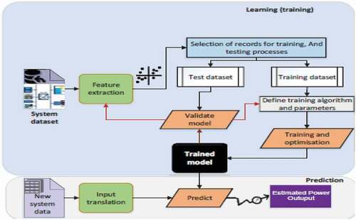
Maximum depth in RF model is varied from 10 to 15, number of trees from 150 to 750, neighbor order is 1. The parameter neighbor order gives the relationship between adjacent subcells. The neighbor condition can be measured by the neighbor-order parameter.

Steps Involved in RF Algorithm

1. From the training dataset k data points are pick in random.

2. Using the k data points a decision tree associated with data points is constructed.

3. Step 1 and 2 are repeated to build N number N of trees .

4. By using each one of tree in N – tree, output value Y corresponding to a new data point is determined and average of all predicted Y values is calculated and final Y value is identified.

Power Estimation Using BPNN

The method consists of the following steps:

• Construction of neural network

• Training phase

• Testing phase

Construction of Neural Network

A back-propagation neural network is constructed with four-layer feed-forward. First layer is set with ‘linear’ transfer function and ‘tansig’ function is chosen for remaining layers. BPNN network Parameters such as learning rate, epoch, hidden layer and momentum constant are varied for different training algorithms such as Traingd, Trainscg, Traingda, Trainbfg, Trainrp, Trainoss, Traingdx, Trainsgf, Traingdm, Traincgp, and Traincgb. The data base of sequential circuits consists of nine attributes, therefore number of inputs for the network is considered as nine. The generalized architecture of BPNN is shown in Figure 2.

Figure 2. Architecture of BPNN

Training Phase

1: Two-third of the input vectors from ISCAS’89 benchmark circuits database are extracted and to train the BPNN (Harris 1994).

2: Normalization is done for input vectors and their corresponding target vectors. Since the the hidden layers has tan-sigmoidal activation function normalization is done between the −1 to +1.

3: The BPNN network is trained with the normalized input vectors and their corresponding normalized target vectors.

Testing Phase

1: One-third of the input vectors from ISCAS’89 benchmark circuits database are used for testing (Harris 1994).

2: Before testing, the parameters used for input test vectors are normalized.

3:Outputs vectors are generated for these normalized test input vectors by the BPNN network.

4: Original value is obtained from reverse normalization process.

Results and Discussion

Number of neurons at the input side is based on the number of input attributes used for training the neural network. The number of attributes is varied from 9 to 7 by eliminating OR gates and AND gates in the input. In few cases reducing the attributes gave best result, for example traincgf and traincgp training functions with 7 input attributes perform better than 9 input. BPNN is a feed-forward back propagation type neural network consists of Learning rate, Momentum constant, activation function and training algorithm as four important parameter. Momentum constant is varied between 0.1 and 0.9, number of epochs is varied between 150 and 2700, hidden layer neurons are selected between 10 and 17, 0.3 and 0.8 is the range of variation for learning rate for 11 different training algorithm and activation functions are chosen as tansig and logsig The stopping criteria are selected using extensive MATLAB simulation as shown in Table 3. Table 4 gives Regression results comparison of ISCAS’89 benchmark circuits using BPNN for 11 different training functions.

Table 3. Stopping criteria for BPNN

Neural network parameter	Range of variation
Momentum constant	0.1–0.9
No. of neurons in hidden layer	10–17
Learning rate	0.3–0.8
No. of epochs	150–2700

Table 4. Regression results comparison of ISCAS’89 benchmark circuits using BPNN

Training function	Layer size	Epochs	Number of input attributes	Slope	Y-intercept	Regression value	Deviation in %	MSE
Trainscg	9:15:15:1	253	9	1	−0.0034	0.9999	0.01	6.254E-05
Traincgp	7:15:15:1	300	9	1.8	−0.025	0.9988	0.12	0.02672
Traincgb	9:16:15:1	100	9	1.7	−0.023	0.9993	0.07	0.02403
Trainoss	8:14:15:1	600	9	0.99	0.0017	0.9991	0.09	0.01924
Trainbfg	9:15:15:1	500	9	1.4	−0.016	0.9993	0.07	0.01793
Traingd	9:15:15:1	750	9	1.8	−0.027	0.9940	0.6	0.014096
Traingdm	8:13:14:1	400	9	0.015	0.0016	0.9920	0.8	0.02485
Traingdx	8:14:15:1	225	9	0.34	0.018	0.9979	0.21	0.01602
Traincgf	7:15:15:1	256	9	1.1	−0.0036	0.9990	0.1	0.00528
Traingda	9:15:14:1	500	9	0.58	0.011	0.9956	0.44	0.025339
Trainrp	8:16:15:1	250	9	1	−1.6x10^−5	0.9998	0.02	0.06346

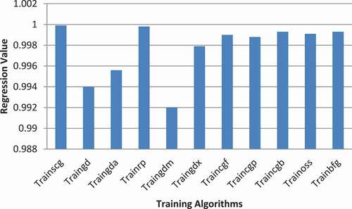
Trainscg training function which is based on conjugate gradient algorithm provides better results for sequential circuits when compared to other training algorithms. From the regression analysis it is found that the results for ISCAS’89 sequential benchmark circuits deviates from ideal power by 0.01%–0.8%. The trainscg training function gives the minimum regression value among other 11 training algorithms. Trainscg under conjugate gradient category is best suited for power estimation for sequential circuits for a layer size of 9:15:15:1 with 9 inputs and 253 epochs. Regression results comparison of ISCAS ’89 circuits with the previous literature using BPNN is shown in Table 5. Since the existing method uses ISCAS’89 circuits we have chosen the same circuit as indicated in Tables 1 and 2. From the Figure 3, it is inferred that trainscg predicts power very close to power estimator tool than remaining training algorithm.

Table 5. Regression results comparison of ISCAS ’89 circuits with the existing methods using BPNN

Training function	Input	Activation function	Epochs	Layer size	Y-intercept (B)	Slope (M)	Regression (R)	Regressiion value Deviation in % (1-R)*100
Trainlm (LigangHou)	9	Tansig	2139	6:15:15:1	−.000963	0.915	0.994	0.6
Traingdx (Ramanathan)	8	Logsig	225	7:14:15:1	2.77 E-04	1.044	0.9982	0.18
Traingdx (Ramanathan)	8	Tansig	265	8:13:15:1	0.0051	1.045	0.9999	0.01
Trainlm (Ligang Hou)	9	Tan sig	878	9:15:15:1	−.000882	0.464	0.753	24.7
Trainscg	9	Tansig	253	9:15:15:1	−0.0034	1	0.9999	0.01
Trainbfg	9	Tansig	500	9:15:15:1	−0.016	1.4	0.9993	0.07

Figure 3. ISCAS’89 benchmark circuits regression result comparison using BPNN for 11 training algorithms

Predicted power output and Mean square error of ISCAS’89 Bench mark circuit is shown in Table 6, which is obtained by comparing actual circuit output with neural network, and random forest predicted output. MSE is calculated for both BPNN and RF. MSE of RF is 1.46E-06 whereas BPNN is 3.842E-05 this shows ML models discover relationships between input variables and outputs of interest from the system being studied, learn from measured or simulated data. Figure 4 Comparison of ISCAS’89 benchmark circuits Actual output with RF and BPNN predicted output.

Table 6. Mean square error of ISCAS’89 benchmark circuits using BPNN/RF

Benchmark circuits	Actual output	BPNN (MSE)		Random forest (MSE)
		Predicted output	Squared error	Predicted output	Squared error
S344	0.01846	0.0193	7.056E-07	0.0182	6.76E-08
S382	0.01046	0.0176	5.098E-05	0.0103	2.56E-08
S386	0.01628	0.0182	3.686E-06	0.0153	9.604E-07
S400	0.01065	0.01087	4.84E-08	0.0104	6.25E-08
S641	0.03629	0.0246	0.0001367	0.0338	6.2E-06
Mean Square Error			3.842 E-05		1.46E-06

Figure 4. Comparison of ISCAS’89 benchmark circuits actual output with RF and BPNN-predicted output

Performance Analysis of BPNN and RF

Training and testing prediction error is calculated using equation (1)(1) $Error\mathrm{\%}=\frac{A-BX100}{A}$(1)

(1) $Error\mathrm{\%}=\frac{A-BX100}{A}$(1)

where A is the actual value and B is the predicted output value by testing the network.

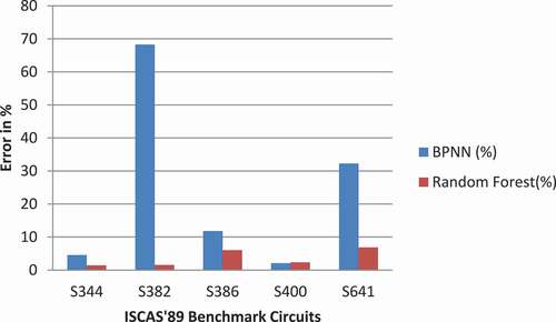
Prediction error comparison of BPNN with RF is reported in Table 7. It is infer that RF prediction error is varying from 1.4% to 6.8% but BPNN prediction error is varying from 4.5% to 68.2% . RF prediction error is less than BPNN because it can deal with regression and classification problems of multiclass, small sample data, and without data pre processing procedures.

Table 7. Error calculation for BPNN and RF

Benchmark circuit	BPNN error in (%)	Random forest error in (%)
S344	4.55038	1.408451
S382	68.26	1.529637
S386	11.7936	6.019656
S400	2.06573	2.347418
S641	32.21273	6.861394

Figure 5 gives comparison of Prediction error of RF and BPNN in which RF outperforms BPNN.

Figure 5. Comparison of prediction error of RF and BPNN

Performance of RF and BPNN network can be determined by doing statistical analysis such Root Mean Square Error (RMSE) and Coefficient of determination (R) which is given below in Equation (2)(2) $RMSE=\sqrt{\frac{{\sum }_{I=1}^N\left(Y_I^O\right.{\left.-Y_I^C\right)}^2}{N}}$(2) – (3(3) $R=\frac{{\sum }_{I=1}^N\left(Y_I^O\right.-\left.Y_{\hspace{0.17em}}^O\right)\left(Y_I^C\right.-\left.Y_{\hspace{0.17em}}^C\right)}{\sqrt{{\sum }_{I=1}^N\left(Y_I^O\right.-{\left.Y_{\hspace{0.17em}}^O\right)}^2{\sum }_{I=1}^N\left(Y_I^C\right.-{\left.Y_{\hspace{0.17em}}^C\right)}^2}}$(3) ).

(2) $RMSE=\sqrt{\frac{{\sum }_{I=1}^N\left(Y_I^O\right.{\left.-Y_I^C\right)}^2}{N}}$(2)

(3) $R=\frac{{\sum }_{I=1}^N\left(Y_I^O\right.-\left.Y_{\hspace{0.17em}}^O\right)\left(Y_I^C\right.-\left.Y_{\hspace{0.17em}}^C\right)}{\sqrt{{\sum }_{I=1}^N\left(Y_I^O\right.-{\left.Y_{\hspace{0.17em}}^O\right)}^2{\sum }_{I=1}^N\left(Y_I^C\right.-{\left.Y_{\hspace{0.17em}}^C\right)}^2}}$(3)

where Y^O is the mean of observed value, Y_I^O is the observed value Y^C is the mean of calculated value, and Y_I^C is the calculated value. RMSE is used as a measure to find the difference between predicted values and measured values. RMSE can be used as an indicator of model accuracy or precision. A good network /model should has RMSE value low, or as close to zero.

The coefficient of determination R determines a linear correlation between measured values and values simulated by the model, optimal value is 1. RMSE and R for BPNN and ANFIS is shown in Table 8, from the table we infer that RMSE of RF is less when compared to BPNN and R value of RF is very close to 1. Considering these measures, the RF model achieves high accuracy for power estimation.

Table 8. Statistical analysis test on BPNN and RF

Parameter	BPNN	Random forest
RMSE	0.0004499	0.000116
R	0.84696	0.99938

Conclusion

In this paper, a supervised learning method to estimate the Power of CMOS VLSI circuits is presented. The proposed RF model is an alternative approach to the conventional techniques like SPICE circuit simulation, which are based on the assumption of predefined empirical equations and arbitrary parameters. The results of RF are highly accurate and the details of circuit structure and interconnections are not required. Random Forest is less computationally than BPNN. A random forest for a decision tree will give a different interpretation but with better performance on the other hand BPNN requires much more data for the result to be effective. Hence, RF with exclusive characteristics appears as a better choice for estimation of power in CMOS VLSI circuits. It is proven that by using statistical estimation like coefficient of determination and Root Mean Square Error (RMSE), RF performs well for power estimation application with high coefficient of determination of 0.99938 and low RMSE of 0.000116.

Disclosure Statement

Author don’t have any conflict of interest in submitting the paper to this journal.

References

- Amuru, M. S. A., and Z. Abbas 2020. An efficient gradient boosting approach for PVT aware estimation of leakage power and propagation delay in CMOS/FinFET digital cells. IEEE International Symposium on Circuits and Systems (ISCAS), Sevilla, 1–5. doi: https://doi.org/10.1109/ISCAS45731.2020.9180600.
- Bhanja, S., and N. Ranganathan. 2003. Switching activity estimation of VLSI circuits using Bayesian networks. IEEETransactions on Very Large Scale Integration Systems 11 (4):558–67. doi:https://doi.org/10.1109/TVLSI.2003.816144.
- Burch, R., F. N. Najm, P. Yang, and T. N. Trick. 1993. A Monte Carlo approach for power estimation. IEEE Transactions on Very Large Scale Integration Systems 2 (1):63–71. doi:https://doi.org/10.1109/92.219908.
- Buyuks, M. K., and F. N. Najm. 2006. Early power estimation for VLSI circuits. IEEE Transactions on Computer Aided Design of Integrated Circuits and Systems 24 (7):1076–88. doi:https://doi.org/10.1109/TCAD.2005.850904.
- Chen, B., P. Chen, A. N. Belkacem, L. Lu, R. Xu, W. Tan, P. Li, Q. Gao, D. Shin, C. Wang, et al. 2020. Neural activities classification of left and right finger gestures during motor execution and motor imagery. Brain-Computer Interfaces 1–11. doi:https://doi.org/10.1080/2326263X.2020.1782124.
- Das, A. K., S. Dalai, and B. Chatterjee 2020. Cross stockwell transform aided random forest based surface condition identification of metal oxide surge arrester employning leakage current signal. 2020 IEEE Region 10 Symposium (TENSYMP), 1775–78. doi: https://doi.org/10.1109/TENSYMP50017.2020.9230802.
- De Santos, H., and M. Á. Sanz-Bobi. 2020. A cumulative pollution index for the estimation of the leakage current on insulator strings. IEEE Transactions on Power Delivery 35 (5):2438–46. doi:https://doi.org/10.1109/TPWRD.2020.2968556.
- Govindaraj, V., and J. Ramesh. 2018. Adaptive neuro fuzzy inference system-based power estimation method for CMOS VLSI circuits. International Journal of Electronics, Taylor and Francis 105 (3):398–411.
- Harris, C. J. 1994. Advances in intelligent control. Boca Raton, FL: CRC Press. ISBN 9780748400669.
- Hou, L., L. Zheng, and W. Wu 2006. Neural network based VLSI power estimation. 2006 8th International Conference on Solid-State and Integrated Circuit Technology Proceedings. doi:https://doi.org/10.1109/icsict.2006.306506
- Kirei, S. C. F., and M. D. Topa 2019. Power and area estimation of discrete filters in CMOS integrated circuits. Signal Processing: Algorithms, Architectures, Arrangements, and Applications (SPA), Poznan, Poland, 67–70, doi: https://doi.org/10.23919/SPA.2019.8936762.
- Kozhaya, J. N., and F. N. Najm. 2001. Power estimation for large sequential circuits. IEEE Transactions on Very Large Scale Integration Systems 9 (2):400–07. doi:https://doi.org/10.1109/ICCAD.1997.643581.
- Liang, H. G., and T. Zheng. 2019. Real-time impedance estimation for power line communication. IEEE Access 7:88107–15. doi:https://doi.org/10.1109/ACCESS.2019.2925464.
- Murugavel, A. K., N. Ranganathan, R. Chandramouli, and S. Chavali. 2002. Least-square estimation of average power in digital CMOS circuits. IEEE Transactions on Very Large Scale Integration Systems 10 (1):55–58. doi:https://doi.org/10.1109/92.988730.
- Nasser, Y., J. Lorandel, J.-C. Prevotet, and M. Hélard. 2021. RTL to transistorlevel power modelling and estimation techniques for FPGA and ASIC: A survey. IEEE Transac-tions on Computer-Aided Design of Integrated Circuits and Systems 40 (3):479–93. doi:https://doi.org/10.1109/TCAD.2020.3003276.
- Omnia S. Fadl, Mohamed F. Abu-Elyazeed, Mohamed B. Abdelhalim, Hassanein H. Amer, Ahmed H. Madian(2016). Accurate dynamic power estimation for CMOS combinational logic circuits with real gate delay model. Journal of Advanced Research 7 (1) 89-94. ISSN 2090-1232. https://doi.org/https://doi.org/10.1016/j.jare.2015.02.006
- Pandey, S., J. Schumacher, and K. R. Sreenivasan. 2020. A perspective on machine learning in turbulent flows. Journal of Turbulence 21 (9–10):567–84. doi:https://doi.org/10.1080/14685248.2020.1757685.
- Peng, H., A. R. Lima, and A. Teakles. 2017. Evaluating hourly air quality forecasting in Canada with nonlinear updatable machine learning methods. Air Quality, Atmosphere, & Health 10 (2):195–211, March. doi:https://doi.org/10.1007/s11869-016-0414-3.
- Pilarski, M. R. D., T. Degris, J. P. Carey, and R. S. Sutton 2012. Dynamic switching and real-time machine learning for improved human control of assistive biomedical robots. 4th IEEE RAS & EMBS International Conference on Biomedical Robotics and Biomechatronics (BioRob), Rome, Italy, June, 296–302.
- Pradhan, K., and P. Chawla. 2020. Medical Internet of things using machine learning algorithms for lung cancer detection. Journal of Management Analytics 7 (4):591–623. doi:https://doi.org/10.1080/23270012.2020.1811789.
- Ramanathan, P., B. Surendiran, and P. T. Vanathi. 2013. Power estimation of benchmark circuits using artificial neural networks. Pensee Journal 75 (9):427–33.
- Saxena, V., F. N. Najm, and I. N. Hajj 1997. Monte-Carlo approach for power estimation in sequential circuits. European Design and Test conference, (ED&TC 97), March 17–20, 416–20. doi:https://doi.org/10.1109/EDTC.1997.582393.
- Seyedzadeh, F. P. R., I Glesk, and M. Roper. 2018. Machine learning for estimation of building energy consumption and performance: A review. Visualization in Engineering 6:5. doi:https://doi.org/10.1186/s40327-018-0064-7.
- Shaw Halwai, K. K. 2020. Estimation of power and delay of CMOS phase detector and phase-frequency detector using nano dimensional MOS transistor. IEEE VLSI Device Circuit and System (VLSI DCS), Kolkata, India, 294–98. doi: https://doi.org/10.1109/VLSIDCS47293.2020.9179921.
- Srivastava, S. S., and A. P. Singh 2018.Estimation of air pollution in Delhi using machine learning techniques. International Conference on Computing, Power and Communication Technologies (GUCON), 304–09. doi: https://doi.org/10.1109/GUCON.2018.8675022.
- Yehya Nasser, C. S., J.-C. Pr´evotet, T. Fanni, F. Palumbo, M. H´elard, and L. Raffo. 2020. NeuPow: A CAD methodology for high level power estimation based on machine learning. ACM Transactions on Design Automation of Electronic Systems 25 (5):1–29. doi: https://doi.org/10.1145/3388141.