Neural Network Architecture Selection Using Particle Swarm Optimization Technique

ABSTRACT

Finding the best structure of ANN to minimize errors, the processing and the search time is one of the main objectives in the AI field. In order to achieve prediction with a high degree of accuracy in a short time, an enhanced PSO-based selection technique to determine the optimal configuration for the artificial neural network has been proposed in this paper. To design the neural network to minimize processing time, search time and maximize the accuracy of prediction, it is necessary to identify hyperparameter values with precision. PSO with 2-D search space has been employed to select the best hyperparameters in order to construct the best neural network where PSO is used as a decision-making model and ANN is used as a learning model. The suggested technique was used to select the optimal number of the hidden layer and the number of units per hidden layer. The proposed technique was evaluated using a chemical dataset. The result of testing the proposed technique displayed high prediction accuracy with MSE equal to 3.9% and the relative error between the expected output and actual target is less than 1.6%. The results of the comparison of the proposed technique with the ANN showed thatthe proposed approach could predict output with an infinitesimal error, outperforming the existing ANN model in terms of error ratio.

Introduction

Due to the significant need for data prediction in different fields of life, Artificial Intelligence (AI) has recently attracted the attention of researchers. Among AI techniques, Artificial Neural Network (ANN) is considered one of the most important and effective technique. This technique has been used in various applications such as clustering (Xu and Tian 2015), classification (Guoqiang 2000), pattern recognition (Devyani and Poonam 2018), and data prediction (Xu et al. 2020). In particular, data prediction using ANN has become a familiar tool in many fields such as oil industry, stock markets, computing, engineering, medicine, environmental, agriculture, and nanotechnology (Oludare et al. 2021; Jamous R., ALRahhal H., El-Darieby M., 2021). ANN and PSO have become familiar tools widely applied in real-life applications like Path planning of intelligent driving vehicles (Liu, Xh., Zhang, D., Zhang, J. et al. 2021), predict the soil friction angle(Tuan A. P., Van Q. T., Huong-Lan T. V., 2021), social media (Forouzandeh S., Aghdam A. R., Forouzandeh So. and Xu S., 2020), food processing technology(Tanmay S., Molla S., Sudipta K. H., Runu C., 2020), the stability of the roadway in tunneling and underground space(Xiliang Z., Hoang N., Xuan-Nam B., Hong A. L., Trung N., Hossein M., Vinyas M., 2020), and the industrial applications (Luo X., Yuan Y., Chen S., Zeng N., Wang Z., 2020)

Hyper-parameters, however, are defined as the parameters that have to be tuned before the beginning of the training process of the ANN. The hyper-parameters for ANN technique include, for example, number of hidden layers, number of neurons, activation function type, and learning rate. The determination of the optimal hyper-parameters depends on selecting the suitable parameters that have to be tuned. After implementing the optimal value for each hyper-parameter in an iterative way, the optimal hyper-parameters will be able to build the optimal architecture for ANN. This new model can improve the accuracy of future forecasted data. However, this procedure remains as a challenging task.

Furthermore, the optimization of ANN performance is a critical issue. Although the ANN technique has the ability to reduce errors, it has many defects due to its dependency on hyper-parameters. In multilayer ANN (MLANN), if the complexity of ANN architecture (the hyper-parameters, for example, number of hidden layers (HL) and number of nodes per hidden layer (NPHL) is increased, then the requested number of training patterns, the processing time, and training time will increase. One way to improve the performance of this technique is the selection of the optimal hyper-parameters to predict future data with a high level of accuracy. Various methods have been suggested to optimize the structure of the multilayers neural networks, such as Particle Swarm Optimization (PSO) (Zajmi, Falah, and Adam 2018), back-propagation (Hecht Nielsen 1988), genetic algorithms (Islam et al. 2014), ant colony optimization (Ghanou and Bencheikh 2016), bee swarm optimization (BSO) (Ananthi and Ranganathan 2016), Tabu search (Mustafa and Swamy 2015), and Fuzzy systems (Moayedi, H.; Tien Bui, D.; Gör, M.; Pradhan, B.; Jaafari, A 2019)., and whale optimization algorithm (WOA) (Nianyin Z., Dandan S., Han L., Yancheng Y., Yurong L., Fuad E. A., 2021).

In this paper, a new PSO-based artificial NN configuration selection technique is proposed. The proposed technique concentrates on the problem of selecting the optimal configuration for an ANN regarding the number of HLs and the number of NPHLs. In the selection process, PSO is used to tune the hyper-parameters of ANN.

The essential contributions of this paper can be summarized as follows:

1. Designing a generic technique that can be used to select the optimal hyper-parameters of an ANN.

2. Finding the optimal configuration for ANN in terms of the number of HLs and the number of NPHLs using PSO for training ANNs.

3. The proposed technique can be utilized to estimate the outputs of an ANN with high accuracy.

4. Comparing the proposed technique with ANN.

The rest of the paper is organized as follows: a literature review is summarized in section 2. The description of the proposed technique is given in section 3. The performance evaluation is presented in section 4, followed by a conclusion and future work in section 5.

Related Work

The optimization of the ANN architecture has been carried out by several researchers by tuning the hyper-parameters of the ANN. This section summarizes the literature review in this area. For example, authors in (Yamasaki, Honma, and Aizawa 2017) have proposed a Reservoir model for permeability prediction called HGAPSO in which the GA and PSO algorithms were integrated with the ANN to create a blended learning technique and optimizing the weights of the FFNN. In this method, to get the best configuration of artificial neural networks, authors tested five configurations with different numbers of hidden nodes. The selection depends on the values of MSE, and the efficiency coefficient of the training and testing. In this study, the selected NN architecture was verified manually not automatically during a trial and error process. Furthermore, they selected a suitable structure from a few fixed numbers of structures, so the probability to select the optimal is decreased. The authors also used only one hidden layer, and they changed only the number of hidden units per hidden layer. However, the proposed technique selected a suitable structure from all possible structures that increases the probability to select the optimal structure. In addition, the proposed technique used multiple HLs and multiple NPHLs. Furthermore, the proposed technique changed HL and NPHL to adjust selecting optimal structure.

In another study, authors in (Jiansheng, JinL, and Mingzhe 2015) proposed a new variant for PSO called cPSO-CNN to optimize the hyper-parameter settings for the selected architecture of the convolutional neural networks. A confidence function determined by a CND was used by the modified method for modeling the skills of researchers on the selection of configurations for convolutional neural networks for developing the exploration ability of cPSO. The modified technique also updates c1 and c2 of PSO as multidimensional vectors to best fit the various domains of hyper-parameters for convolutional neural networks. In addition, the authors used a linear estimation algorithm for speed ordering of the particles to increase the accuracy of this technique. It is worth noting that authors of (Jiansheng, JinL, and Mingzhe 2015) used only the number of iterations as a hyper-parameter, without considering the architecture of the NN nor the number of HL or the nodes in every hidden layer. However, the proposed technique considered both NH and NPHL to select the best architecture of ANN.

An automatic-configuration finding method was presented in (Frazier et al. 2016), to select the best network structure for DNNs using PSO and the steepest GD method. In this method, a set of scalar multidimensional vectors were used to represent network parameters as the particles of the PSO method in a search process. In the search process, a PSO method was used to find the best hyper-parameters of the network by moving the particles in a bounded search domain. To obtain a local optimal solution, the steepest GD algorithm was employed for training the deep neural network classifier with a small number of training iterations through the evaluation of PSO. After that, the steepest GD approach was completed with additional iterations and the best results of the particle swarm optimization technique for training a final model and individual deep neural network classifiers, respectively. The authors in (Frazier et al. 2016) did not change the number of HL and the number of NPHLs at the same time. To evaluate their model, they ran two experiments with a fixed number for the hidden layers (two HL in the first experiment and three HL in the second experiment) and they changed the number of NPHL. However, the proposed technique used different values for both NH and NPHL that allows selecting the best hyper-parameters of ANN.

The authors in (Jamous et al. 2015) proposed an automatic approach to optimize the hyper-parameters of CNN using tree growth and firefly algorithms. They applied their method for the image classification task. The simulation results proved that the proposed technique was robust and achieved high classification accuracy. Although this method is robust with high accuracy, it has a high computational cost while the proposed technique is efficient in terms of computational and time-consumption.

The authors in (Shi and Eberhart 1999) presented a method that used PSO to select the parameters for deep learning models. To train deep learning models, they used a Wi-Fi dataset in order to estimate the number of occupiers and their locations. The simulation’s results proved that the suggested PSO algorithm is efficient in training deep learning schemes. Also, the suggested PSO algorithm achieved higher accuracy in comparison with the grid search algorithm. In (Shi and Eberhart 1999), the authors tested only selected constant numbers of HL and NPHL. However, their suggested method has a high computational cost. In addition, finding qualified parameter configurations consumed a long time. Compared to the suggested method, the proposed technique is efficient in terms of computational cost and time consumption.

Authors in (Xin, Chen, and Hai 2009) proposed automated methods to search for the best factors of CNN using PSO. The authors noted that the degree of convergence for convolutional neural networks training is affected by the selected dataset. As soon as the dataset is selected, using Spearman’s ranking correlation it can determine the number of required iterations to train the network perfectly to guarantee fitness experiments. To decrease the expense of the training process, they presented additional techniques by introducing a stop criterion to measure the stabilization of the accuracy for the convolutional neural network. As soon as it becomes steady, the test of fitness will be stopped. The authors in (Xin, Chen, and Hai 2009) assuming that the network structure is already given with a constant number of HL and NPHL, attempted to optimize the related parameters using only the number of epochs as a hyper-parameter. Their method works to reduce the number of epochs to decrease the cost of determining the best hyper-parameter for convolutional neural networks without considering the change of the number of HLs or the number of NPHLs, while the proposed technique used different values for both NH and NPHL that allows selecting the best hyper-parameters of ANN.

In (Sengupta, Basak, and Peters 2019), the authors proposed a hybrid optimization technique called HPSOGA by combining PSO and GA. In their proposed technique, HPSOGA uses a fixed architecture network consisted of an input layer, one hidden layer, and an output layer. HPSOGA is utilized to determine the factors of RBF for NNs, such as the number of nodes, their corresponding centers, and radius automatically. The authors employed the proposed algorithm to create the optimal components of RBF-NN which converge a function, including the number of hidden nodes, the centers, radius, and weights for them. HPSOGA is used in rainfall forecasting, the results display that the hybrid approach has more ability of global exploration and ability to avoid early convergence. The authors did not discuss the impact of the number of hidden layers on the performance of the algorithm. However, the proposed technique considered NH and used different values for NH that allows selecting the best hyper-parameters of ANN.

As can be seen from the discussion of the related literature, most of the proposed methods suffer from some problems such as using certain fixed numbers of hidden layers, a fixed NPHL, or the number of iterations. In addition, in most of these methods, the proposed approaches study the effect of only one of these hyper-parameters at the same time. Moreover, some of the suggested algorithms are time-consuming and have a high computational cost. In light of these limitations, we had the motivation to carry out this research.

The Proposed Technique

In this section, the identification of the challenge and the suggested approach to overcome the identified challenge is described in detail.

The determination of the parameters of the neural network is more complex when large datasets with missing data are used. In addition, the percentage of uncertainty for requested data is very high when a large amount of data is lost and probably produce inaccurate results (Stang et al. 2020). In this case, creating the appropriate architecture of the neural network that produces output with accepted error is very time and cost consuming. To determine the architecture of the network, the configuration is generally carried out by hand, in a trial-and-error fashion. However, the manual tuning of the hyper-parameters of ANN through the trial-and-error process, and trying to find accurate configurations consume a long time. A different approach is the use of some global optimization techniquesfor instance, applying the PSO algorithm to choose the best architectures with minimum error. The hyper-parameters such as the number of HLs and the number of NPHLs have the highest priority in designing an ANN and also have a massive impact on the performance of ANN.

The purpose of the suggested technique is to solve the problem of designing the best structure for MLNN via selecting the best configuration for the network, i.e., selecting the best hyper-parameters to minimize the MSE and processing time.

Now, the standard PSO that used in the proposed technique is described briefly. In principle, PSO mimics the simple behavior of organisms and the local cooperation with the environment and neighbor’s organisms to develop behaviors that are used for solving complicated problems, such as optimization issues. The PSO algorithm has many advantages compared with different Swarm Intelligence (SI) techniques. For instance, its search procedure is simple, effective, and easy for implementation. In addition, it can effectively find the best global solutions with high accuracy. Moreover, PSO is a population-based search procedure in which each individual procedure represents a particle, i.e., a possible solution. These particles are grouped into a swarm. The particles moving within a multi-dimensional space, the particle’s locations are adapted depending on its experience and that of its neighbors. The principle of the Particle Swarm Optimization technique can be explained (Xin, Chen, and Hai 2009) as follows: Let X_i(t) = ($x_{i1}^{\left(t\right)},x_{i2}^{\left(t\right)},\dots ,x_{id}^{\left(t\right)})$ and $V_i\left(t\right)$ = ($v_{i1}^{\left(t\right)}$,$v_{i2}^{\left(t\right)},\dots ,v_{id}^{\left(t\right)}$) denote the position and the velocity of a particle i in the search space at a time-step t, respectively. Also, let P_i = (p_i1, p_i2, …, p_id) and P_g = (p_g1, p_g2, …, p_gd) indicate the best solution established by the particle itself, and by swarm, respectively. The new location of the particle is updated by adding a velocity to the existing position, as follows:

(1) $V_i^{\left(t+1\right)}=w.w.V_i^{\left(t\right)}+c_1{r}_1\left(P_i-X_i^{\left(t\right)}\right)+c_2{r}_2\left(P_g-X_i^{\left(t\right)}\right);i=1,2,\dots ,N$(1)

(2) $X_i^{\left(t+1\right)}=X_i^{\left(t\right)}+V_i^{\left(t+1\right)};i=1,2,\dots ,N,$(2)

Where the particle moving in a multidimensional space, $c_1$ and $c_2$ are positive constants,$r_1$ and $r_2$ are random numbers in the range [0, 1], and w is the inertia weight. $V_i\left(t\right)$ controls the optimization process, and denotes both the personal experience of the particle and swapped information from the other surrounded particles. The personal experience of a particle is usually indicated as the cognitive term, and it represents the approaching from the best local position. The swapped information is indicated as the social term in equation (1)(1) $V_i^{\left(t+1\right)}=w.w.V_i^{\left(t\right)}+c_1{r}_1\left(P_i-X_i^{\left(t\right)}\right)+c_2{r}_2\left(P_g-X_i^{\left(t\right)}\right);i=1,2,\dots ,N$(1) , which represents the approaching from the best global position for the swarm.

In the proposed approach, a two-dimensional search space was used for PSO. The first dimension is the number of HL and the second dimension is NPHL.

Any particle in the search space is considered as a candidate solution for the problem. This means that the location of the particle determines the values of NH and NPHL, which represent a possible configuration for the network. In the search phase, the PSO technique is used to find the best settings by flying the particles within a bounded search space. Each particle has its own attributes which are location, speed, and fitness value calculated by a fitness function. The particle’s speed defines the next movement (direction and traveled distance). The fitness value represents an index for the convergence of the particle from the solution. The position of each particle is updated to approach toward the individual that has an optimal location according to equations (1)(1) $V_i^{\left(t+1\right)}=w.w.V_i^{\left(t\right)}+c_1{r}_1\left(P_i-X_i^{\left(t\right)}\right)+c_2{r}_2\left(P_g-X_i^{\left(t\right)}\right);i=1,2,\dots ,N$(1) and (2(2) $X_i^{\left(t+1\right)}=X_i^{\left(t\right)}+V_i^{\left(t+1\right)};i=1,2,\dots ,N,$(2) ). In every repetition, every particle in the swarm modifies its speed and location based on two terms: the first is the individual optimal solution, which is the optimal solution that the particle can get personally. The second is the global optimal solution that is the optimal solution that the swarm can obtain cooperatively till now. Figure 1 explains the pseudo-code of the suggested method.

Table

Algorithm 1: The proposed Algorithm

01: Begin 02: Randomly initialize particles swarm 02.01 c1 =2.0; % Personal Learning Coefficient 02.02 c2 =2.0; % Global Learning Coefficient 02.03 wmax =0.9; % maximum value of inertia weight 02.04 wmin =0.4; % minimum value of inertia weight 02.05 pop = 20; % population size 02.06 maxite =1000; % maximum number of iterations 02.07 D = 2; % The Number of Dimensions 02.08 Min_HL =1; % Minimum Number of Hidden Layers 02.09 Max_HL =7; % Maximum Number of Hidden Layers 02.10 Min_NPHL =14; % Minimum Number of Hidden Nodes Per Hidden Layer 02.11 Max_NPHL =21; % Maximum Number of Hidden Nodes Per Hidden Layer 02.12 initialize the particle positions (Xi(t)) and their velocities ($V_i\left(t\right)$); 03: Run NN corresponding to each particle 04: while (stopping standard is not met) 05: for$i$ =1 to pop 06: Compute the fitness value ($f_i$) for each particle; 07: if the fitness value is less than $Pbes{t}_i$, i.e., ($P_i)$ in history; 08: Set current fitness value as the new ($P_i);$ 09: endif 10: select the minimum ($f_i)$ of all particles in swarm as $gbes{t}_i$, i.e., ($g_i)$; 11: for d =1 to D 12: Calculate $V_i^{\left(t+1\right)}$from Eq. (1)(1) $V_i^{\left(t+1\right)}=w.w.V_i^{\left(t\right)}+c_1{r}_1\left(P_i-X_i^{\left(t\right)}\right)+c_2{r}_2\left(P_g-X_i^{\left(t\right)}\right);i=1,2,\dots ,N$(1) ; 13: Calculate $X_i^{\left(t+1\right)}$from Eq.(2)(2) $X_i^{\left(t+1\right)}=X_i^{\left(t\right)}+V_i^{\left(t+1\right)};i=1,2,\dots ,N,$(2) ; 14: end-for 15: end-for 16: return the best particle with gbest ; 17: end-while 18: Run the NN corresponding to the best selected hyper-parameters 19: end-algorithm.

Figure 1. The flowchart of the proposed technique.

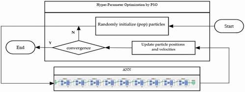
The flowchart of the proposed approach is displayed in Figure 2. The suggested technique used a number of particles (pop) which is initialized randomly. For each particle, the corresponding ANN is created and evaluated using a fitness function shown in equation (3)(3) $f_i=\frac{1}{m}\sum _1^m{\left(expectedoutpu{t}_i-actualoutpu{t}_i\right)}^2$(3) .

(3) $f_i=\frac{1}{m}\sum _1^m{\left(expectedoutpu{t}_i-actualoutpu{t}_i\right)}^2$(3)

Figure 2. The variation in the MSE vs. the population size.

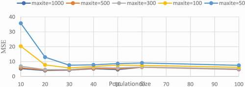
Figure 3. The relation between the number of iterations and the MSE.

Figure 4. Regression plot of the trained ANN using proposed technique.

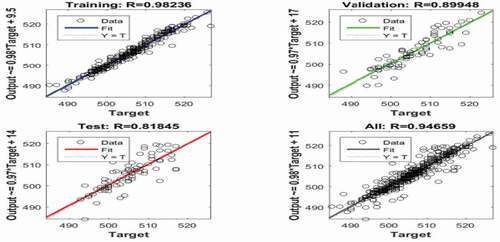
Figure 5. Mean Squared Error of the proposed technique using the train, validation,and test data.

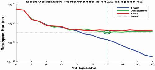
Figure 6. The relative error for all inputs in the dataset.

Figure 7. The comparison of the output of proposed technique with actual output and ANN output.

Figure 8. RE for proposed technique vs ANN without PSO.

where $m$ is the number of inputs for ANN.

The fitness values of all swarm are determined using equation (3)(3) $f_i=\frac{1}{m}\sum _1^m{\left(expectedoutpu{t}_i-actualoutpu{t}_i\right)}^2$(3) . The location and fitness value of each particle are stored as Xi and $Pbes{t}_i$ respectively. Among all pbest, the pbest with minimum fitness value is selected as the global best particle(gbest) and thus the location and fitness value of gbest are stored. This process is repeated by updating the particle positions and velocities according to equations (1)(1) $V_i^{\left(t+1\right)}=w.w.V_i^{\left(t\right)}+c_1{r}_1\left(P_i-X_i^{\left(t\right)}\right)+c_2{r}_2\left(P_g-X_i^{\left(t\right)}\right);i=1,2,\dots ,N$(1) and (2(2) $X_i^{\left(t+1\right)}=X_i^{\left(t\right)}+V_i^{\left(t+1\right)};i=1,2,\dots ,N,$(2) ). The process is iterated until the best solution is found or the maxite is reached. The global best particle represents the best selected hyper-parameters that used to build ANN.

Experimental Results and Performance Evaluation

In this section, the evaluation of the performance of the new technique is presented. The experimental dataset and settings of the experiment are described in detail. In addition, the experimental results of the proposed approach are discussed.

Dataset Description

In this subsection, the used datasets are described. To evaluate the suggested algorithm, the chemical sensor dataset was used. This dataset can be used to train a neural network to estimate one sensor signal from eight other sensor signals. The chemical dataset consists of an 8 ×498 matrix defining measurements taken from eight sensors during a chemical process used as inputs. In addition, the chemical dataset has a 1 ×498 matrix of a ninth sensor’s measurements, to be estimated from the first eight sensors and used as targets. This dataset was used to evaluate the proposed method using mean square error and regression analysis. In this paper, while 80% of the available data were used as a training set, 10% of the available data were used as a validation set, and the last 10% of the available data were used as a test set. The chemical sensor dataset can easily be loaded in MATLAB workspace by typing the following commands:

[input, target] =chemical-dataset;

inputs =input’;

targets =target’;

Settings of Experiment

To run the proposed method, the settings of PSO and multilayer neural network were set as follows: pop =20, maxite = 500, where pop is the swarm size while maxite is the maximum number of iterations. The values of c1, c2 were set to 2, and the values of Wmin, Wmax were set to 0.4 and 0.9, respectively (Sengupta, Basak, and Peters 2019), (Stang et al. 2020). We used a 2-dimensional search space (HL and NPHL) to represent the hyper-parameter of ANN. Initialization ranges for HL and NPHL were set to [1 7] and [14 21], respectively. The Levenberg-Marquardt (trainlm) function was used as the train function for the network. The Tansig function was used as an activation function of the networks.

Results and Discussion

In this subsection, the results of applying the proposed technique are presented and discussed. In addition, the proposed technique is compared with ANN without using PSO. To evaluate the performance of the suggested method, we modified the already existent MATLAB code of PSO and ANN packages according to our assumptions. To select the optimal configuration for the ANN, the proposed algorithm was tested in two different scenarios to determine the optimal settings for the proposed algorithm in terms of the population size and the number of iterations. In the first scenario, to show the effect of the population size on the proposed method, the population size was varied (pop = [10, 20, 30, 40, 50, 60,100]), while the maxite was kept constant for each population size. In the second scenario, the maximum number of iterations was varied (maxite = [25, 50, 100, 200, 300, 400, 500, 1000]), while the population size was kept constant at pop =20. The experiments were executed using a PC with Windows 8.1 operating system and Intel Core i5 processor running at 3.30 GHZ, 4 GB of RAM.

The result of the first scenario is presented in Figure 2. This Figure shows the variation in MSE against population size with the maxite equal to 1000, 500,300, 100, and 50. As can be seen from Figure 2, it is clear that the best population size with the minimum MSE is 20.

In the second scenario, to select the best maximum number of iterations the proposed technique was run for different values of iteration with a constant value for the population size (pop =20). Figure 3 displays the relationship between the number of iterations and MSE. It is clear that as the maximum number of iterations increases, the learning of the network increases, so as a result, the MSE decreases. It is also clear that the best number of iterations with the minimum MSE is 1000.

Table 1, displays the elapsed time (sec) according to the number of iterations.

Table 1. The elapsed time (sec)

Population Size (pop) = 20
Number of Iterations	Elapsed Time(sec)
25	17.86411
50	22.292923
100	31.592011
200	47.868706
300	64.288992
400	81.253257
500	110.071804
1000	175.033432

Now, to design the optimal architecture of the ANN, the proposed technique was run with the selected settings to determine the optimal hyper-parameters of the network in terms of the number of HL and NPHL. The result of running the proposed algorithm displays that the best configuration was selected by particle 10 with MSE equal to 3.9772%. The corresponding hyper-parameters, i.e., the number of HLs is equal to 2, and the number of NPHLs is equal to 15.

Although obtaining the optimal set of hyper-parameters of the ANN is a time-consuming process [26], the elapsed time to find the optimal configuration in the proposed technique was 175.033432 seconds. Thus, the proposed algorithm can be considered efficient in terms of processing time.

Furthermore, MSE is essential to measure the error between the predicted outputs of the network and the actual targets. The regression (R) value measures the correlation between the predicted outputs and targets. When R =1 that means a close relationship whereas R =0 indicates a random relationship between the outputs and targets. Plot regression used to validate the performance of the proposed technique; besides that, it provides an important analysis of the results. The regression plots show the expected outputs of the network with respect to actual targets for training, validation, and test sets. Figure 4 shows the regression plot of the trained ANN with the selected hyper-parameters using the proposed algorithm. The regression coefficient R for training, validation, test, and all are 0.98236, 0.89948, 0.81845, and 0.94659, respectively. In addition, as can be seen the fit line for data fall along a 45-degree line approximately, which means that the network outputs are almost equal to the targets. Thus, the accuracy of the proposed method can be considered as excellent.

The best validation performance plot against the number of training epochs is shown in Figure 5. As can be seen the best value of validation performance is 11.22 at epoch

12, while the training is continued for six more iterations before it stopped. The best MSE value of training is 0.03977.

As can be seen, the performance curve starts with a high value of MSE (equal to 3124.429). This is because, at the start running of the technique, the values of hyper-parameters were initiated randomly which may not be suitable. Therefore, the differences between the expected outputs and targets for 498 items in the used dataset were big and as a result the initial value of MSE was very big. However, after training the network using the proposed technique frequently, the error decreased and thus MSE decreased. Generally, the error was reduced after more epochs of training. In the proposed technique the MSE value reached 0.03977, indicating the efficiency of applying the proposed technique. Now, the trained neural network called “net_final_selected” can be applied to predict the output of input features. Let the input feature for the net_final_selected of the mentioned dataset is tested_input which is given as tested_input = [152, 9739, 4895, 380, 2.78, 408, 565, 447508]; and the actual corresponding target is 515. To predict the corresponding output for this input using the trained ANN, the following MATLAB code is needed to be written: expected_output = net_final_selected (tested_input ‘).; This produces the following output as can be seen.

>> tested_input= [152, 9739, 4895, 380, 2.78, 408, 565, 447508];

>> expected_output=net_final_selected (tested_input’)

expected_output =

As can be seen the trained network using the proposed technique is giving the expected output with a relative error equal to 0.3%. This relative error for $inpu{t}_i$in the dataset can be calculated as follows:

$erro{r}_i=(net\mathrm{\_}final\mathrm{\_}selected(inpu{t}_i)-targe{t}_i)/targe{t}_i$ (3),(4)

This result demonstrates that the proposed algorithm has very high accuracy. Figure 6 shows the relative error for all the inputs in the dataset. As can be seen, the error value ranges from 0% to 1.6%.

Finally, to study the efficiency of the proposed technique, a comparison of this technique with the ANN without using PSO was carried out. Figure 7 shows the comparison between the expected output of the proposed technique, the expected output of ANN without using PSO, and the actual output. In this In this comparison, the output was computed using random samples of the input’s values from the dataset.

As can be seen from Figure 7, it is clear that the convergence of the expected output of the proposed technique to the actual output with a very small error is better compared with the expected output of the ANN without using PSO. Consequently, the proposed technique achieves higher accuracy than the ANN. The relative error (RE) is calculated using some random samples of the input values. RE for both the proposed technique and ANN without using PSO is shown in Figure 8.

As shown in Figure 8, RE of the proposed technique is significantly lower than RE of the ANN. Therefore, the quality of the solutions provided by the proposed technique is higher than that provided by ANN.

Conclusion and Future Work

In this paper, a new technique is presented to select the optimal configuration for the multilayer ANN using PSO. The proposed method is tested using a chemical dataset to evaluate the effectiveness of our method. The results show that the proposed technique is able to select the optimal hyper-parameters used to construct the desired network with very high accuracy of prediction with a percentage error of no more than 3.9%. Moreover, the proposed technique displayed better performance compared with ANN in terms of the accuracy of the prediction.

For future work, we suggest the study of the effect of changing NPHL for each layer instead of being the same in all hidden layers in the proposed algorithm. We also suggest extending the proposed approach to discuss the ability of selecting more hyper-parameters such as the activation function, the number of iterations, the learning rate, and the size of a batch. In addition, future work may discuss the effect of the activation function if we apply the same activation function for all the layers or if we apply different activation function for each layer. Moreover, applying an improved PSO to train the NN and compare its results with the proposed algorithm is a worthy work. Furthermore, a comparison of the proposed technique with other techniques such as GA, or ACO can be carried out. Finally, the proposed method can be applied against different datasets such as the oil reservoir dataset or COVID-19 dataset.

References

- Ananthi, J., and V. Ranganathan. 2016. Multilayer perceptron weight optimization using Bee swarm algorithm for mobility prediction. IIOAB Journal 7 (9):47–63.
- Bacanin, N., T. Bezdan, E. Tuba, I. Strumberger, and M. (v) Tuba. 2020. Optimizing convolutional neural network hyperparameters by enhanced swarm intelligence metaheuristics. Algorithms 13 (3):67. doi:https://doi.org/10.3390/a13030067.
- Devyani, B., and S. Poonam. 2018. Review on reliable pattern recognition with machine learning techniques. Fuzzy Information and Engineering 10 (3):362–77. doi:https://doi.org/10.1080/16168658.2019.1611030.
- Frazier, M., C. Longo, B. S. Halpern, and S. J. Bograd. 2016. Mapping uncertainty due to missing data in the global ocean health index. PLoS ONE 11 (8):e0160377. doi:https://doi.org/10.1371/journal.pone.0160377.
- Ghanou, Y., and G. Bencheikh. 2016. Architecture optimization and training for the multilayer perceptron using ant system. International Journal of Computer Science 43 (1):10.
- Guoqiang, P. Z. 2000. Neural networks for classification: A survey. IEEE Transactions on Systems, Man, and Cybernetics 30 (4):451–62. doi:https://doi.org/10.1109/5326.897072.
- Hecht-Nielsen, R. 1988. Theory of the backpropagation neural network. Neural Networks 1 (Supplement–1):445–48. doi:https://doi.org/10.1016/0893-6080(88)90469-8.
- Islam, B. U., Z. Baharudin, M. Q. Raza, and P. Nallagownden. 2014. Optimization of neural network architecture using genetic algorithm for load forecasting. In: 2014 5th International Conference on Intelligent and Advanced Systems (ICIAS), Kuala Lumpur, Malaysia, p. 1–6
- Jamous, R., A. Tharwat, E. El. Seidy, and B. Bayoumi. 2015. A new particle swarm with center of mass optimization. INTERNATIONAL JOURNAL OF ENGINEERING RESEARCH & TECHNOLOGY (IJERT) 04 5 (May), 312-317.
- Jiansheng, W., O. JinL, and L. Mingzhe. January 19 2015. Evolving RBF neural networks for rainfall prediction using hybrid particle swarm optimization and genetic algorithm. In Neurocomputing Journal 148: 136–42. doi:https://doi.org/10.1016/j.neucom.2012.10.043.
- Mustafa, A. S., and Y. S. K. Swamy. 2015. Web service classification using multi-layer perceptron optimized with Tabu search. In: Advance Computing Conference (IACC), 2015 IEEE International, Banglore, India, p. 290–94.
- Oludare, A., J. Aman, O. Abiodun, D. Kemi, M. Nachaat, and A. Humaira. 2018. State-of-the-art in artificial neural networkapplications: A survey. Heliyon.4 (11): e00938.
- Qolomany, B., M. Maabreh, A. Al-Fuqaha, A. Gupta, and D. Benhaddou 2017. Parameters optimization of deep learning models using particle swarm optimization, 13th International Wireless Communications and Mobile Computing Conference (IWCMC), Valencia, 2017, Valencia, Spain, pp. 1285–90.
- Sengupta, S., S. Basak, and R. A. Peters. 2019. Particle swarm optimization: A survey of historical and recent developments with hybridization perspectives. Machine Learning and Knowledge Extraction 1 (1):157–91. doi:https://doi.org/10.3390/make1010010.
- Shi, Y., and R. Eberhart. 1999. Empirical study of particle swarm optimization. International Conference on Evolutionary. Washington, USA: Computation.
- Sohrab Z., M. A., L. Ali, E. Ali, and C. Ioannis. 2012. Reservoir permeability prediction by neural networks combined with hybrid genetic algorithm and particle swarm optimization. Geophysical Prospecting 61 (3):582-598.
- Stang, M., C. Meier, V. Rau, and E. Sax. 2020. An evolutionary approach to hyper-parameter optimization of neural networks. In Human interaction and emerging technologies. IHIET 2019. Advances in intelligent systems and computing, vol 1018, ed. T. Ahram, R. Taiar, S. Colson, and A. Choplin. pp. 713-718. Cham: Springer.
- Xin, J., G. Chen, and Y. Hai. 2009. A particle swarm optimizer with multi-stage linearly-decreasing inertia weight. International Joint Conference on Computational Sciences and Optimization, Sanya, Hainan, pp. 505–08, doi: https://doi.org/10.1109/CSO.420.
- Xu, D., and Y. A. Tian. 2015. Comprehensive survey of clustering algorithms. Annals of Data Science 2 (2):165–93. doi:https://doi.org/10.1007/s40745-015-0040-1.
- Xu, Z., Zhang, J., Wang, J., and Xu Zh. 2020. Prediction research of financial time series based on deep learning. Soft Computing. 24(11):8295–312. doi:https://doi.org/10.1007/s00500-020-04788-w.
- Yamasaki, T., T. Honma, and K. Aizawa. 2017. Efficient optimization of convolutional neural networks using particle swarm optimization. in: IEEE Third International Conference on Multimedia Big Data, Laguna Hills, CA, USA, pp. 70–73.
- Ye, F., and W.-B. Du. 2017. Particle swarm optimization based automatic parameter selection for deep neural networks and its applications in large-scale and high-dimensional data. PLoS ONE 12 (12):e0188746. doi:https://doi.org/10.1371/journal.pone.0188746.
- Yulong, W., Z. Haoxin, and Z. Guangwei. 2019. cPSO-CNN: An efficient PSO-based algorithm for fine-tuning hyper-parameters of convolutional neural networks. Swarm and Evolutionary Computation 49:114–23. doi:https://doi.org/10.1016/j.swevo.2019.06.002.
- Zajmi, L., H. A. Falah, and A. J. Adam. 2018. Concepts, methods, and performances of particle swarm optimization, backpropagation, and neural networks. Applied Computational Intelligence and Soft Computing vol:1–7. doi:https://doi.org/10.1155/2018/9547212.