A Recurrence Population-based Great Deluge Algorithm with Independent Quality Estimation for Feature Selection from Academician Data

ABSTRACT

Great deluge (GD) algorithm same as other metaheuristics can solve feature selection problem. The GD imitates that in a great deluge someone climbing a hill and attempt to progress in any direction that does not get his/her feet wet in the expectation of discovering a way up when the water Level rises. The drawbacks of GD are: 1) a local search, which may lead the algorithm toward a local optima and 2) a challenging estimation of quality of the final solution in solving most of the problems. In this paper, for the first issue, a population-based great deluge (popGD) algorithm with additional recurrence operation is proposed. This operation is an imitation of no progress of hill climber after a long time; the climber tries to move small steps even downward in hope of finding better way to climb. For the second problem, a technique with an automate alteration of the Level is proposed. The statistical analysis of the results from 25 test functions and 18 benchmark feature selection problems supports the ability of the method. Finally a real-world academician data are employed to perform feature selection and execute classification result with selected features.

Introduction

Feature selection is considered as an important and necessary step (pre-processing) before performing any data mining task and data engineering. Selection of a subset of the full feature set while still describes the original and full feature set with less information loss is defined as feature selection (Han, Kamber, and Pei 2011). Rough set theory presented in (Pawlak 1982) as a filter-based tool determines the relations between conditional features and decision feature. Rough set feature selection is performed by only using the data and no extra information.

Searching for a minimal subset of original feature set with the same level of discernibility of all features using metaheuristic algorithms is a common method in literature. See for example (Abdullah and Jaddi 2010; Aljarah et al. 2018; Derrac et al. 2012; Jaddi and Abdullah 2013c, 2013a, 2013b; Liang et al. 2014; Mafarja, Abdullah, and Jaddi 2015; Mafarja et al. 2018; Mafarja and Mirjalili 2018, 2017; Zeng et al. 2015). Simulated annealing was used to solve feature selection in many researches such as practices in (Lin et al. 2008; Meiri and Zahavi 2006). Tabu search was also applied to feature selection problem in (Tahir, Bouridane, and Kurugollu 2007; Zhang and Sun 2002). A greedy heuristics have been applied for rough set feature selection in (Zhong, Dong, and Ohsuga 2001). A multivariate feature selection approach has been solved using a random sub-space method in (Lai, Marcel, and Wessels 2006). Memetic algorithm was also proposed in (Zhu, Ong, and Dash 2007) for feature selection. Different versions of ant colony optimization (ACO) were presented in (Chen, Miao, and Wang 2010) and (Kabir, Shahjahan, and Murase 2012) for the same problem. A selection of gene expression data was practiced in (Abusamra 2013). A version of particle swarm optimization (PSO) approach using decision tree was presented in (Zhang et al. 2014) for selection of features. In (Rodrigues et al. 2014), same problem was solved using a bat algorithm (BA). Fuzzy population-based algorithm was also used for feature selection in (Mafarja, Abdullah, and Jaddi 2015). Another research (Emary, Zawbaa, and Hassanien 2016) shows the ability of binary ant line optimization (ALO) algorithm for feature selection. Electromagnetic-like algorithm also solved this problem in (Abdolrazzagh-Nezhad and Izadpanah 2016). Two versions of whale optimization-based algorithms (WOA) were presented in (Mafarja and Mirjalili 2017) and (Mafarja and Mirjalili 2018) to solve feature selection problem. Binary butterfly optimization approaches for feature selection was proposed in (Arora and Anand 2019). Feature selection strategy based on hybrid crow search optimization algorithm integrated with chaos theory and fuzzy c-means algorithm for medical diagnosis was presented in (Anter and Ali 2020). In another research presented in (Tubishat et al. 2019), an improved whale optimization algorithm for feature selection in Arabic sentiment analysis was proposed. A filter-based bare-bone particle swarm optimization algorithm for unsupervised feature selection was studied in (Zhang et al. 2019). A hybrid nature-inspired binary optimizers for feature selection was proposed in (Mafarja et al. 2020). A Research on feature selection for rotating machinery based on Supervision Kernel Entropy Component Analysis with Whale Optimization Algorithm was performed in (Bai et al. 2020).

Great deluge algorithm (GD) (Dueck 1993) (Figure 1), which is a single-solution, in many features is similar to hill climbing (HC) and simulated annealing (SA) algorithms. The name of GD comes from the similarity that in a great deluge someone does hill climbing and attempt to track any direction. In this climbing the person tries to not get his/her feet wet expecting to find a way up while the water level is increased. In original GD a single solution represents the position of person and the new solution is calculated to find a new position of the person. The value of level represents the water level and is increased in each iteration based on the quality of current solutions and also estimated quality of the final solution. The acceptance of the current solution depends on value of level in the current iteration. GD has been employed to solve many problems in literature such as researches in (Acan and Ahmet 2020; Baykasoglu 2012; Baykasoglu, Durmusoglu, and Kaplanoglu 2011; McCollum et al. 2009; Mcmullan 2007; Mosbah and Dao 2010; Nahas et al. 2008; Nourelfath, Nahas, and Montreuil 2007).

Figure 1. Pseudocode of GD algorithm

In this paper, new version of GD is proposed in which surmounts the two weaknesses of GD. The weaknesses are: 1) Getting stuck in local optima due to searching around single solution same as other single-solution heuristics. 2) Challenging estimation of quality of final solution for most of the problems. In order to solve the first problem, a population of single solutions is generated and each single solution follows the local search around itself and tries to improve the quality of solution in each iteration. This increases the exploration of the algorithm. In addition to this modification, all single solutions in population use a new operation called recurrence operation. This operation provides possibility of jumping from local optima. The recurrence operation is simulation of when a hill climber stuck during the climbing and no progress after a long time; the climber makes small moves around even downward in hope of finding better way to climb. These two modifications offer better exploration and reduce the risk of getting stuck in local optima (first drawback). To overcome the second drawback, an automate alteration of the Level is proposed in which eliminates the need for estimation of quality of final solution.

The proposed algorithm is tested using 25 test functions, and the results are compared and analyzed using statistical analysis. Furthermore, 18 benchmark feature selection problems are used to investigate the performance of the proposed method when it is applied for feature selection. The statistical analysis and the box plot graphs support the ability of the method. In addition, the method is applied to real-world academician publication data for feature selection and classification accuracy of the selected features is computed.

The rest of this paper is organized as follows: Section 2 provides a brief explanation of the basic GD algorithm as preliminary subject. The details of the proposed method are given in section 3. Discussion and analysis of the experimental results when the algorithm is applied on benchmark test functions, benchmark feature selection and real-world feature selection problems in section 4. The work is concluded in Section 5 in this paper.

The GD Algorithm

The GD algorithm firstly proposed in (Dueck 1993) as a local search metaheuristic algorithm. This algorithm accepts the solutions that improve the quality of the best solution found so far. The worse solutions are also accepted in this algorithm if the quality of these solutions is better than boundary level with hopes of improving the quality of the best solution. In initialization part of this algorithm, the level is set to quality of initial solution. The value of level is increased or decreased (depends on minimization or maximization approaches) using a fixed rate β during the search process. The value of β is calculated based on the quality of initial solution and estimated quality of the final solution as is shown in Eq. (1)(1) $\beta =(EQ-f_{(sol)})/iterationNum$(1) :

(1) $\beta =(EQ-f_{(sol)})/iterationNum$(1)

In this equation, the EQ is estimated quality of the final solution, f_(sol) is quality of initial solution and the iterationNum is predefined number of iterations.

set initial solution, Sol

set best solution, Sol_best

set current solution, Sol_current

set initial level, Level

set iteration ← 0

set number of iterations, iterationNum

calculate the value of β by Eq. 1(1) $\beta =(EQ-f_{(sol)})/iterationNum$(1)

do while (iteration < iterationNum)

create new solution, Sol_new

evaluate Sol_new

if Sol_new is better than Sol_best

update Sol_current and Sol_best

else

if Sol_new better than Level

update Sol_current

endif

endif

update the Level

increase iteration

end while

return Sol_best

This algorithm starts with a single solution and tries to find a better solution around it. In each iteration, the current solution and the best solution are updated based on the quality of the current solution. If the quality is better than the best solution found so far, the best solution is updated. Otherwise, if the quality is better than the value of level in the current iteration, the current solution is only updated. Accepting the worse solution as current solution in this algorithm keeps the region of the search slightly wider when we compare it with hill climbing algorithm. From the other side, the boundary level used in this algorithm provides more focus of the algorithm on better solutions.

Proposed Method

Three major modifications are applied on basic GD to improve the performance of the algorithm. The first modification is to use the advantages of the population of this algorithm. The second modification is the application of recurrent operation and the third amendment is to avoid the estimation of quality of the final solution.

A population of random candidate solutions is generated in first step of algorithm. The quality of the solutions is calculated. The best solution within all is found. The value of the Level is initialized. Each solution works as a single-solution GD in which each one generates a new solution. If the new solution in neighborhood of current solution is better than the best the best solution is updated, otherwise, if the new solution is better than the value of level this solution is accepted as current solution. The recurrence operation is performed if after a certain number of iteration there is no improvement in quality of the best solution. All solutions in population follow the same process with the same value of the Level. After visiting of all solutions in population the value of Level is automatically altered by calculation the value of β where there is no need to estimation of quality of final solution. The next iteration is started in this stage. The repetition of this process is performed until termination criterion is reached.

The recurrence operation is performed if after a defined number of iterations, improvement of the quality in best solution is not observed. A number of solutions in neighborhood of the current solution are generated and the best among them is selected to be as candidate solution. This is an extension of GD which is simulation that a hill climber ties to go up in any direction that his/her feet does not get wet in great deluge. The recurrence operation is a simulation of when the hill climber gets stuck somewhere during the hill climbing and progress is difficult to perform. The climber decides to move around to find a way easier for progress.

The value of Level in increased during the search process and the rate of incrimination is calculated using the value of β. In basic GD, this value is constant which presents a linear boundary of Level. In popGD, a nonlinear boundary Level with independent estimation of the final quality is used. This provides a boundary Level which is effective with no challenging process of estimation. Furthermore, it reduces the number of parameters for the algorithm. The GD with modifications is shown in the flowchart and pseudocode in Figure 2 and Figure 3, respectively.

set initial population

set number of solutions in population, popSize

set i^th solution in the population, Sol_i

set best solution around sol_i, best_i

set current solution around sol_i. current_i

set best solution among all in population, Sol_best

set initial level, Level

set β← 0

set iteration ← 0

set i ← 0

set number of iterations, iterationNum

do while (iteration < iterationNum)

for all solutions (Sol_i) in population

evaluate Sol_i

if Sol_i better than best_i

update current_i and best_i

else

if Sol_i better than Level

update current_i

endif

endif

if there is no improvement after certain number of iteration

apply recurrence operation

endif

update the Sol_best

endfor

update Sol_best

calculate the β and update the Level

increase iteration

endwhile

return Sol_best

Figure 2. Flowchart of popGD

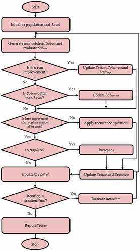
Figure 3. Pseudocode of popGD

Based on modifications applied on GD algorithm, the algorithm can search more globally with no estimation of quality of final solution using a nonlinear level. The details of the modifications are explained in following subsections.

Population for Great Deluge

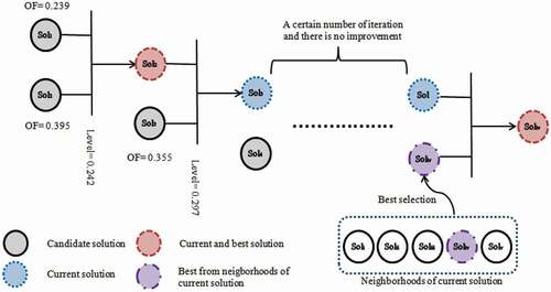
The GD algorithm is a local search approach, and it searches a region of the search space that initial solution is located. Therefore, quality of final solution depends on location of initial solution. In local search algorithms the possibility of getting stuck in local optimum is high for the same reason. Since population-based algorithms, explore the search space globally, the popGD similar to other population-based algorithms uses a population of solutions. In popGD, a population of single solutions walks around the search space while each one search locally around itself and tries to improve its quality. In this algorithm, each single solution works separately but in parallel with other solutions. This process is similar to a competition between the solutions. The effort of each solution is to find a better solution in its neighborhoods. In popGD, each solution in the population follows the same process as other solutions in population. The solution better than the best solution within the neighborhoods, is updated as best solution of this region. The worse solutions are also accepted as the current solution if they are better than the level. The value of level is equal for all solutions in the population in each iteration. The overall process of population activities is shown in Figure 4.

Figure 4. Schematic example of population activity in popGD

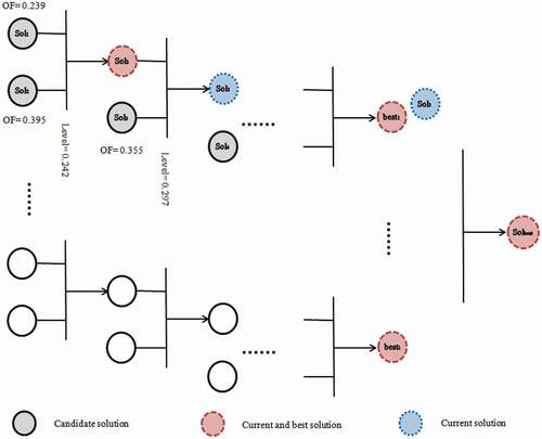
In this figure, the objective function (quality of the solution) is shown by OF. This figure shows each solution in population searches its neighborhoods separately in parallel and the best solution found by each solution is compared with the overall best solution and is updated. This process enhances the exploration ability of the algorithm.

Recurrence Operation

As it is mentioned before, there is possibility for the GD, as a local search algorithm that gets stuck in local optima. Using a population of solutions and working in different regions of the search space (first modification of GD presented in previous section) provides searching the whole regions of the search space and decrease the risk of getting stuck in local optima. In addition to this, modification and to improve this maintenance, a recurrence operation is proposed in popGD.

As it is mentioned before, the GD is the imitation of how a hill climber performs progress upwards in great deluge. The recurrence operation, as an enhancement of GD, is an imitation that the hill climber gets stuck in hill somewhere for a long time and it seems that no more progress is possible. In this time the climber decides that make a small move around even downward to find a better way to climb. In popGD, during the search process using population of single solutions in different part of search space, if after a defined number of iterations, the improvement in quality of the best solution is not observed, the recurrent operation is applied on the current solution. Recurrent operation is generation of different solutions in neighborhood of current solution and selection of the best with better quality among them and using the selected solution as current candidate solution with hope of finding a better solution compared to the best so far. This provides the possibility of the jumping from the local area and increase the opportunity of searching the search space globally. The schematic example of recurrence operation in popGD is presented in Figure 5.

Figure 5. Schematic example of recurrence operation in popGD

Rate of Altering the Value of Level

Another modification to basic GD is to enhance the calculation of value of β. In basic GD, the value of β is a fixed value, which is calculated based on the quality of the initial candidate solution, the estimated quality of the final solution and the predefined number of iterations. The calculation of the value of β is performed (Eq. 1)(1) $\beta =(EQ-f_{(sol)})/iterationNum$(1) only once in the initialization part of the algorithm and the same value is used to update the level with linear manner in each iteration. There are two drawbacks of using this calculation (Eq. 1)(1) $\beta =(EQ-f_{(sol)})/iterationNum$(1) of the value of β. Firstly the estimated quality of the final solution is slightly difficult in solving most of the problems. This may be a challenge to estimate the quality of the final solution for researchers. The second drawback is that the fixed value of β provides the algorithm with a linear boundary level, which may not really effect on finding optimum solutions. To surmount the drawbacks Eq. 2(2) $\beta =\frac{iteration}{iterationNum\times f_{(So{l}_{best})}}$(2) is proposed.

(2) $\beta =\frac{iteration}{iterationNum\times f_{(So{l}_{best})}}$(2)

In this equation iteration is the current iteration, iterationNum is the predefined number of iterations and f_(Solbest) is quality of the best solution found so far. This equation is calculated in each iteration automatically and as it is clear in this equation, it is affected from quality of best solution so far. This provides the nonlinearity of the value of β and subsequently the value of Level during the search process.

Experimental Results

In this section, results of application of the proposed method on both benchmark problems and real-world problem is presented and discussed.

Experimental Results for Benchmark Problems

This sub-section provides the results of two experiments. Firstly, the basic GD and the popGD are applied on 25 CEC 2005 benchmark test functions, and the results are compared and analyzed. In the second experiment, the results of GD and popGD are applied on 18 benchmark classification data for feature selection. The results of feature selection are used for classification and the accuracy of classification of the results are compared and analyzed. The statistical analysis is used to evaluate the performance of the popGD in both experiments.

i. Results for Test Functions

In this experiment, 25 test functions (CEC 2005 benchmark functions) were tested to assess the performance of the popGD. Table 1 presents the details of the tested functions. The details in this table are: the key for the function, the name of each function, the variables value range, the category of each function, and the optimal value f(x). The unimodal (U), multimodal (M), shifted (S1), separable (S2), scalable (S3), non-separable (N), and rotated (R) are a category of CEC 2005 benchmark functions.

Table 1. Details of the CEC 2005 test functions

Key	Test function	Range	Category	f(x)
f1	Shifted Sphere Function	[−100,100]	US1S2S3	−450
f2	Shifted Schwefels Problem 1.2	[−100,100]	UNS1S3	−450
f3	Shifted Rotated High Conditioned Elliptic Function	[−100,100]	URNS1S3	−450
f4	Shifted Schwefels Problem 1.2 with Noise in Fitness	[−100,100]	UNS1S3	−450
f5	Schwefels Problem 2.6 with Global Optimum on Bounds	[−100,100]	UNS3	−310
f6	Shifted Rosenbrocks Function	[−100,100]	MNS1S3	390
f7	Shifted Rotated Griewanks Function without Bounds	[0,600]	URNS1S3	−180
f8	Shifted Rotated Ackleys Function with Global Optimum on Bounds	[−32,32]	URNS1S3	−140
f9	Shifted Rastrigins Function	[−5,5]	MS1S2S3	−330
f10	Shifted Rotated Rastrigins Function	[−5,5]	MRNS1S3	−330
f11	Shifted Rotated Weierstrass Function	[−0.5,0.5]	MRNS1S3	90
f12	Schwefels Problem 2.13	[-π,π]	MNS1S3	−460
f13	Expanded Extended Griewanks plus Rosenbrocks Function (F8F2)	[−5,5]	MNS1S3	−130
f14	Shifted Rotated Expanded Scaffers F6	[−100,100]	MNS1S3	−300
f15	Hybrid Composition Function	[−5,5]	MS2S3	120
f16	Rotated Hybrid Composition Function	[−5,5]	MRNS3	120
f17	Rotated Hybrid Composition Function with Noise in Fitness	[−5,5]	MRNS3	120
f18	Rotated Hybrid Composition Function	[−5,5]	MRNS3	10
f19	Rotated Hybrid Composition Function with a Narrow Basin for the Global Optimum	[−5,5]	MNS3	10
f20	Rotated Hybrid Composition Function with the Global Optimum on the Bounds	[−5,5]	MNS3	10
f21	Rotated Hybrid Composition Function	[−5,5]	MRNS3	360
f22	Rotated Hybrid Composition Function with High Condition Number Matrix	[−5,5]	MNS3	360
f23	Non-Continuous Rotated Hybrid Composition Function	[−5,5]	MNS3	360
f24	Rotated Hybrid Composition Function	[−5,5]	MRNS3	260
f25	Rotated Hybrid Composition Function without Bounds	[2,5]	MRNS3	260

The methods compared in this experiment were run 100 times for each test function presented in Table 1. In order to compare the results the mean of 100 results and the standard deviation (Std. Dev.) of the results were calculated and are presented in Table 2. For the comparison purpose, the mean of 100 runs of each algorithm for each test function reported in Table 2 can be compared with optimum solution given in Table 1. Note that all test functions used in this experiment are minimization problems. Table 2 shows superior results of popGD compared to GD. This higher ability of popGD is due to searching the search space globally and more exploration during the search process. This ability is provided using a population of the solutions and exploring the search space by a parallel procedure of GD. This process affects searching different regions of the search space with the aim of looking for the optimum solution globally. Recurrence operation, which possibly avoids getting stuck in local optima is another reason for effectiveness of the method.

Table 2. Comparison of the results for the CEC 2005 test functions

Test function	GD		popGD
	Mean	Std. Dev.	Mean	Std. Dev.
f1	−437.5431	5.9377	−441.7040	7.5440
f2	−439.1867	7.0296	−444.5747	7.4196
f3	−444.4195	7.3026	−446.8994	5.5925
f4	−443.6752	7.1820	−444.9597	6.8012
f5	−307.8300	2.7149	−308.5443	2.8878
f6	386.9645	2.2920	388.8551	2.5652
f7	−179.2069	0.6198	−179.7931	0.4122
f8	−138.1030	1.0122	−139.0340	0.7784
f9	−329.2070	0.4122	−329.6210	0.4938
f10	−329.3790	0.4938	−329.7240	0.4548
f11	90.4827	0.5085	90.2413	0.4354
f12	−459.5860	0.5012	−459.8970	0.3099
f13	−129.6550	0.4837	−129.8970	0.3099
f14	−298.6510	0.8272	−298.9610	0.6128
f15	120.9310	0.9975	120.1379	0.3509
f16	120.1034	0.3099	120.1379	0.3509
f17	121.6915	0.7991	120.9818	1.0253
f18	10.7586	0.7862	10.3793	0.6218
f19	11.1724	0.7105	10.5172	0.8709
f20	10.9310	0.7987	10.5172	0.7847
f21	361.0172	0.5258	360.4138	0.6822
f22	360.8793	0.5924	360.3103	0.4708
f23	360.6897	0.6996	360.2586	0.2542
f24	260.7931	0.4122	260.3448	0.4837
f25	260.4483	0.5061	260.2069	0.4122

A t-test analysis was carried out and the p-value results were computed to make a more detailed comparison. The results of this analysis are shown in Table 3. The critical value α is equal to 0.05 in this statistical analysis. The values lower than α indicate that there is a significant difference between the results of GD and popGD. The values lower than 0.05 (critical value) are presented in bold in Table 3.

Table 3. Pairwise comparison of GD and popGD for the CEC 2005 test functions

Test function	P-value	Test function	P-value
f1	0.0225	f14	0.0457
f2	0.0021	f15	7.76E-05
f3	0.1043	f16	0.3313
f4	0.2468	f17	0.0004
f5	0.0006	f18	0.0308
f6	0.0057	f19	0.0014
f7	0.0001	f20	0.0381
f8	0.0001	f21	0.0005
f9	0.0006	f22	0.0001
f10	0.0077	f23	0.0028
f11	0.0251	f24	0.0007
f12	0.0086	f25	0.0349
f13	0.0160	-	-

ii. Results for Feature Selection

The popGD algorithm proposed in this paper was applied to UCI classification datasets (Blake and Merz 1998) in order to do feature selection and later use the selected features for solving classification problem. The details of 18 UCI datasets examined in this experiment are presented in Table 4.

Table 4. List of datasets employed for feature selection

Dataset	No. of features	No. of objects
Breastcancer	9	699
BreastEW	30	569
CongressEW	16	435
Exactly	13	1000
Exactly2	13	1000
HeartEW	13	270
IonosphereEW	34	351
KrvskpEW	36	3196
Lymphography	18	148
M-of-n	13	1000
PenglungEW	325	73
SonarEW	60	208
SpectEW	22	267
Tic-tac-toe	9	958
Vote	16	300
WaveformEW	40	5000
WineEW	13	178
Zoo	16	101

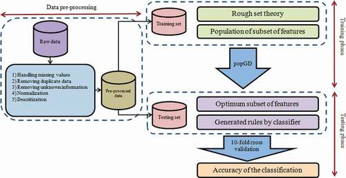
Pre-processing techniques such as handling missing values, removing noise and discretization were carried out to the raw data in order to make the data applicable to the model. In this experiment one-dimensional vector with N cells, where N was the number of features in the full feature set is used for each solution representation. Each cell held one element. Each element was assigned a value of ‘1ʹ or ‘0ʹ, where ‘1ʹ denoted the selection of the corresponding feature, otherwise ‘0ʹ.

As we applied the rough set approach for solving feature selection problem, a subset of the full feature set with a highest dependency degree (preferably equal to 1) and lowest number of features was searched. The fitness function used in this experiment is calculated based on dependency degree and a number of features and is shown in Eq. (3)(3) $F(R)={\gamma }_R(D)\ast \frac{\left|C\right|-\left|R\right|}{\left|C\right|}$(3) :

(3) $F(R)={\gamma }_R(D)\ast \frac{\left|C\right|-\left|R\right|}{\left|C\right|}$(3)

In this equation R represents a subset of the full feature set and C is the conditional feature set. The decision feature is shown by D and γ_R (D) dependency degree of D.

The overall process of this experiment is shown in Figure 6. The algorithm was run 20 times in this experiment and the selection ratios (number of selected features/number of features in the full feature set) was calculated for each dataset. The average and standard deviations (Std. Dev.) of 20 ratios are shown in Table 5.

Table 5. Comparison of average selection ratio between GD and popGD

	GD		popGD
Test function	Mean	Std. Dev.	Mean	Std. Dev.
Breastcancer	0.6012	0.0804	0.4710	0.0439
BreastEW	0.6300	0.0415	0.5196	0.1521
CongressEW	0.6280	0.0665	0.5852	0.1552
Exactly	0.6106	0.0411	0.6222	0.1553
Exactly2	0.5026	0.0592	0.4146	0.1294
HeartEW	0.6493	0.0267	0.5283	0.1357
IonosphereEW	0.5879	0.0697	0.4119	0.1197
KrvskpEW	0.7285	0.0119	0.6798	0.1858
Lymphography	0.4757	0.0161	0.4481	0.1352
M-of-n	0.7082	0.0555	0.4633	0.1246
PenglungEW	0.3656	0.0382	0.3378	0.0910
SonarEW	0.7542	0.0271	0.6931	0.2050
SpectEW	0.4816	0.0680	0.3573	0.1447
Tic-tac-toe	0.7531	0.0298	0.7031	0.2032
Vote	0.4546	0.0239	0.3407	0.1376
WaveformEW	0.8050	0.0250	0.7892	0.2300
WineEW	0.6476	0.0415	0.6062	0.1524
Zoo	0.6604	0.0257	0.6241	0.1534

Figure 6. Overall process of feature selection and classification

The comparison of average selection ratio for the popGD and GD in Table 5 shows lower average selection ratio for popGD in most of the datasets in this experiment. In order to statistical analysis and comparison, a t-test analysis was performed and the p-value results computed are shown in Table 6. The value of critical level for this experiment was equal to 0.05 same as in the t-test carried out for the test functions (in the previous sub-section). In Table 6, the values less than the value α show a major difference between the results of the popGD and the GD. The values lower than α are presented in bold in Table 6. The superiority of popGD is clearly being shown when is compared to the GD in this table. The results show that using population of single solutions in GD algorithm results a better exploration and leads the algorithm toward a superior solution. This is the reason for superior ability of the results of popGD compared to GD.

Table 6. Pairwise comparison of popGD and GD for feature selection

Dataset	p-value	Dataset	p-value
Breastcancer	2.66E-06	M-of-n	9.94E-12
BreastEW	6.39E-06	PenglungEW	0.0220
CongressEW	0.0381	SonarEW	0.0004
Exactly	0.2343	SpectEW	7.09E-07
Exactly2	0.0004	Tic-tac-toe	0.0027
HeartEW	3.58E-09	Vote	6.77E-11
IonosphereEW	4.01E-10	WaveformEW	0.0371
KrvskpEW	2.18E-05	WineEW	0.0025
Lymphography	0.0014	Zoo	3.67E-06

The Rosetta software was used to generate the rules from selected features found by GD and popGD and then the generated rules were used to classify the datasets using standard voting classifier. This process was performed for the best result of feature selection within 20 runs for all datasets. The results of classification accuracy for the GD and popGD are shown and compared in Table 7. To predict the classification accuracy the 10-fold cross-validation was performed and the dataset was divided into two parts. The 70% of the data was used in the training set and the rest 30% was used for the testing set. Better classification accuracy of popGD reported in Table 7 using fewer features selected by popGD (as is shown in Table 6) proofs the ability of popGD which uses the advantage of having population with additional recurrence operation to explore the search space.

Table 7. Results for classification accuracy using selected features by the GD and popGD

Dataset	GD	Std. Dev.	popGD	Std. Dev.
Breastcancer	0.8916	0.0267	0.9510	0.0258
BreastEW	0.8970	0.0304	0.9741	0.1913
CongressEW	0.9206	0.0159	0.9617	0.1609
Exactly	0.8237	0.0145	0.9271	0.1556
Exactly2	0.7167	0.0086	0.7488	0.1371
HeartEW	0.7839	0.0096	0.8043	0.1334
IonosphereEW	0.8884	0.0054	0.9295	0.1655
KrvskpEW	0.9027	0.0299	0.9517	0.1619
Lymphography	0.8012	0.0213	0.8582	0.0470
M-of-n	0.8453	0.0296	0.9580	0.0360
PenglungEW	0.7227	0.0116	0.8207	0.1693
SonarEW	0.8783	0.0140	0.8742	0.1414
SpectEW	0.7987	0.0247	0.8583	0.1468
Tic-tac-toe	0.7791	0.0209	0.7823	0.1312
Vote	0.9201	0.0138	0.9673	0.1766
WaveformEW	0.7453	0.0291	0.7378	0.1384
WineEW	0.9061	0.0247	0.9099	0.1601
Zoo	0.9508	0.0262	0.9338	0.0263

The box plot graphs presented in Figure 7 and Figure 8 graphically shows the distribution of the results of feature selection and classification accuracy, respectively. The graphs were drawn in the 30 times run. The maximum and minimum values and 50% of the data are shown in the graphs. In these graphs, the 75th percentile (presented in upper boundaries) and the 25th percentile (shown in lower boundaries) of the data are also presented. The median of the data is shown using the line in the boxes. The superiority of the results in popGD is clearly shown in both comparisons for feature selection and accuracy of classification. This shows higher ability of the popGD for exploring the search space.

Figure 7. Box plots for feature selection: (a) Breastcancer dataset, (b) BreastEW dataset, (c) CongressEW dataset, (d) Exactly dataset, (e) Exactly2 dataset, (f) HeartEW dataset, (g) IonosphereEW dataset, (h) KrvskpEW dataset, (i) Lymphography dataset, (j) M-of-n dataset, (k) PenglungEW dataset, (l) SonarEW dataset, (m) SpectEW dataset, (n)Tic-tac-toe dataset, (o) Vote dataset, (p) WaveformEW dataset, (q) WineEW dataset, and (r) Zoo dtaset

Figure 8. Box plots for classification accuracy: (a) Breastcancer dataset, (b) BreastEW dataset, (c) CongressEW dataset, (d) Exactly dataset, (e) Exactly2 dataset, (f) HeartEW dataset, (g) IonosphereEW dataset, (h) KrvskpEW dataset, (i) Lymphography dataset, (j) M-of-n dataset, (k) PenglungEW dataset, (l) SonarEW dataset, (m) SpectEW dataset, (n)Tic-tac-toe dataset, (o) Vote dataset, (p) WaveformEW dataset, (q) WineEW dataset, and (r) Zoo dtaset

The results of popGD are compared with most well known algorithms (GA and PSO) as well as most recently proposed (ALO and WOA-CM) (Mafarja and Mirjalili 2018) in Table 8. In this table, average selection ratio for the algorithms is presented.

Table 8. Comparison of average selection ratio between popGD and other methods in literature

Dataset	popGD	WOA-CM	ALO	PSO	GA
Breastcancer	0.471	0.478	0.698	0.636	0.566
BreastEW	0.519	0.527	0.536	0.552	0.545
CongressEW	0.585	0.403	0.436	0.427	0.414
Exactly	0.622	0.465	0.509	0.750	0.832
Exactly2	0.414	0.404	0.823	0.475	0.475
HeartEW	0.528	0.535	0.793	0.611	0.730
IonosphereEW	0.411	0.424	0.277	0.564	0.509
KrvskpEW	0.679	0.515	0.686	0.578	0.623
Lymphography	0.448	0.456	0.614	0.499	0.614
M-of-n	0.463	0.462	0.852	0.695	0.525
PenglungEW	0.337	0.394	0.505	0.550	0.545
SonarEW	0.693	0.594	0.632	0.520	0.555
SpectEW	0.357	0.366	0.734	0.568	0.534
Tic-tac-toe	0.703	0.767	0.777	0.734	0.761
Vote	0.340	0.463	0.595	0.550	0.414
WaveformEW	0.789	0.635	0.893	0.568	0.632
WineEW	0.606	0.523	0.823	0.643	0.664
Zoo	0.624	0.375	0.873	0.609	0.632

The Friedman test was applied to results presented in Table 8 to analysis the results statistically. This analysis determines whether there are any major differences between the compared methods. The result computed for Friedman test was equal to 35.08889. Since this result was higher than critical value 9.49, the null hypothesis was rejected. Therefore, based on this result, it was concluded that there is a significant difference between the results obtained by the compared methods in Table 8. As post-hoc test the Nemenyi test was performed to determine where the differences are located. The minimum significant difference (MSD) was calculated and it was equal to 0.08441. The results of Nemenyi test are shown in Table 9. The values higher than the MSD, which shows the location of significant differences, are shown in bold in this table.

Table 9. Nemenyi test results for feature selection

Algorithm		popGD	WOA-CM	ALO	PSO	GA
	Mean	0.533135	0.488111	0.669778	0.584944	0.587222
popGD	0.533135	-	0.045024	0.136643	0.051810	0.054088
WOA-CM	0.488111	-	-	0.181667	0.096833	0.099111
ALO	0.669778	-	-	-	0.084833	0.082556
PSO	0.584944	-	-	-	-	0.002278
GA	0.587222	-	-	-	-	-

The results of classification accuracy, which is obtained using features selected by the popGD were compared with other methods in the literature which are WOA-CM, ALO, PSO, GA and the full feature set in Table 10. Presented results in this table show that popGD is able to obtain comparable results with other methods in the literature.

Table 10. Comparison of classification accuracy between popGD and other methods in literature

Dataset	popGD	WOA-CM	ALO	PSO	GA	Full
Breastcancer	0.951	0.968	0.961	0.954	0.955	0.944
BreastEW	0.974	0.971	0.930	0.941	0.938	0.963
CongressEW	0.961	0.956	0.929	0.937	0.938	0.917
Exactly	0.927	1.000	0.660	0.684	0.666	0.673
Exactly2	0.748	0.742	0.745	0.746	0.757	0.743
HeartEW	0.804	0.807	0.826	0.784	0.822	0.815
IonosphereEW	0.929	0.926	0.866	0.843	0.834	0.866
KrvskpEW	0.951	0.972	0.956	0.942	0.923	0.915
Lymphography	0.858	0.852	0.787	0.692	0.708	0.683
M-of-n	0.958	0.991	0.864	0.864	0.927	0.849
PenglungEW	0.820	0.792	0.627	0.720	0.696	0.951
SonarEW	0.874	0.919	0.738	0.740	0.726	0.620
SpectEW	0.858	0.866	0.801	0.769	0.775	0.831
Tic-tac-toe	0.782	0.785	0.725	0.728	0.713	0.715
Vote	0.967	0.939	0.917	0.894	0.894	0.877
WaveformEW	0.737	0.753	0.773	0.761	0.767	0.768
WineEW	0.909	0.959	0.911	0.950	0.933	0.932
Zoo	0.933	0.98	0.909	0.834	0.884	0.792

Same as verification of feature selection results the classification accuracy results presented in Table 10 were also verified using the Friedman test as statistical analysis. The Friedman test result was 19.31746. This result was higher than the critical value 10.57 hence there was an important difference in the performance of the tested methods. Therefore, the Nemenyi post-hoc test was performed, and the results are shown in Table 11. The MSD was equal to 0.062466. The values in Table 11 greater than this value are presented in bold.

Table 11. Nemenyi test results for classification accuracy

Algorithms		popGD	WOA-CM	ALO	PSO	GA	Full
	Mean	0.886080	0.898778	0.829167	0.821278	0.825333	0.825222
popGD	0.886080	-	0.012698	0.056914	0.064802	0.060747	0.060858
WOA-CM	0.898778	-	-	0.069611	0.077500	0.073444	0.073556
ALO	0.829167	-	-	-	0.007889	0.003833	0.003944
PSO	0.821278	-	-	-	-	0.004056	0.003944
GA	0.825333	-	-	-	-	-	0.821389
Full	0.825222	-	-	-	-	-	-

Experimental Results for Real-world Academician Publication Data

This section presents primary experiment of an ongoing research which is conducting on real-world academician data. This research focuses on the classification of academician performance when publication output is considered. The data consist of 61 features and 26,534 objects from year 2006 to 2018 which is the result of integration of data from database of different systems as: student information, human resource management, publication management, leave management, and research and innovation management. The class feature consists of publication status: i) Non performer, ii) Meet expectation.

In the first step of research, data pre-processing was required to be performed on raw data. The missing values were handled and two features with too much number of missing values were removed. Discretization for 14 features was carried out to prepare the data for feature selection and classification.

The popGD proposed in this paper was run for 100 iterations to select the features. The method selected 19 features. The Rosetta software was employed the find the classification accuracy of the selected features. The selected features were imported into the Rosetta and the rules were generated using the selected features. Having generated rules and standard voting classifier in Rosetta the data were classified with 97.7123% accuracy of classification. The details of the results are shown in Table 12.

Table 12. Results of academician publication output data

Number of features in full dataset	Number of selected features by popGD	Selection ratio	Classification accuracy
59	19	0.3220	0.977123

List of selected features are as follows:

1. Year

2. Gender

3. Cluster of field

4. Number of published proceedings

5. Number of published international proceedings

6. Number of published book chapters

7. Number of used sick leaves (days)

8. Number of leaves (remaining days)

9. Number of master students under supervision

10. Number of invitation as experts

11. Number of attendance in national conferences

12. Number of attendance in international conferences

13. Number of invitation as speakers (national)

14. Number of completed research grants

15. Number of published ISI journals

16. Number of published in Q1 journals

17. Number of published non indexed journals

18. Number of published article in non indexed journals as main author

19. Number of published article in non indexed journals as correspondence author

Based on this result, the popGD was able to reduce the number of features with less information loss and high accuracy of the classification.

Conclusion

In this paper, a population-based great deluge, popGD algorithm was proposed to aid the algorithm to search the whole area of search space. In proposed algorithm, a population of single solutions was used to explore different regions of the search space in which each solution which was randomly located in different regions of the search space does the searching locally in a neighborhood of itself. Many local searches in different places of the search space results exploring the search space and enhances the ability of the algorithm in the optimization problem. Furthermore, a recurrence operation was adapted in order to provide possibility of the jumping from local area. In addition, a nonlinear Level with independency to estimation of quality of final solution was provided. This enhancement was confirmed by a statistical analysis of the performance of the algorithm, when it was applied to 25 CEC 2005 test functions. The higher ability of the popGD was also proved by comparing its performance with that of the basic GD and other available methods in the literature when applied to 18 benchmark feature selection problems. In addition, the classification accuracy produced by using the features selected by the popGD was better or comparable to that of the basic GD and other methods in the literature. Finally, popGD was applied to real-world academician publication data for feature selection and publication output was classified. High accuracy of the classification in this experiment provided a motivation to continue this study to improve the performance of the method and comparing the results with other methods in the literature using validated results of the method. This is considered as future work of this study.

Acknowledgements

This work was supported by the National University of Malaysia [GUP-2020-091].

Additional information

Funding

This work was supported by the National University of Malaysia [GUP-2020-091].

References

- Abdolrazzagh-Nezhad, M., and S. Izadpanah. 2016. A modified electromagnetic-like mechanism for rough set attribute reduction. Paper read at Information and Software Technologies, Cham.
- Abdullah, S., and N. S. Jaddi. 2010. Great deluge algorithm for rough set attribute reduction. Paper read at Database Theory and Application, Bio-Science and Bio-Technology.
- Abusamra, H. 2013. A comparative study of feature selection and classification methods for gene expression data of glioma. Procedia Computer Science 23:5–14. https://doi.org/https://doi.org/10.1016/j.procs.2013.10.003.
- Acan, A., and Ü. Ahmet. 2020. Multiobjective great deluge algorithm with two-stage archive support. Engineering Applications of Artificial Intelligence 87:103239. https://doi.org/https://doi.org/10.1016/j.engappai.2019.103239.
- Aljarah, I., M. Mafarja, A. A. Heidari, H. Faris, Y. Zhang, and S. Mirjalili. 2018. Asynchronous accelerating multi-leader salp chains for feature selection. Applied Soft Computing 71:964–79. https://doi.org/https://doi.org/10.1016/j.asoc.2018.07.040.
- Anter, A. M., and M. Ali. 2020. Feature selection strategy based on hybrid crow search optimization algorithm integrated with chaos theory and fuzzy c-means algorithm for medical diagnosis problems. Soft Computing 24 (3):1565–84. doi:https://doi.org/10.1007/s00500-019-03988-3.
- Arora, S., and P. Anand. 2019. Binary butterfly optimization approaches for feature selection. Expert Systems with Applications 116:147–60. doi:https://doi.org/10.1016/j.eswa.2018.08.051.
- Bai, L., Z. Han, J. Ren, and X. Qin. 2020. Research on feature selection for rotating machinery based on Supervision Kernel Entropy Component Analysis with Whale Optimization Algorithm. Applied Soft Computing 92:106245. doi:https://doi.org/10.1016/j.asoc.2020.106245.
- Baykasoglu, A. 2012. Design optimization with chaos embedded great deluge algorithm. Applied Soft Computing 12 (3):1055–67. doi:https://doi.org/10.1016/j.asoc.2011.11.018.
- Baykasoglu, A., Z. D. U. Durmusoglu, and V. Kaplanoglu. 2011. Training fuzzy cognitive maps via extended great deluge algorithm with applications. Computers in Industry 62 (2):187–95. doi:https://doi.org/10.1016/j.compind.2010.10.011.
- Blake, C. L., and C. J. Merz. UCI repository of machine learning databases 1998. Available from http://www.ics.uci.edu/~mlearn/.
- Chen, Y., D. Miao, and R. Wang. 2010. A rough set approach to feature selection based on ant colony optimization. Pattern Recognition Letters 31 (3):226–33. doi:https://doi.org/10.1016/j.patrec.2009.10.013.
- Derrac, J., C. Cornelis, S. García, and F. Herrera. 2012. Enhancing evolutionary instance selection algorithms by means of fuzzy rough set based feature selection. Information Sciences 186 (1):73–92. doi:https://doi.org/10.1016/j.ins.2011.09.027.
- Dueck, G. 1993. New optimization heuristics: The great deluge algorithm and the record-to-record travel. Journal of Computational Physics 104 (1):86–92. doi:https://doi.org/10.1006/jcph.1993.1010.
- Emary, E., H. M. Zawbaa, and A. E. Hassanien. 2016. Binary ant lion approaches for feature selection. Neurocomputing 213:54–65. doi:https://doi.org/10.1016/j.neucom.2016.03.101.
- Han, J., M. Kamber, and J. Pei. 2011. Data Mining: Concepts and Techniques. Morgan Kaufmann Publishers Inc, Waltham, MA, USA.
- Jaddi, N. S., and S. Abdullah. 2013a. Hybrid of genetic algorithm and great deluge for rough set attribute reduction. Turkish Journal of Electerical Engineering and Computer Sciences 21 (6):1737–50. doi:https://doi.org/10.3906/elk-1202-113.
- Jaddi, N. S., and S. Abdullah. 2013b. An Interactive Rough Set Attribute Reduction Using Great Deluge Algorithm. Paper read at Advances in Visual Informatics. Springer, Cham, New York City. https://doi.org/https://doi.org/10.1007/978-3-319-02958-0_27.
- Jaddi, N. S., and S. Abdullah. 2013c. Nonlinear great deluge algorithm for rough set attribute reduction. Journal of Information Science and Engineering 29:49–62.
- Kabir, M. M., M. Shahjahan, and K. Murase. 2012. A new hybrid ant colony optimization algorithm for feature selection. Expert Systems with Applications 39 (3):3747–63. doi:https://doi.org/10.1016/j.eswa.2011.09.073.
- Lai, C., J. T. R. Marcel, and L. Wessels. 2006. Random subspace method for multivariate feature selection. Pattern Recognition Letters 27 (10):1067–76. doi:https://doi.org/10.1016/j.patrec.2005.12.018.
- Liang, J., F. Wang, C. Dang, and Y. Qian. 2014. A group incremental approach to feature selection applying rough set technique. IEEE Transactions on Knowledge and Data Engineering 26 (2):294–308. doi:https://doi.org/10.1109/tkde.2012.146.
- Lin, S.-W., Z.-J. Lee, S.-C. Chen, and T.-Y. Tseng. 2008. Parameter determination of support vector machine and feature selection using simulated annealing approach. Applied Soft Computing 8 (4):1505–12. doi:https://doi.org/10.1016/j.asoc.2007.10.012.
- Mafarja, M., S. Abdullah, and N. S. Jaddi. 2015. Fuzzy population-based meta-heuristic approaches for attribute reduction in rough set theory. World Academy of Science, Engineering and Technology, International Journal of Computer, Electrical, Automation, Control and Information Engineering 9 (12):2065–73.
- Mafarja, M., I. Aljarah, A. A. Heidari, H. Faris, P. Fournier-Viger, L. Xiaodong, and S. Mirjalili. 2018. Binary dragonfly optimization for feature selection using time-varying transfer functions. Knowledge-Based Systems 161:185–204. doi:https://doi.org/10.1016/j.knosys.2018.08.003.
- Mafarja, M., and S. Mirjalili. 2018. Whale optimization approaches for wrapper feature selection. Applied Soft Computing 62:441–53. doi:https://doi.org/10.1016/j.asoc.2017.11.006.
- Mafarja, M., A. Qasem, A. A. Heidari, I. Aljarah, H. Faris, and S. Mirjalili. 2020. Efficient hybrid nature-inspired binary optimizers for feature selection. Cognitive Computation 12 (1):150–75. doi:https://doi.org/10.1007/s12559-019-09668-6.
- Mafarja, M. M., and S. Mirjalili. 2017. Hybrid whale optimization algorithm with simulated annealing for feature selection. Neurocomputing 260:302–12. doi:https://doi.org/10.1016/j.neucom.2017.04.053.
- McCollum, B., P. McMullan, A. J. Parkes, E. K. Burke, and S. Abdullah. 2009. “An extended great deluge approach to the examination timetabling problem.” Proceedings of the 4th multidisciplinary international scheduling: Theory and applications 2009 (MISTA 2009): 424–34, Dublin, Ireland.
- Mcmullan, P. 2007. An extended implementation of the great deluge algorithm for course timetabling. Paper read at International Conference on Computational Science, Springer, Berlin, Heidelberg, New York City.
- Meiri, R., and J. Zahavi. 2006. Using simulated annealing to optimize the feature selection problem in marketing applications. European Journal of Operational Research 171 (3):842–58. doi:https://doi.org/10.1016/j.ejor.2004.09.010.
- Mosbah, A. B., and T.-M. Dao. 2010. Optimimization of group scheduling using simulation with the meta-heuristic extended great deluge (EGD) approach. Paper read at Industrial Engineering and Engineering Management (IEEM), 2010 IEEE International Conference on, Macao, China.
- Nahas, N., A. Khatab, D. Ait-Kadi, and M. Nourelfath. 2008. Extended great deluge algorithm for the imperfect preventive maintenance optimization of multi-state systems. Reliability Engineering & System Safety 93 (11):1658–72.
- Nourelfath, M., N. Nahas, and B. Montreuil. 2007. Coupling ant colony optimization and the extended great deluge algorithm for the discrete facility layout problem. Engineering Optimization 39 (8):953–68. doi:https://doi.org/10.1080/03052150701551461.
- Pawlak, Z. 1982. Rough sets. International Journal of Computer & Information Sciences 11 (5):341–56. doi:https://doi.org/10.1007/bf01001956.
- Rodrigues, D., L. A. M. Pereira, R. Y. M. Nakamura, K. A. P. Costa, X.-S. Yang, A. N. Souza, and J. P. Papa. 2014. A wrapper approach for feature selection based on Bat Algorithm and Optimum-Path Forest. Expert Systems with Applications 41 (5):2250–58. doi:https://doi.org/10.1016/j.eswa.2013.09.023.
- Tahir, M. A., A. Bouridane, and F. Kurugollu. 2007. Simultaneous feature selection and feature weighting using Hybrid Tabu Search/K-nearest neighbor classifier. Pattern Recognition Letters 28 (4):438–46. doi:https://doi.org/10.1016/j.patrec.2006.08.016.
- Tubishat, M., M. A. M. Abushariah, N. Idris, and I. Aljarah. 2019. Improved whale optimization algorithm for feature selection in Arabic sentiment analysis. Applied Intelligence 49 (5):1688–707. doi:https://doi.org/10.1007/s10489-018-1334-8.
- Zeng, A., L. Tianrui, D. Liu, J. Zhang, and H. Chen. 2015. A fuzzy rough set approach for incremental feature selection on hybrid information systems. Fuzzy Sets and Systems 258:39–60. doi:https://doi.org/10.1016/j.fss.2014.08.014.
- Zhang, H., and G. Sun. 2002. Feature selection using tabu search method. Pattern Recognition 35 (3):701–11. doi:https://doi.org/10.1016/S0031-3203(01)00046-2.
- Zhang, Y., L. Hai-Gang, Q. Wang, and C. Peng. 2019. A filter-based bare-bone particle swarm optimization algorithm for unsupervised feature selection. Applied Intelligence 49 (8):2889–98. doi:https://doi.org/10.1007/s10489-019-01420-9.
- Zhang, Y., S. Wang, P. Phillips, and J. Genlin. 2014. Binary PSO with mutation operator for feature selection using decision tree applied to spam detection. Knowledge-Based Systems 64:22–31. doi:https://doi.org/10.1016/j.knosys.2014.03.015.
- Zhong, N., J. Dong, and S. Ohsuga. 2001. Using rough sets with heuristics for feature selection. Journal of Intelligent Information Systems 16 (3):199–214. doi:https://doi.org/10.1023/a:1011219601502.
- Zhu, Z., Y. S. Ong, and M. Dash. 2007. Wrapper–filter feature selection algorithm using a memetic framework. IEEE Transactions on Systems, Man, and Cybernetics, Part B (Cybernetics) 37 (1):70–76. doi:https://doi.org/10.1109/tsmcb.2006.883267.