Segmentation of Tuta Absoluta’s Damage on Tomato Plants: A Computer Vision Approach

ABSTRACT

Tuta absoluta is a major threat to tomato production, causing losses ranging from 80% to 100% when not properly managed. Early detection of T. absoluta’s effects on tomato plants is important in controlling and preventing severe pest damage on tomatoes. In this study, we propose semantic and instance segmentation models based on U-Net and Mask RCNN, deep Convolutional Neural Networks (CNN) to segment the effects of T. absoluta on tomato leaf images at pixel level using field data. The results show that Mask RCNN achieved a mean Average Precision of 85.67%, while the U-Net model achieved an Intersection over Union of 78.60% and Dice coefficient of 82.86%. Both models can precisely generate segmentations indicating the exact spots/areas infested by T. absoluta in tomato leaves. The model will help farmers and extension officers make informed decisions to improve tomato productivity and rescue farmers from annual losses.

Introduction

Tomato (Solanum Lycopersicum L.) is one of the most grown and extensively consumed crops worldwide. Globally, about 160 million tonnes of tomatoes are produced each year (FAOSTAT 2019). Approximately a quarter of this is grown for the processing industry, making tomato the world’s leading processing vegetable (Tomato News 2020). Owing to this, tomatoes can increase countries’ foreign exports and boost their GDP. Small-scale farmers and rural families often rely on tomatoes for their livelihoods; therefore, the crop contributes significantly to poverty reduction (Mutayoba and Ngaruko 2018).

Currently, the invasion of an exotic and rapidly spreading pest known as tomato leaf miner (Tuta absoluta) threatens tomato production in the world (Zekeya et al. 2016). It causes heavy losses in tomato production ranging from 80% to 100% (Maneno et al. 2016). The pest originated from South America and spread to other parts of the world (Never et al. 2017). The pest first invaded Africa in 2008 and has since spread to 41 of the 54 countries in Africa with huge economic losses (Guimapi et al. 2016).

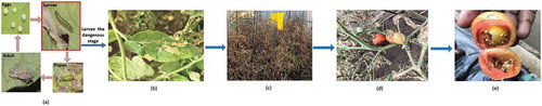
Tuta absoluta can yield up to 12 generations per year and each mature female adult can produce between 250 and 300 eggs in its lifetime (Doğanlar and Yİğİt 2011). It has four development stages (egg, larva, pupa, adult) in its life cycle, exhibited for about 26–28 days (Desneux et al. 2010). All four development stages are harmful and can attack different parts of the host plant (Guimapi et al. 2016). The larva is the most dangerous stage that usually affects plant leaves but can also be found in fruits and stems where they feed and develop, creating conspicuous mines and galleries (Cuthbertson et al. 2013). Figure 1 shows the damage caused by T. absoluta on tomatoes.

Figure 1. Tuta absoluta’s life cycle and its damage to tomatoes. (a) Four stages of T. absoluta’s life cycle. (b) Tomato leaf with T. absoluta mines. (c) Severe damage on tomato field. (d) Damaged tomato fruits in the field. (e) Damaged tomato fruit on the market

Over the years, farmers have been using different methods in efforts to control the pest unsuccessfully. These include the use of pheromone traps and natural enemies to monitor the population, cultivation of resistant tomato varieties, and incessant spraying of chemical pesticides, which is still the main control method (Guedes and Picanço 2012). The excessive use of these chemicals is not only uneconomical but also has harmful effects on non-targeted organisms and can also lead to the development of pest resistance and irreparable damage to the environment (Materu et al. 2016). Although farmers and extension officers struggle with different methods to control the pest, there has not yet been an effective mechanism to exploit the extent to which T. absoluta infected tomato leaves at early stages before causing significant yield loss to farmers.

Inspired by the advancement and promising results of Deep Learning techniques in image-based plant pest and disease diagnosis, this research proposes a model based on Convolutional Neural Networks (CNNs) for segmenting T. absoluta’s damage to tomato leaf images at pixel level. The exact location of tuta mines in plants can be obtained. This will enable farmers to make informed decisions in controlling the pest, improving tomato productivity, and rescuing them from the losses they incur annually.

Related works

Computer Vision using Deep Learning methods such as CNNs have presented promising and impressive results in diagnosing a diverse range of plant diseases and pests (Singh et al. 2018). Brahimi, Boukhalfa, and Moussaoui (2017) presented deep CNN models based on AlexNet and GoogleNet trained using a dataset of 14,828 images to automatically determine 9 diseases in tomatoes. The model attained an accuracy of 99.185%. Also, Mkonyi et al. (2020) developed a model based on VGG16, VGG19, and ResNet50 architectures to identify T. absoluta in tomato plants using a dataset of 2145 tomato leaf images. VGG16 achieved a high accuracy of 91.9%. Nevertheless, there is still a need to detect the exact location and shape of T. absoluta’s damage.

Similarly, researchers such as Ferentinos (2018), Zhang et al. (2018), Fuentes et al. (2017), and Sladojevic et al. (2016) proposed deep CNN models for detecting different diseases and pests in various plants like banana, tomato, pear, cherry, peach, apple, and grapevine using leaf image datasets.

Although the problem of plant leaf disease detection has been addressed in several studies, only a few of these have focused on developing systems capable of segmenting infected areas. K. Lin et al. (2019) proposed a segmentation model based on U-Net architecture to segment powdery mildew on cucumber, a common fungal disease that mainly infects plant leaves. A dataset of 50 cucumber leaf images captured in a cucumber fruit leaf phenotype automated analysis platform was used in their experiment. The model performed well with an averaged accuracy of 96.08% on test data, outperforming conventional Machine Learning methods, such as K-means and Random Forest.

Q. Wang et al. (2019) presented a tomato disease detection model based on Faster R-CNN and Mask RCNN. The model detects and segments the locations and shapes of the infected area on tomato fruits. In their experiment, a dataset of 286 tomato fruit images obtained from the internet was used. The models achieved mean Average Precision (mAP) of 88.53% and 99.64% for Faster R-CNN and Mask RCNN, respectively.

Also, Pérez-borrero et al. (2020) proposed a deep learning method based on Mask RCNN architecture for instance segmentation of strawberries. In their experiment, a dataset of 3100 strawberry images along with their annotations was used. They modified the Mask RCNN structure and proposed a new performance metric, the Instance Intersection Over Union (I²oU) to assess the instance segmentation. Their model achieved a mAP of 43.85% compared to 45.36% of the original Mask RCNN and the mean I²oU of 87.27% compared to 87.70% of the original Mask RCNN.

Tang, Wang, and Chen (2020) developed a dilated encoder network (DE-Net) model based on U-Net architecture for automatic butterfly ecological image segmentation. In their proposed method, the U-Net architecture was modified by replacing the last two pooling layers, the last three convolution layers and all fully connected layers with the hybrid cascade dilated convolution (HCDC) to capture deeper semantic features. A public dataset of 832 butterfly ecological images was used and the DE-Net model achieved an accuracy of 98.67%.

The study by Liu, Hu, and Li (2020) proposed a method to segment overlapped poplar seedling leaves under heavy metal stress by combining Mask RCNN with Density-Based Spatial Clustering of Applications with Noise (DBSCAN) clustering algorithm. The Mask RCNN was used to segment leaves and then DBSCAN was used to cluster single leaves from detected overlapping leaves. A dataset of 2000 RGB-D images with their corresponding annotations was used to complete the task. In their experiment, the model obtained a pixel-wise Intersection over Union (p-IoU) and mean accuracy of 0.874 and 0.888, respectively.

Generally, these studies have achieved excellent results in image-based plant diagnosis using CNNs. However, none addresses the segmentation of T. absoluta’s effects on tomato plants. Some studies also used a limited dataset size and images from online repositories that may not reflect the actual field situation. Therefore, this study proposes a deep learning-based approach for segmenting T. absoluta at the early stages of the tomato plant’s growth using images collected from the field to determine its damage.

Material and methods

The dataset

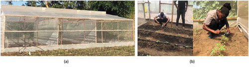
This study was conducted in Tanzania with two in-house experiments that were set up in Arusha and Morogoro regions. The two regions are the major areas on tomato production and highly prone to T. absoluta infestation. In each region, we constructed a net house and then planted healthy tomato seedlings (free from other diseases and pests) as shown in Figure 2. We inoculated T. absoluta on randomly selected tomato plants on the second day after transplanting by placing 2 to 8 larvae on top of each plant’s leaves. The pest immediately started to mine the leaves. The inhouse experiments prevented any other pests into the net house and T. absoluta from getting out of the experimental area, hence maintaining a controlled environment for the study.

Figure 2. Experimental setup in a field. (a) A nethouse. (b) Researcher and an agricultural expert performing infestation in Arusha and Morogoro fields

We collected tomato plant images using a camera. The data collection work took two weeks after infestation. The two-week period reflects the plant’s early growth stages. A dataset of 5235 tomato images was collected and manually labeled with the help of an agricultural expert. This includes 2319 and 2916 images collected in Arusha and Morogoro, respectively, as shown in Table 1. Figure 3 shows sample images from our dataset demonstrating the development of “tuta” mines on different days.

Figure 3. Some images from our dataset showing the development of tuta mines on different days

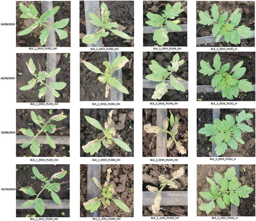
Table 1. Dataset distribution

Region	Healthy	Infested with T. absoluta	Total Number of Images
Arusha	1107	1212	2319
Morogoro	1870	1046	2916
Total	2977	2258	5235

Research framework

Figure 4 shows the research framework of our study and gives a clear understanding of how the research was undertaken from data collection to model development and validation until the delivery of an optimized model. Two deep meta-architectures, namely U-Net and Mask RCNN, were used to develop a semantic and an instance segmentation model, respectively. The segmentation model can determine the exact spot in the plant infected with T. absoluta. The model’s performance was then evaluated using different evaluation metrics and the model’s parameters are tuned to get an optimized model.

Figure 4. Research conceptual framework

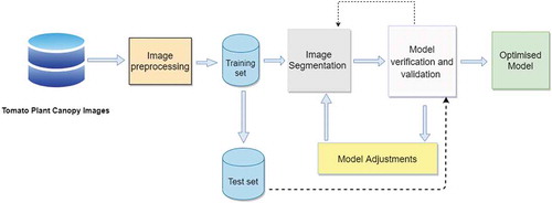
Image pre-processing

In this work, the image pre-processing involved image labeling, annotation, resizing and augmentation.

Image annotation

We selected 1212 and 1240 images of infested plants dataset to develop U-Net and Mask RCNN models respectively. For each image, a ground truth labeled image was manually generated containing the individual segmentation of all the T. absoluta’s mines present in the image. Labelme (Russell et al. 2008) and VGG Image Annotator (Dutta and Zisserman 2019), open-source tools were used to annotate images for semantic and instance segmentation tasks, respectively. The specific operation was to define the continuous contour of all T. absoluta’s mines by marking the area and shape of the infested spot with irregular polygons and then labeling the spot with “tuta.” Each image contained at least one tuta mask indicating the presence of the T. absoluta’s mine. The obtained annotations were saved in VOC (Everingham et al. 2010) and COCO (T. Lin, Zitnick, and Doll 2014) formats with their corresponding images for semantic and instance segmentation tasks, respectively. We split the annotated dataset into training and test sets in a ratio of 80:20, respectively, as shown in Table 2. The training set was used to train the model, while the test set was used to evaluate the model’s performance.

Table 2. Train/test set splits

Model	Data Ratio	Training set	Test set	Total
U-Net (VOC format)	80:20	969	243	1212
Mask RCNN (COCO format)	80:20	992	248	1240

Resizing the images

A large input image requires the neural network to learn from many pixels adding up the training time and other computational costs. Therefore, many CNN architectures require that the input images are of the same size. The images in our dataset varied in size, so we used a standard resize function in Keras to resize all images to 512 × 512 pixels.

Augmentation

Deep neural networks are data-hungry. They need a large amount of training data to achieve good performance and avoid overfitting (Lawrence and Giles 2000). Unfortunately, we were not able to collect enough data to sufficiently train a CNN model. This is because the experiment was designed to collect data for 14 days after T. absoluta infestation to analyze the effects of the pest in the early growth stages of the tomato plants. Data augmentation is a solution to the problem of limited data. Image data augmentation encompasses a suite of techniques that can be used to artificially expand the size and enhance the quality of the training dataset by creating modified versions of the original images in the dataset (Shorten and Khoshgoftaar 2019). Specifically, the following set of augmentation was applied to the training set only with data values in a range of (0, 1).

- Horizontal flip. All images were horizontally flipped with a probability of 0.5.

- Vertical flip. All images were vertically flipped with a probability of 0.2.

-Random Crop. A random crop was applied on images with the interval of (0, 0.1).

- Gaussian Blur. A gaussian blur with a probability of 0.5 was applied to images with a random sigma of between 0 and 0.5.

- Contrast Normaization. Applied to strengthen or weaken the contrast in each image in the interval (0.75, 1.5).

- Gaussian Noise. Gaussian noise with a probability of 0.5 was added to images.

- Brightness modification. A change of brightness was applied with a probability of 0.2 and a random value in the interval (0.8, 1.2) was chosen.

- Affine Transformation. Zooming/scaling images to 90 - 110% of their height/width (each axis independently). Translate/move images by -20 to +20 relative to their height/width per axis. Rotate images by -5 to +5 degrees and slightly shear them by -2to +2 degrees.

Proposed models

This work aims to develop two models based on deep CNNs to detect the regions in tomato plants infected by T. absoluta. We employed transfer learning based on the CNN models, Mask RCNN and U-Net that were trained and shown best performance on COCO (T. Lin, Zitnick, and Doll 2014) and International Symposium on Biomedical Imaging (ISBI) (Ronneberger, Fischer, and Brox 2015) datasets for instance and semantic segmentation tasks respectively.

U-net for semantic segmentation

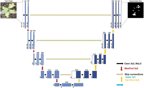
In semantic segmentation, different instances of the same object are not distinguished and are given the same label. Ronneberger, Fischer, and Brox (2015) introduced a U-shaped CNN architecture designed to be trained end-to-end with very few images and yet produce more precise segmentations. This makes it very suitable for the agricultural field since there is not enough labeled data to train complex CNN architectures in the real world (K. Lin et al. 2019). The model has performed well first in the biomedical image segmentation and later in many other fields outperforming the earlier segmentation methods (Ciresan et al. 2012). The U-Net architecture consists of three sections: an encoder, a bottleneck, and a decoder, hence the name encoder-decoder structure. The encoder down-samples the input image, captures its context, and outputs a tensor containing information about the object, its shape, and size. The decoder which has up-sampling layers takes this information and produces segmentation maps using transposed convolutions. This up-sampling process makes the network’s output the same size as the input image achieving pixel-level segmentation. The bottleneck section mediates between the encoder and decoder sections. It uses skip connections to concatenate the intermediate outputs of the encoder with the inputs to the intermediate layers of the decoder at appropriate positions. This concatenation process enables the precise localization of the target objects. The U-Net architecture is described in Figure 5.

Figure 5. U-Net architecture

Mask RCNN for instance segmentation

Mask Region-based CNN takes an input image and outputs a bounding box, label, and the corresponding mask (He et al. 2018). It is an extension of the Faster RCNN model, which has two outputs for each candidate object, a class label and a bounding-box offset (Ren et al. 2017). Mask RCNN adds a third branch that outputs the object mask, decoupling class prediction and mask generation. This makes it an effective algorithm for more challenging instance segmentation tasks. The architecture of the proposed Mask RCNN model is illustrated in Figure 6.

Figure 6. Proposed Mask RCNN model architecture

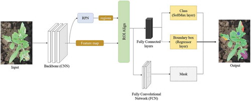
Backbone: CNN backbone architecture is used to extract features from an input image. The proposed Mask RCNN uses ResNet50 and ResNet101 for feature extraction. The extracted features act as an input for the next layer.

Region Proposal Network (RPN): The RPN is applied to the feature maps from the previous step and outputs a set of object/region proposals i.e., Regions of Interest (ROIs), each with its objectness score. RPN uses a sliding window over the convolutional feature maps producing anchor boxes of different shapes and sizes to generate region proposals. Then, for each anchor box, the RPN predicts the probability that an anchor is an object. Using the non-maximum suppression technique, the RPN refine anchors with a high objectness score and suppress or reject all other boxes.

Regions of Interest Align: Both RoIs and their corresponding feature maps from the previous step are passed through the RoI Align layer which converts them to a fixed shape and size. RoI Align uses binary interpolation to generate a small feature map of fixed size (e.g., 7 × 7) from each RoI. The RoI Align layer properly aligns the extracted features with the input and accurately maps RoIs from the original image onto the feature map without rounding up to integers.

Fully Connected Layers: On top of the fully connected network, a softmax layer is used to predict classes in the image. A linear regression layer is also used alongside the softmax layer to output bounding box coordinates for predicted classes.

Fully Convolutional Network: The output of the ROI Align layer also goes separately to the convolutional layer to predict the masks. This network takes an RoI as input and outputs the m*m mask representation. The mask shape is normally 28 × 28.

Training phase

U-net: Hyperparameters tuning and network training

A Keras U-Net architecture was used in this implementation to develop a T. absoluta semantic segmentation model. We set 32 convolutional filters in the initial convolutional block which will be doubled after every block while setting 4 total number of layers in the encoder path. To increase the convergence rate of the architecture to our dataset, we use batch normalization for each layer in our network. Since our problem is binary segmentation, we set the sigmoid as the activation function in the output layer. All images in our dataset were rescaled by 1/255 to range (0–1) then resized to 512 × 512 pixels. Since our training set contains only 969 images which are insufficient to train the network, we perform random data augmentation to expand these 969 images to train the neural network effectively. The augmentation techniques include rotation in a range of 5.0 degrees, horizontal and vertical flipping, width and height shift in a range of 0.05, shear in a range of 40, and the zoom range of 0.2. When an image is transformed, its corresponding annotation is transformed in the same way. The generated images with their corresponding annotation images are shown in Figure 7.

Figure 7. Augmented images with their corresponding annotations

We trained our networks using 200 epochs with a learning rate of 0.01 and Adam (Kingma and Ba 2014) as the optimization function. The IoU threshold for minimum detection probability is kept at 0.5.

Mask RCNN: Hyperparameters tuning and network training

Two CNN architectures, namely, ResNet50 and ResNet101, were used separately as backbone architectures of our Mask RCNN model. Since we ran inference on one image at a time, we set the batch size to 1 where each batch has 1 image per GPU. A learning rate, weight decay, and learning momentum of 0.001, 0.0001, and 0.9, respectively, have been used in this implementation. The detection minimum probability is kept at 0.7 so that RoIs with score larger than this threshold are kept and below that are skipped. The training was developed during 200 epochs and the model was evaluated on the validation set at the end of each epoch.

Loss function

U-Net Loss Function: The U-Net uses a pixel-wise cross-entropy loss that examines each pixel individually comparing it to the ground truth pixel then averaged over all pixels. This loss weighting scheme helps the U-Net model segment tuta mines in tomato leaf images in a discontinuous fashion such that individual mines can be easily identified within the binary segmentation map.

The loss is defined as

(1) $\begin{array}{c}L=\sum _{i=1}^m-\left(y_{i}log\left(p_i\right)+\left(1-y_i\right)log\left(1-p_i\right)\right)\end{array}$(1)

Where

$L$ is the total loss in U-Net.

$m$ is the number of pixels in an image.

i is the index of a pixel.

$y_i$ is the binary indicator i.e. the ground truth or real value of the i-th pixel whose value is 0 or 1.

$log$ is the natural log.

$p_i$ is the predicted probability/value of the i-th pixel. Its value ranges from 0 to 1.

Mask RCNN Loss Function: We define a multitask loss function calculated as the weighted sum of various losses at each stage of Mask RCNN model training. This comprises three (3) losses: loss due to classification, regression, and mask prediction. The regression and mask loss are only applied to positive examples.

The total loss is defined as

(2) $\begin{array}{c}{L}_{T\hspace{0.17em}}=\sum _i{L}_{cls}\left(p_i,g_i\right)+\sum _i{g}_i{L}_{reg}\left(t_i,t_i^{\ast }\right)+\sum _i{g}_i{L}_{mask}\left(m_i,m_i^{\ast }\right)\end{array}$(2)

Where

$L_T=L\left(\left\{p_i\right\},\left\{t_i\right\},\left\{m_i\right\}\right)$ is the total loss in Mask R-CNN.

i is the index of an anchor.

$p_i$ is the predicted probability of an anchor i being an object.

$g_i$ is the ground-truth probability of anchor i. Ground-truth label $g_i$ is 1 if the anchor is positive and is 0 otherwise.

$t_i=\left(t_i^x,t_i^y,t_i^h,t_i^w\right)$ is a vector with the horizontal and vertical coordinates of the center point and the height and width coordinates of the predicted bounding box.

$t_i^{\ast }$ is a vector representing four (4) parameterized coordinates (x,y,h,w) of the ground-truth bounding box associated with a positive anchor i.

$L_{cls}$ is the classification loss.

$L_{reg}$ is the regression loss. The term $g_i{L}_{reg}$ means that regression loss is only activated for positive anchors ($g_i=1$) and is disabled otherwise ($g_i=0$).

$L_{mask}$ is the mask loss. The term $g_i{L}_{mask}$ means that mask loss is only activated for positive anchors ($g_i=1$) and is disabled otherwise ($g_i=0$).

Results and discussion

Experiment settings

The experiments were conducted on a computer pre-installed with Windows 10 equipped with one Intel® Core™ i7-8550 U 3.6 GHz CPU, Intel® Iris® Plus Graphics, 512 GB SSD storage and 16 GB memory. Google Collaboratory with Tesla P100-PCIE GPU and 27GB memory was utilized. Using Python 3, Keras (Chollet 2017) library with Tensorflow (Abadi 2016) as backend, we implemented our proposed network.

Apart from detection rates, the efficiency of the model is another important performance criterion. Table 3 shows the training time in minutes of all tomato leaves images for each method employed in this study. It can be seen that the training time of U-Net is 483.50 minutes which is 169.91 and 359.45 minutes shorter than that of Mask RCNN with ResNet50 and with ResNet101 as backbones respectively. This is because the ResNet101 has a more complex structure compared to ResNet50 and U-Net hence longer training time.

Table 3. Training time

Method	Training time (minutes)
Mask RCNN-ResNet50	653.41
Mask RCNN-ResNet50 with augmentations	670.57
Mask RCNN-ResNet101	842.95
Mask RCNN-ResNet101 with augmentations	853.40
U-Net	483.50

Loss results

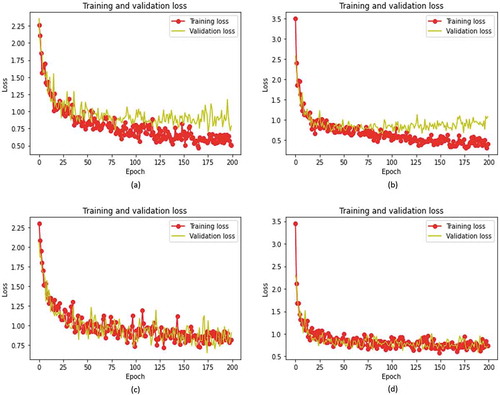
Figure 8 demonstrates the loss diagrams of the proposed model during the training process of the Mask RCNN model. The training and validation losses were estimated after each training epoch. As the training process progresses, the value of training loss rapidly decreases, followed by validation loss. As revealed in Figure 8 (a) and (b), the validation loss starts to display an upward trend after several epochs while the training loss continues to decrease, suggesting overfitting of the model. We select the last epoch that did not overfit. Then we retrain the network with augmentation techniques described in Image pre-processing section keeping a record of the total loss. A shown in Figure 8 (c) and (d), the loss function monotonically decreases during the training phase. At the end of the training, the losses are stabilized, indicating that our proposed model learns and segments the tuta mines well without overfitting.

Figure 8. Training and validation loss curve for Mask RCNN. Loss graph for (a) Mask RCNN-ResNet50, (b) Mask RCNN-ResNet101, (c) Mask RCNN-Resnet50 with augmentations, and (d) Mask RCNN-Resnet101 with augmentations

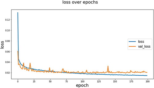
On the other hand, Figure 9 illustrates the training loss curve of U-Net with 200 epochs. We can see the losses dropped rapidly during early training iterations then start to stabilize at about 50 epochs which implies that the model fits well on the features of our dataset at early and later stages of the training process. In theory, the U-Net model has the best performance since it eventually obtains the lowest loss value compared to Mask RCNN.

Figure 9. Training and validation loss curve for U-Net

Evaluation metrics

In this paper, we analyzed the quality of the semantic segmentation results of our model using Intersection over Union and dice coefficient. On the other hand, precision, recall and mAP are the performance metrics selected for validation of the proposed instance segmentation model.

The equations for evaluating the proposed semantic segmentation model are shown in Eqs 3(3) $\begin{array}{c}IoU=\frac{\begin{array}{c}\hspace{0.17em}\\ OverlappingArea\end{array}}{\begin{array}{c}UnionArea\\ \hspace{0.17em}\end{array}}\end{array}$(3) and 4(4) $\begin{array}{c}DiceCoefficient=\frac{2\times Intersection}{Union+Intersection}\end{array}$(4) .

(3) $\begin{array}{c}IoU=\frac{\begin{array}{c}\hspace{0.17em}\\ OverlappingArea\end{array}}{\begin{array}{c}UnionArea\\ \hspace{0.17em}\end{array}}\end{array}$(3)

(4) $\begin{array}{c}DiceCoefficient=\frac{2\times Intersection}{Union+Intersection}\end{array}$(4)

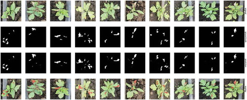
Figure 10 shows the results of the metrics used to evaluate the performance of the proposed model based on U-Net architecture. The model achieved satisfactory accuracy in segmenting T. absoluta’s mines in tomato plants. As shown, the U-Net model obtained a dice coefficient and an IoU of 82.86% and 78.60% respectively. The value of the dice coefficient is usually greater than that of IoU in the same segmentation performance. Some examples of the segmentations carried out by the proposed U-Net model are shown in Figure 11. As can be observed, the model generates precise segmentations of tuta mines in tomato plants.

Figure 10. The evaluation metrics results for the semantic segmentation model. (a) IoU for U-Net. (b) Dice Coefficient for U-Net

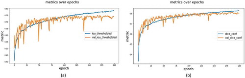
Figure 11. Examples of segmentations carried out by the proposed U-Net model

Precision: measures the percentage of correct positive predictions among all predictions made. Recall: measures the percentage of correct positive predictions among all actual positive cases. The two metrics are calculated as follows:

(5) $\begin{array}{c}Precision=\frac{TP}{TP+FP}\end{array}$(5)

(6) $\begin{array}{c}Recall=\frac{TP}{TP+FN}\end{array}$(6)

Where

$TP$ is the number of positive samples correctly predicted to be positive, i.e., the number of correctly detected tuta mines.

$FP$ is the number of negative samples that are wrongly predicted as positive i.e the number of falsely detected tuta mines.

$FN$ (False Negative) is the number of negative samples that are correctly predicted as negative. i.e the number of missed tuta mines.

Mean Average Precision: is used as the primary evaluation metric to measure the quality of the segmentations obtained by the model. It provides the average precision of object locations in all predictions matching ground-truth objects giving each object equal importance.

mAP is defined as

(7) $\begin{array}{c}mAP=\frac{1}{N}\sum AP\end{array}$(7)

Where

$mAP$ is the mean Average Precision of all classes.

$AP$ is the Average Precision.

$\sum AP$ is the sum of the Average Precision values.

$N$ is the number of all classes.

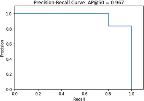
The area under the Precision-Recall (PR) curve which defines the Average Precision (AP) can be used to summarize the performance of a segmentation model; the x-axis being recall and the y-axis being precision. We set a threshold of IoU = 0.5 at which any segmentation with a score lower than this value is treated as a FP. As shown in Figure 12 the PR curve is monotonically decreasing which is what we want for better performance. The precision of a detector with good performance remains high as recall increases, which means it will detect a high proportion of TP before it starts detecting FP.

Figure 12. The Precision-Recall Curve

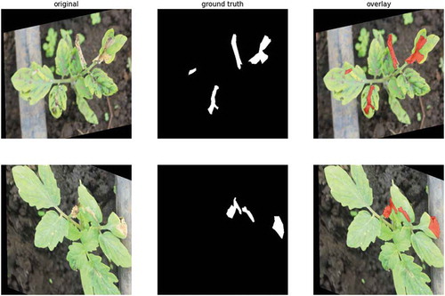
Table 4 summarizes mAP values measuring the performance of the proposed methods in detecting and segmenting tuta mines on tomato images. The mAP value of Mask RCNN-ResNet50 with augmentations is as high as 85.67%, achieving the highest detection rates on tuta mines in tomato plants compared to other methods. As can be seen from the table, the performance of Mask RCNN-ResNet50 and Mask RCNN-ResNet101 are relatively poor with an mAP of 81.01% and 81.09% respectively, possibly because of the complexity of backbone architectures to train on an insufficient amount of data. Examples of segmentations performed by the proposed Mask RCNN model are shown in Figure 13. As can be observed, the model could detect even the smallest tuta mines on tomato leaves.

Figure 13. Examples of segmentations carried out by the proposed Mask RCNN model

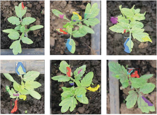
Table 4. The mAP (primary metric) values of the tomato images obtained by different detection methods

Method(s)	mAP (%)
Mask RCNN-ResNet50	81.01
Mask RCNN-ResNet50 with augmentations	85.67
Mask RCNN-ResNet101	81.09
Mask RCNN-ResNet101 with augmentations	82.72

Conclusion and future work

This paper aimed to tackle the problem of accurately segmenting T. absoluta’s damage on tomato plants at their early growth stage. To address this problem, this novel work proposed deep CNN models based on U-Net and Mask RCNN architectures which are used for automatic semantic and instance segmentations, respectively. The experimental results indicate that the Mask RCNN-ResNet50 model performs best in segmenting tuta mines in tomato leaf images, achieving an mAP of 85.67%, while the U-Net model obtained an IoU of 78.60% and a dice coefficient of 82.86%. Both proposed models were very precise in segmenting the shapes of the areas infected by T. absoluta in tomato leaves. This demonstrates that deep learning is the promising technological approach for fully automatic and early determination of T. absoluta’s damage. This novel work contributes to the body of knowledge and can help farmers and extension officers to make informed decisions that could improve tomato productivity and rescue farmers from the losses they incur annually.

However, it is worth noting that there are some limitations to this study. The experiments used insufficient annotated dataset size that considered T. absoluta only, leaving out other pests and diseases and also had a limited computing power, factors that may affect the performance of the model. Even though this study has achieved excellent segmentation results, adding more annotated data could further improve the performance of the proposed models.

In the future, we expect to develop a CNN quantification model and decision support system that will be deployed in a mobile or computer to enable farmers and extension officers to make intelligently informed decisions on how to control the pest. The system will be able to count the leaves, determine the extent of damage and suggest actions to be taken such as Integrated Pest Management (IPM) techniques to control the pest based on the estimated severity. To facilitate further research in diagnosing T. absoluta’s damage to tomato plants, the dataset associated with this work is freely available to the research community and can be accessed at the open access repository (Rubanga et al. 2020).

Disclosure Statement

The authors declare that there are no conflicts of interest regarding the publication of this paper.

Correction Statement

This article has been republished with minor changes. These changes do not impact the academic content of the article.

Additional information

Funding

This work was supported by the African Development Bank (AfDB) through Project No. P-Z1-IA0-016 under Grant No. 2100155032816.

References

- Abadi, M. 2016. TensorFlow: learning functions at scale. In Proceedings of the 21st ACM SIGPLAN International Conference on Functional Programming 51(9):1–1. Nara, Japan: Association for Computing Machinery. 10.1145/3022670.2976746
- Brahimi, M., K. Boukhalfa, and A. Moussaoui. 2017. Deep learning for tomato diseases: classification and symptoms visualization. Applied Artificial Intelligence 31 (4):299–315. doi:https://doi.org/10.1080/08839514.2017.1315516.
- Chollet, F. 2017. Introduction to keras. In Deep learning with python. 1st ed. 60–62. New York:Manning Publications Co.
- Ciresan, D. C., A. Giusti, L. M. Gambardella, and J. Schmidhuber. 2012. Deep neural networks segment neuronal membranes in electron microscopy images. Advances in Neural Information Processing Systems 25: 2843–2851
- Cuthbertson, A. G. S., J. J. Mathers, L. F. Blackburn, A. Korycinska, W. Luo, R. J. Jacobson, and P. Northing. 2013. Population development of tuta absoluta (meyrick) (lepidoptera: gelechiidae) under simulated UK glasshouse conditions. Insects 4 (2):185–97. doi:https://doi.org/10.3390/insects4020185.
- Desneux, N., E. Wajnberg, K. A. G. Wyckhuys, G. Burgio, S. Arpaia, C. A. Narváez-Vasquez, J. González-Cabrera, D. C. Ruescas, E. Tabone, J. Frandon, et al. 2010. Biological invasion of european tomato crops by tuta absoluta: ecology, geographic expansion and prospects for biological control. Journal of Pest Science 83 (3):197–215. doi:https://doi.org/10.1007/s10340-010-0321-6.
- Doğanlar, M., and A. Yİğİt. 2011. Parasitoids complex of the tomato leaf miner, tuta absoluta (meyrick 1917), (lepidoptera: gelechiidae) in Hatay Turkey. KSU Journal of Natural Sciences 14 (4):28–37. doi:https://doi.org/10.18016/ksujns.36297.
- Dutta, A., and A. Zisserman. 2019. The VIA annotation software for images, audio and video. In Proceedings of the 27th ACM International Conference on Multimedia (MM '19), 2276–79. Nice, France: Association for Computing Machinery, Inc. doi: https://doi.org/10.1145/3343031.3350535
- Everingham, M., L. V. Gool, C. K. I. Williams, and J. Winn. 2010. The PASCAL Visual Object Classes (VOC) challenge. International Journal of Computer Vision 88 (2):303–38. doi:https://doi.org/10.1007/s11263-009-0275-4.
- FAOSTAT. 2019. Tomato production worldwide. Food and Agriculture Organization (FAO). Accessed March 27, 2020. http://www.fao.org/faostat/en/?#data/QC.
- Ferentinos, K. P. 2018. Deep learning models for plant disease detection and diagnosis. Computers and Electronics in Agriculture 145 (January):311–18. doi:https://doi.org/10.1016/j.compag.2018.01.009.
- Fuentes, A., S. Yoon, S. C. Kim, and D. S. Park. 2017. A robust deep-learning-based detector for real-time tomato plant diseases and pests recognition. Sensors 17 (9):9. doi:https://doi.org/10.3390/s17092022.
- Guedes, R. N. C., and M. C. Picanço. 2012. The tomato borer tuta absoluta in south America: Pest status, management and insecticide resistance. EPPO Bulletin 42 (2):211–16. doi:https://doi.org/10.1111/epp.2557.
- Guimapi, R. Y. A., S. A. Mohamed, G. O. Okeyo, F. T. Ndjomatchoua, S. Ekesi, and H. E. Z. Tonnang. 2016. Modeling the risk of invasion and spread of tuta absoluta in Africa. Ecological Complexity 28:77–93. doi:https://doi.org/10.1016/j.ecocom.2016.08.001.
- He, K., G. Gkioxari, P. Dollár, and R. Girshick. 2018. Mask R-CNN. IEEE Transactions on Pattern Analysis and Machine Intelligence 42 (2):386–97. doi:https://doi.org/10.1109/TPAMI.2018.2844175.
- Kingma, D. P., and J. Ba. 2014. Adam: A method for stochastic optimization. arXiv preprint arXiv:1412.6980.
- Lawrence, S., and C. L. Giles. 2000. Overfitting and neural networks: conjugate gradient and backpropagation. Proceedings of the IEEE-INNS-ENNS International Joint Conference on Neural Networks. IJCNN 2000. Neural Computing: New Challenges and Perspectives for the New Millennium 1: 114–19. IEEE. doi: https://doi.org/10.1109/IJCNN.2000.857823.
- Lin, K., L. Gong, Y. Huang, C. Liu, and J. Pan. 2019. Deep learning-based segmentation and quantification of cucumber powdery mildew using convolutional neural network. Frontiers in Plant Science 10 (February):1–10. doi:https://doi.org/10.3389/fpls.2019.00155.
- Lin, T., M. Maire, S. Belongie, J. Hays, P. Perona, D. Ramanan, P. Dollár, and C. L. Zitnick. 2014. Microsoft COCO: Common objects in context. European Conference on Computer Vision, ed. D. Fleet, T. Pajdla, B. Schiele, and T. Tuytelaars, 8693: 740–755. Cham, Switzerland: Springer International Publishing. doi: https://doi.org/10.1007/978-3-319-10602-1_48.
- Liu, X., C. Hu, and P. Li. 2020. Automatic segmentation of overlapped poplar seedling leaves combining mask R-CNN and DBSCAN. Computers and Electronics in Agriculture 178 (May):105753. doi:https://doi.org/10.1016/j.compag.2020.105753.
- Maneno, C., S. Al-zaidi, N. Hassan, J. Abisgold, E. Kaaya, and S. Mrogoro. 2016. First record of tomato leafminer tuta absoluta meyrick (lepidoptera: Gelechiidae) in Tanzania. Agriculture & Food Security 5 (1):17. doi:https://doi.org/10.1186/s40066-016-0066-4.
- Materu, C. L., E. A. Shao, E. Losujaki, and M. Chidege. 2016. Farmer’s perception knowledge and practices on management of tuta absoluta meyerick (lepidotera gelechiidae) in tomato growing areas in Tanzania. International Journal of Research in Agriculture and Forestry 3 (2):1–5.
- Mkonyi, L., D. Rubanga, M. Richard, N. Zekeya, S. Sawahiko, B. Maiseli, and D. Machuve. 2020. Early identification of tuta absoluta in tomato plants using deep learning. Scientific African 10:e00590. doi:https://doi.org/10.1016/j.sciaf.2020.e00590.
- Mutayoba, V., and D. Ngaruko. 2018. Assessing tomato farming and marketing among smallholders in high potential agricultural areas of tanzania. International Journal of Economics, Commerce and Management (IJECM) VI (8):577–90.
- Never, Z., P. A. Ndakidemi, M. Chacha, and E. Mbega. 2017. Tomato leafminer, tuta absoluta (meyrick 1917), an emerging agricultural pest in sub-saharan Africa: Current and prospective management strategies. African Journal of Agricultural Research 12 (6):389–96. doi:https://doi.org/10.5897/AJAR2016.11515.
- Pérez-borrero, I., D. Marín-santos, M. E. Gegúndez-Arias, and E. Cortés-Ancos. 2020. A fast and accurate deep learning method for strawberry instance segmentation. Computers and Electronics in Agriculture 178 (February):105736. doi:https://doi.org/10.1016/j.compag.2020.105736.
- Ren, S., K. He, R. Girshick, and J. Sun. 2017. Faster R-CNN: Towards real-time object detection with region proposal networks. IEEE Transactions on Pattern Analysis and Machine Intelligence 39 (6):1137–49. doi:https://doi.org/10.1109/TPAMI.2016.2577031.
- Ronneberger, O., P. Fischer, and T. Brox. 2015. U-net: Convolutional networks for biomedical image segmentation. In International Conference on Medical Image Computing and Computer-Assisted Intervention - MICCAI 2015, ed. N. Navab, J. Hornegger, W. M. Wells and A. F. Frangi, 9351:234–241. Cham, Switzerland: Springer. https://doi.org/10.1007/978-3-319-24574-4_28.
- Rubanga, D. P., L. Mkonyi, M. Richard, N. Zekeya, L. K. Loyani, S. Shimada, and D. Machuve. 2020. A deep learning dataset for tomato pest leafminer TUTA ABSOLUTA. Zenodo Repository. Accessed December 6:2020. doi:https://doi.org/10.5281/ZENODO.4305416.
- Russell, B. C., A. Torralba, K. P. Murphy, and W. T. Freeman. 2008. LabelMe : A database and web-based tool for image annotation. International Journal of Computer Vision 77 (1–3):157–173.
- Shorten, C., and T. M. Khoshgoftaar. 2019. A survey on image data augmentation for deep learning. Journal of Big Data 6 (1):1. doi:https://doi.org/10.1186/s40537-019-0197-0.
- Singh, A. K., B. Ganapathysubramanian, S. Sarkar, and A. Singh. 2018. Deep learning for plant stress phenotyping: trends and future perspectives. Trends in Plant Science 23 (10):883–98. doi:https://doi.org/10.1016/j.tplants.2018.07.004.
- Sladojevic, S., M. Arsenovic, A. Anderla, D. Culibrk, and D. Stefanovic. 2016. Deep neural networks based recognition of plant diseases by leaf image classification. Computational Intelligence and Neuroscience 2016:11. doi:https://doi.org/10.1155/2016/3289801.
- Tang, H., B. Wang, and X. Chen. 2020. Deep learning techniques for automatic butterfly segmentation in ecological images. Computers and Electronics in Agriculture 178 (May):105739. doi:https://doi.org/10.1016/j.compag.2020.105739.
- Tomato News. 2020. The global tomato processing industry. The Tomato Online Conference. Last Modified August 10, 2020. Accessed January 16, 2021. http://www.tomatonews.com/en/background_47.html.
- Wang, Q., F. Qi, M. Sun, J. Qu, and J. Xue. 2019. Identification of tomato disease types and detection of infected areas based on deep convolutional neural networks and object detection techniques. Computational Intelligence and Neuroscience 2019. doi:https://doi.org/10.1155/2019/9142753.
- Zekeya, N., M. Chacha, P. Ndakidemi, C. Materu, M. Chidege, and E. Mbega. 2016. Tomato leafminer (tuta absoluta meyrick 1917): A threat to tomato production in Africa. Journal of Agriculture and Ecology Research International 10 (1):1–10. doi:https://doi.org/10.9734/jaeri/2016/28886.
- Zhang, K., Q. Wu, A. Liu, and X. Meng. 2018. Can deep learning identify tomato leaf disease? Advances in Multimedia 2018. doi:https://doi.org/10.1155/2018/6710865.