Fuzzy Interpretation of the Discharge Coefficient for the Orifice Plate of Automated Flow Rate Measuring Systems

ABSTRACT

Differential pressure flowmeters play a key role in the organization of flow rate measurements of liquids and gases in various industries. Therefore, the tasks related to improving their accuracy and the convenience of forming various dependencies between the values on which the accuracy of flow rate measurement depends are very important. One of the main characteristics that determines the correct and accurate operation of differential pressure flowmeters is the discharge coefficient. In this paper, the authors present a methodology that allows us to present this coefficient as a fuzzy model. The paper presents an original method for modeling the existing discharge coefficient in the form of a fuzzy model that is able to change the existing classical equation. A comparative analysis of the fuzzy and classical models is performed for this discharge coefficient. The article analyzes the errors of the fuzzy model for the discharge coefficient, discusses ways how to reduce the error of the fuzzy model. The proposed methodology describes the application of the fuzzy model for this coefficient within the existing limits for the Reynolds number and diameter ratio. It is shown that for a more accurate approximation of the characteristics, it is necessary to add more fuzzy sets. The present method is feasible for diameter ratio $0,2\le \beta \le 0,75$ and Reynolds number greater than 5000. The article also discusses the possibilities of using fuzzy models to improve the characteristics of differential pressure flow meters.

Introduction

The problem of saving water resources and energy carriers is becoming more significant and acute in many countries of the world every year. Methods and systems of energy accounting play a special role in solving this problem. Ways to improve their accuracy and reliability also play an important role in this issue. Without reliable and accurate flow rate measuring systems of energy resources, this problem cannot be solved. Lack of accounting is the lack of control over an expensive energy carrier, which leads to its irrational use and losses. As a result, this leads to unstable and unreliable relationships between consumers and energy suppliers, overpayment for under-supplied resources, and distortion of economic indicators. Therefore, improving the means and systems for measuring the flow rate and quantity of liquids and gases is an important task in ensuring energy efficiency. There are a huge number of methods and techniques for measuring the flow and quantity of substances that implement solutions to the existing problem of organizing accurate and reliable accounting. Among a large number of methods for measuring the flow rate and quantity of liquids and gases, a special role is played by differential pressure flowmeters (Ahmed and Ghanem 2020; Baker, Lau, and Tawackolian 2013; Dayev et al. 2021; Farsi et al. 2021; Gallagher 2007; LaNasa and Upp 2014). The most common application of this method is in the gas industry. This method is often used for commercial accounting quantity of natural gas (ISO 5167–1 2003; Kremlevsky 2002).

The organization of the process of measuring the flow rate of liquids and gases with differential pressure flowmeters is described in detail in the sources (Dayev et al. 2021; ISO 5167–1 2003; Kremlevsky 2002; Reader-Harris 2015). The flow rate of a gas or liquid is highly dependent on a characteristic called the discharge coefficient. The discharge coefficient of orifice plate is calculated by the following formula (Gallagher 2007; Reader-Harris 2015):

(1) $C_d=\frac{Q\sqrt{1-{\beta }^4}}{F\epsilon \sqrt{2\mathrm{\Delta }p\rho }},$(1)

where $Q-$ actual gas mass flow rate, $\beta -$ diameter ratio, $F-$ the cross-sectional area of the orifice plate, $\epsilon -$ expansion coefficient, $\mathrm{\Delta }p-$ differential pressure on the flow transducer, $\rho -$ gas density. Equation (1)(1) $C_d=\frac{Q\sqrt{1-{\beta }^4}}{F\epsilon \sqrt{2\mathrm{\Delta }p\rho }},$(1) is not used to calculate the discharge coefficient, because there are limitations and errors for its application. Therefore, this coefficient is calculated separately by empirical equations for various types of flow transducers.

For calculation of the expansion coefficient in equation (1)(1) $C_d=\frac{Q\sqrt{1-{\beta }^4}}{F\epsilon \sqrt{2\mathrm{\Delta }p\rho }},$(1) , the following formula is used for all permitted types of pressure tapping (ISO 5167–1 2003; Pistun and Lesovoi 2005; Reader-Harris 2015):

$\epsilon =1-(0,351+0,256{\beta }^4+0,93{\beta }^8)\left[1-{\left(1-\frac{\mathrm{\Delta }p}{p}\right)}^{\frac{1}{\gamma }}\right],$

where $\gamma -$ adiabatic coefficient. The last equation is applied when the previous conditions are met for Reynolds number, diameter ratio, pipe and orifice plate diameters and the following ratio, which takes into account the compressibility of the medium:

$\mathrm{\Delta }p/p\le 0,25.$

The importance of the discharge coefficient in the organization of flow rate measurement is confirmed by a large number of publications. Historically, the first equation to calculate the discharge coefficient was published in (Stolz 1978). Further, this work was continued in work (Cristancho et al. 2010). The last equation was obtained by Reader–Harris and Gallagher. In accordance with (Cristancho et al. 2010), the values of the discharge coefficient are calculated using the following formula:

(2) $\begin{array}{rl}& C_d=0,5961+0,0261{\beta }^2-0,216{\beta }^8+0,000521{\left(\frac{{10}^6\beta }{Re}\right)}^{0.7}+\\ & +\left(0,0188+0,0063A\right){\beta }^{3,5}{\left(\frac{{10}^6}{Re}\right)}^{0,3}+\left(0,043+0,08e^{-10L_1}-0,123e^{-7L_1}\right)\times \\ & \times \left(1-0,11A\right)\frac{{\beta }^4}{1-{\beta }^4}-0,031\left(M_2-0,8M_2^{1,1}\right){\beta }^{1,3}+M_3,\end{array}$(2)

where $A={\left(\frac{19000\beta }{Re}\right)}^{0,8},$ $M_2=\frac{2L_2}{1-\beta },$

$M_3=\left\{\begin{array}{c}0{,}^{\hspace{0.17em}}D\ge 0,07112\\ 0,011\left(0,75-\beta \right)\left(2,8-\frac{D}{0,0254}\right){,}^{\hspace{0.17em}}D<0,07112\end{array}\right.$

,

$Re-$ Reynolds number, $D-$ inner diameter of pipe, the values of the coefficients L₁ and L₂ are calculated depending on the method of pressure selection (ISO 5167–1 2003). The graphical representation of equation (2)(2) $\begin{array}{rl}& C_d=0,5961+0,0261{\beta }^2-0,216{\beta }^8+0,000521{\left(\frac{{10}^6\beta }{Re}\right)}^{0.7}+\\ & +\left(0,0188+0,0063A\right){\beta }^{3,5}{\left(\frac{{10}^6}{Re}\right)}^{0,3}+\left(0,043+0,08e^{-10L_1}-0,123e^{-7L_1}\right)\times \\ & \times \left(1-0,11A\right)\frac{{\beta }^4}{1-{\beta }^4}-0,031\left(M_2-0,8M_2^{1,1}\right){\beta }^{1,3}+M_3,\end{array}$(2) is shown in Figure 1.

Figure 1. Dependence of the discharge coefficient on the number of Re

There are limitations to the application of equation (2)(2) $\begin{array}{rl}& C_d=0,5961+0,0261{\beta }^2-0,216{\beta }^8+0,000521{\left(\frac{{10}^6\beta }{Re}\right)}^{0.7}+\\ & +\left(0,0188+0,0063A\right){\beta }^{3,5}{\left(\frac{{10}^6}{Re}\right)}^{0,3}+\left(0,043+0,08e^{-10L_1}-0,123e^{-7L_1}\right)\times \\ & \times \left(1-0,11A\right)\frac{{\beta }^4}{1-{\beta }^4}-0,031\left(M_2-0,8M_2^{1,1}\right){\beta }^{1,3}+M_3,\end{array}$(2) , which is used to calculate the discharge coefficient. In accordance with the studies (Cristancho et al. 2010; Pistun and Lesovoi 2005; Reader-Harris 2015; Reader-Harris, Sattary, and Spearman 1995) and the regulatory document (ISO 5167–1 2003), the following limitations are adopted for the orifice plates. The orifice plates with angular and three-radius pressure tapping can be used under the following conditions:

$\begin{array}{rl}& d\ge 0,{0125}_{\hspace{0.17em}}(m);\\ & 0,{05}_{\hspace{0.17em}}(m)\le D\le 1,0_{\hspace{0.17em}}(m);\\ & 0,1\le \beta \le 0,75;\\ & Re\ge 5000{,}_{\hspace{0.17em}}\beta \le 0,56;\\ & Re\ge 16000{\beta }^2{,}_{\hspace{0.17em}}\beta >0,56.\end{array}$

The orifice plates with flanged pressure tapping can be used under the following conditions:

$\begin{array}{rl}& d\ge 0,{0125}_{\hspace{0.17em}}(m);\\ & 0,{05}_{\hspace{0.17em}}(m)\le D\le 1,0_{\hspace{0.17em}}(m);\\ & 0,1\le \beta \le 0,75;\\ & Re\ge 5000{,}_{\hspace{0.17em}}Re>1,7\cdot {10}^5{\beta }^{2}D.\end{array}$

An alternative representation of the discharge coefficient and the continuation of research in this area have been proposed in the works (Baker, Lau, and Tawackolian 2013; Cristancho et al. 2010; Daev 2015; Reader-Harris, Barton, and Hodges 2012; Reader-Harris and Sattary 1990; Reader-Harris, Sattary, and Spearman 1995; Reader-Harris, Sattary, and Spearman 1992a; Reader-Harris, Sattary, and Spearman 1992b). As can be seen from equation (2)(2) $\begin{array}{rl}& C_d=0,5961+0,0261{\beta }^2-0,216{\beta }^8+0,000521{\left(\frac{{10}^6\beta }{Re}\right)}^{0.7}+\\ & +\left(0,0188+0,0063A\right){\beta }^{3,5}{\left(\frac{{10}^6}{Re}\right)}^{0,3}+\left(0,043+0,08e^{-10L_1}-0,123e^{-7L_1}\right)\times \\ & \times \left(1-0,11A\right)\frac{{\beta }^4}{1-{\beta }^4}-0,031\left(M_2-0,8M_2^{1,1}\right){\beta }^{1,3}+M_3,\end{array}$(2) , the discharge coefficient is an equation of two variables Re and $\beta$, so in order to improve the methods of representation and calculation of this coefficient, other methods are being used to calculate it.

For example, in (Daev 2016; Daev and Kairakbaev 2017), the authors show the possibility of changing this coefficient under other operating conditions of differential pressure flowmeters. In (Daev and Kairakbaev 2017), the effect of straightening jets on the calculation of this coefficient is shown, and in (Daev 2016) it is shown that the presence of pulsations in the flow leads to the appearance of an additional variable in the form of the Strouhal number. In research (Dayev 2020; Dayev and Yuluyev 2019), one of the authors shows the possibility of representing this coefficient in the form of an artificial neural network, which can also be implemented in flow computers.

Taking into account that this coefficient in normal operation of variable differential pressure flow meters is a function of two variables in accordance with formula (2), in this article the authors aim to present a fuzzy interpretation of this coefficient. The authors hope that a fuzzy representation of the flow rate in the future will allow us to achieve simpler and better ways to model it in order to improve the differential pressure flowmeters accuracy. The analysis of expression (2) shows that this equation is nonlinear and quite complex for perception, therefore, according to the authors, the application of soft calculations such as fuzzy logic and modeling methods, would contribute in the future to obtain simpler and accurate methods of modeling and representation of the discharge coefficient. The importance of using fuzzy methods for modeling such characteristics of flowmeters is due to the fact that fuzzy methods are able to approximate almost any curves with very simple techniques (Kosko 1994; Piegat 2010; Yarushkina 2009). The application of new approaches expands the search for simpler methods of describing the characteristics of flowmeters, as well as contributes to the development of systems for measuring the flow rate of liquids and gas in General.

Analysis of the discharge coefficient

Equation (2)(2) $\begin{array}{rl}& C_d=0,5961+0,0261{\beta }^2-0,216{\beta }^8+0,000521{\left(\frac{{10}^6\beta }{Re}\right)}^{0.7}+\\ & +\left(0,0188+0,0063A\right){\beta }^{3,5}{\left(\frac{{10}^6}{Re}\right)}^{0,3}+\left(0,043+0,08e^{-10L_1}-0,123e^{-7L_1}\right)\times \\ & \times \left(1-0,11A\right)\frac{{\beta }^4}{1-{\beta }^4}-0,031\left(M_2-0,8M_2^{1,1}\right){\beta }^{1,3}+M_3,\end{array}$(2) is a function of two variables. On the other hand, equation (2)(2) $\begin{array}{rl}& C_d=0,5961+0,0261{\beta }^2-0,216{\beta }^8+0,000521{\left(\frac{{10}^6\beta }{Re}\right)}^{0.7}+\\ & +\left(0,0188+0,0063A\right){\beta }^{3,5}{\left(\frac{{10}^6}{Re}\right)}^{0,3}+\left(0,043+0,08e^{-10L_1}-0,123e^{-7L_1}\right)\times \\ & \times \left(1-0,11A\right)\frac{{\beta }^4}{1-{\beta }^4}-0,031\left(M_2-0,8M_2^{1,1}\right){\beta }^{1,3}+M_3,\end{array}$(2) is a strongly nonlinear dependence in order to represent it by fuzzy modeling methods. To solve such a problem, equation (2)(2) $\begin{array}{rl}& C_d=0,5961+0,0261{\beta }^2-0,216{\beta }^8+0,000521{\left(\frac{{10}^6\beta }{Re}\right)}^{0.7}+\\ & +\left(0,0188+0,0063A\right){\beta }^{3,5}{\left(\frac{{10}^6}{Re}\right)}^{0,3}+\left(0,043+0,08e^{-10L_1}-0,123e^{-7L_1}\right)\times \\ & \times \left(1-0,11A\right)\frac{{\beta }^4}{1-{\beta }^4}-0,031\left(M_2-0,8M_2^{1,1}\right){\beta }^{1,3}+M_3,\end{array}$(2) must be represented as a simple dependence of two separate independent functions, each of which depends on only one variable. To build a successful fuzzy model for this coefficient, we need to obtain simpler dependencies. These dependencies should reflect the relationship between the variables in the form of separate equations with one variable. In this case, we will be able to build a simple and effective model in the form of a MIMO-system. Therefore, it is necessary to divide equation (2)(2) $\begin{array}{rl}& C_d=0,5961+0,0261{\beta }^2-0,216{\beta }^8+0,000521{\left(\frac{{10}^6\beta }{Re}\right)}^{0.7}+\\ & +\left(0,0188+0,0063A\right){\beta }^{3,5}{\left(\frac{{10}^6}{Re}\right)}^{0,3}+\left(0,043+0,08e^{-10L_1}-0,123e^{-7L_1}\right)\times \\ & \times \left(1-0,11A\right)\frac{{\beta }^4}{1-{\beta }^4}-0,031\left(M_2-0,8M_2^{1,1}\right){\beta }^{1,3}+M_3,\end{array}$(2) by separate functions of one variable, multiplication of which gives the result in the form of the value of the discharge coefficient.

The latter problem is easily solved if we present the discharge coefficient as a dot product of the following two vectors:

(3) $C_d=\overrightarrow{f(\beta )}\cdot \overrightarrow{g(Re)},$(3)

where each of the vectors, is a five-dimensional vector with coordinates in the form of functional expressions from each variable. This application of the dot product allows us not only to simplify equation (2)(2) $\begin{array}{rl}& C_d=0,5961+0,0261{\beta }^2-0,216{\beta }^8+0,000521{\left(\frac{{10}^6\beta }{Re}\right)}^{0.7}+\\ & +\left(0,0188+0,0063A\right){\beta }^{3,5}{\left(\frac{{10}^6}{Re}\right)}^{0,3}+\left(0,043+0,08e^{-10L_1}-0,123e^{-7L_1}\right)\times \\ & \times \left(1-0,11A\right)\frac{{\beta }^4}{1-{\beta }^4}-0,031\left(M_2-0,8M_2^{1,1}\right){\beta }^{1,3}+M_3,\end{array}$(2) , but also to perform a detailed analysis of this equation. The latter opens up more opportunities for us to study the properties of the discharge coefficient, as well as to find simpler and more productive models that are based on modern techniques.

A five-dimensional vector representing the dependence of the coefficient on the diameter ratio is as follows:

$\overline{f(\beta )}=\left(\begin{array}{c}{f}_1(\beta )\\ f_2(\beta )\\ f_3(\beta )\\ f_4(\beta )\\ f_5(\beta )\end{array}\right),$

where

$f_2(\beta )={10}^{1,3}{\beta }^{3,5};$

$f_3(\beta )=0,000521\cdot {10}^{4,2}{\beta }^{0,7};$ $f_4(\beta )=-0,11\cdot {19000}^{0,8}\left(0,043+0,08e^{-10L_1}-0,123e^{-7L_1}\right)\frac{{\beta }^{4,8}}{1-{\beta }^4};$

$f_5(\beta )={10}^{1,3}{\beta }^{4,3}.$

A five-dimensional vector representing the dependence of the coefficient on the Reynolds number is as follows:

$\overline{g(Re)}={\left(\begin{array}{c}{g}_1(Re)\\ g_2(Re)\\ g_3(Re)\\ g_4(Re)\\ g_5(Re)\end{array}\right)}^T,$

where

$g_1(Re)=1;$

$g_2(Re)=0,0188\cdot {10}^{0,5}{Re}^{-0,3};$

$g_3(Re)={Re}^{-0,7};$

$g_4(Re)={Re}^{-0,8};$

$g_5(Re)=0,0063\cdot {10}^{0,5}{19000}^{0,8}{Re}^{-1,1}.$

The decomposition of equation (2)(2) $\begin{array}{rl}& C_d=0,5961+0,0261{\beta }^2-0,216{\beta }^8+0,000521{\left(\frac{{10}^6\beta }{Re}\right)}^{0.7}+\\ & +\left(0,0188+0,0063A\right){\beta }^{3,5}{\left(\frac{{10}^6}{Re}\right)}^{0,3}+\left(0,043+0,08e^{-10L_1}-0,123e^{-7L_1}\right)\times \\ & \times \left(1-0,11A\right)\frac{{\beta }^4}{1-{\beta }^4}-0,031\left(M_2-0,8M_2^{1,1}\right){\beta }^{1,3}+M_3,\end{array}$(2) as the dot product of two vectors (3) facilitates the analysis, and makes it possible to present the expression for the discharge coefficient as a fuzzy model. Figure 2 shows graphs of functions that make up the vector that depends on the diameter ratio of the orifice plate. The graphs in Figure 2 allow us to perform a detailed analysis of the dependence of the discharge coefficient on the relative diameter. The graphs clearly show that the function $f_1(\beta )$ is linear, and all functions except the function $f_3(\beta )$ have the same character, and have zero values in the range $0<\beta \le 0,2.$ The analysis of the obtained equations, which are included in the five-dimensional vector, shows the nature of changes in the range $0,2\le \beta \le 0,5$. The analysis shows that in this range the obtained dependencies can be represented as lines. The latter allows us to replace the functions with linear lines (although this is not essential), which reflect the nature of the change in a certain part of the range. The latter allows us to introduce fuzzy sets on these ranges.

Figure 2. Functions that depend on $\beta$, the components of equation (3)(3) $C_d=\overrightarrow{f(\beta )}\cdot \overrightarrow{g(Re)},$(3)

Similarly, one can construct graphs for a vector consisting of functions that reflect the dependence of the discharge coefficient on the Reynolds number. In these graphs, you can also see the hidden properties of equation (2)(2) $\begin{array}{rl}& C_d=0,5961+0,0261{\beta }^2-0,216{\beta }^8+0,000521{\left(\frac{{10}^6\beta }{Re}\right)}^{0.7}+\\ & +\left(0,0188+0,0063A\right){\beta }^{3,5}{\left(\frac{{10}^6}{Re}\right)}^{0,3}+\left(0,043+0,08e^{-10L_1}-0,123e^{-7L_1}\right)\times \\ & \times \left(1-0,11A\right)\frac{{\beta }^4}{1-{\beta }^4}-0,031\left(M_2-0,8M_2^{1,1}\right){\beta }^{1,3}+M_3,\end{array}$(2) for entering fuzzy sets and performing modeling under new conditions.

In the graphs from Figure 3, it can also be seen that in the Reynolds number range $0\le Re\le {10}^4$, all the curves in the figure can be replaced by monotonically decreasing straight lines. In the area of range ${10}^4\le Re\le 3\cdot {10}^4$, where the curves are transient, they can also be replaced by straight lines, which also decrease. In the remaining sections of Reynolds numbers all the features of the vector are of linear character, which can also be replaced by straight lines.

Figure 3. Functions dependent on Re in equation (3)(3) $C_d=\overrightarrow{f(\beta )}\cdot \overrightarrow{g(Re)},$(3)

This separation of the components, and the representation of straight lines in separate areas of the variables that are included in equation (2)(2) $\begin{array}{rl}& C_d=0,5961+0,0261{\beta }^2-0,216{\beta }^8+0,000521{\left(\frac{{10}^6\beta }{Re}\right)}^{0.7}+\\ & +\left(0,0188+0,0063A\right){\beta }^{3,5}{\left(\frac{{10}^6}{Re}\right)}^{0,3}+\left(0,043+0,08e^{-10L_1}-0,123e^{-7L_1}\right)\times \\ & \times \left(1-0,11A\right)\frac{{\beta }^4}{1-{\beta }^4}-0,031\left(M_2-0,8M_2^{1,1}\right){\beta }^{1,3}+M_3,\end{array}$(2) , allows us to introduce a fuzzy system that can completely replace equation (2)(2) $\begin{array}{rl}& C_d=0,5961+0,0261{\beta }^2-0,216{\beta }^8+0,000521{\left(\frac{{10}^6\beta }{Re}\right)}^{0.7}+\\ & +\left(0,0188+0,0063A\right){\beta }^{3,5}{\left(\frac{{10}^6}{Re}\right)}^{0,3}+\left(0,043+0,08e^{-10L_1}-0,123e^{-7L_1}\right)\times \\ & \times \left(1-0,11A\right)\frac{{\beta }^4}{1-{\beta }^4}-0,031\left(M_2-0,8M_2^{1,1}\right){\beta }^{1,3}+M_3,\end{array}$(2) . Below we consider the implementation of the model in the form of a fuzzy system that performs the calculation of the discharge coefficients of the orifice plates.

Fuzzy representation of the discharge coefficient

Computational algorithms based on fuzzy models allow developing solutions that are more efficient and simple compared to systems based on traditional clear models (Piegat 2010; Yarushkina 2009). To solve this problem, it is necessary to implement a MIMO-type system (Mac et al. 2016; Postlethwaite and Edgar 2000). To implement a fuzzy system, it is necessary to input linguistic variables. These linguistic variables are directly related to the variables in equation (2)(2) $\begin{array}{rl}& C_d=0,5961+0,0261{\beta }^2-0,216{\beta }^8+0,000521{\left(\frac{{10}^6\beta }{Re}\right)}^{0.7}+\\ & +\left(0,0188+0,0063A\right){\beta }^{3,5}{\left(\frac{{10}^6}{Re}\right)}^{0,3}+\left(0,043+0,08e^{-10L_1}-0,123e^{-7L_1}\right)\times \\ & \times \left(1-0,11A\right)\frac{{\beta }^4}{1-{\beta }^4}-0,031\left(M_2-0,8M_2^{1,1}\right){\beta }^{1,3}+M_3,\end{array}$(2) . After that, the calculation results will be generated at the output of the resulting system in the form of values of the discharge coefficient. Thus, the system must form a relationship between the output value, i.e. the discharge coefficient and Re and $\beta$ input variables.

To do this, the linguistic variable «Orifice plate diameter ratio» is fed to the input of the system by several fuzzy sets in the form of terms of sets of the variable. Fuzzy sets for a linguistic variable can be represented as follows:

$A_1=\left\{\beta {,}_{\hspace{0.17em}}{\mu }_{A_1}(\beta )\right\}-$ Range of small diameter ratio values ($0<\beta \le 0,2$);

$A_2=\left\{\beta {,}_{\hspace{0.17em}}{\mu }_{A_2}(\beta )\right\}-$ Range of average of diameter ratio values ($0,2\le \beta \le 0,5$);

$A_3=\left\{\beta {,}_{\hspace{0.17em}}{\mu }_{A_3}(\beta )\right\}-$ Range of large diameter ratio values ($0,5\le \beta \le 0,75$),

where ${\mu }_{\hspace{0.17em}}(\beta )-$ membership function. Such a division into fuzzy sets is made based on the analysis of functions in Figure 2, where the nature of their change is clearly visible.

In accordance with the analysis and recommendations in (Piegat 2010) as accessory functions for systems based on the Takagi – Sugeno model, it is necessary to use functions with a finite carrier that take a zero value at points corresponding to the modal values of membership functions.

Such functions can be trapezoidal functions. The authors choose trapezoidal membership functions because they allow us to cover more values of the linguistic variable. Although the authors do not exclude using of other types of functions, but in this case the number of rules can seriously increase when we build a fuzzy rule base. Fuzzy sets of a linguistic variable are shown in Figure 4.

Figure 4. Fuzzy sets for the variable «Orifice plate diameter ratio»

As the second variable necessary to calculate the coefficient, the Reynolds number is needed. For this variable, we introduce the linguistic variable «Reynolds Number» with the corresponding fuzzy sets:

$B_1=\left\{Re{,}_{\hspace{0.17em}}{\mu }_{B_1}(Re)\right\}-$ Conventionally, the laminar flow of the gas ($0\le Re\le {10}^4$);

$B_2=\left\{Re{,}_{\hspace{0.17em}}{\mu }_{B_2}(Re)\right\}-$ Transient gas flow (${10}^4\le Re\le 3\cdot {10}^4$);

$B_3=\left\{Re{,}_{\hspace{0.17em}}{\mu }_{B_3}(Re)\right\}-$ Turbulent gas flow ($Re>3\cdot {10}^4$).

Graphs of functions and corresponding fuzzy sets are shown in Figure 5.

Figure 5. Fuzzy sets for the variable «Reynolds Number»

Now, in accordance with the required task, it is necessary to form a rule base for the system of calculating the discharge coefficient. At the output of the system, the equations of lines will be formed to calculate the values of the discharge coefficient in certain areas of linguistic variables. In this case, a rule base will be formed based on the Takagi-Sugeno algorithm (Piegat 2010; Yarushkina 2009).

The structure of the fuzzy system that will represent the discharge coefficient is shown in Figure 6. In it, the input variables undergo a Fuzzification operation in the Fuzzier block, then the selection and calculation of the necessary functions from equation (3)(3) $C_d=\overrightarrow{f(\beta )}\cdot \overrightarrow{g(Re)},$(3) using a fuzzy rule base is realized, and the calculation of the discharge coefficient based on the selected functions.

Figure 6. The structure of the fuzzy system

After introducing fuzzy sets and approximating the values on individual fuzzy sets with straight lines, we get the rule base.

It is necessary to describe this rule base depending on the combination of input fuzzy sets. Now we will write down the rule base, which provides the calculation of the values of the discharge coefficient. Part of the base will do the selection of fuzzy sets for the diameter ratio, and the other part will do the selection of sets for the Reynolds number:

Table

R1:	IF $(\beta =A_1)$	THEN $f_1(\beta )=0,596+0,005\beta$ AND $f_3(\beta )=13,38\beta ;$
R2:	IF $(\beta =A_2)$	THEN $f_1(\beta )=0,597+0,023(\beta -0,2)$ AND $f_2(\beta )=0,071+5,643(\beta -0,2)$ AND $f_3(\beta )=2,676+8,023(\beta -0,2)$ AND $f_4(\beta )=-1,48(\beta -0,2)$ AND $f_5(\beta )=0,02+3,31(\beta -0,2);$
R3:	IF $(\beta =A_3)$	THEN $f_1(\beta )=0,604+0,016(\beta -0,5)$ AND $f_2(\beta )=1,764+22,104(\beta -0,5)$ AND $f_3(\beta )=5,083+6,673(\beta -0,5)$ AND $f_4(\beta )=-0,444-15,288(\beta -0,5)$ AND $f_5(\beta )=1,013+19,112(\beta -0,2);$
R4:	IF $(Re=B_1)$	THEN $g_2(Re)=0,015-1,136\cdot {10}^{-6}(Re-100)$ AND $g_3(Re)=0,04-3,88\cdot {10}^{-6}(Re-100)$ AND $g_4(Re)=0,025-2,46\cdot {10}^{-6}(Re-100)$ AND $g_5(Re)=0,333-3,34\cdot {10}^{-5}(Re-100);$
R5:	IF $(Re=B_2)$	THEN $g_2(Re)=3,751\cdot {10}^{-3}-0,526\cdot {10}^{-7}(Re-{10}^4)$ AND $g_3(Re)=1,585\cdot {10}^{-3}-4,252\cdot {10}^{-8}(Re-{10}^4)$ AND $g_4(Re)=6,31\cdot {10}^{-4}-1,845\cdot {10}^{-8}(Re-{10}^4)$ AND $g_5(Re)=2,101\cdot {10}^{-3}-0,737\cdot {10}^{-7}(Re-{10}^4);$
R6:	IF $(Re=B_3)$	THEN $g_2(Re)=2,698\cdot {10}^{-3}-0,117\cdot {10}^{-7}(Re-3\cdot {10}^4)$ AND $g_3(Re)=7,345\cdot {10}^{-4}-0,5975\cdot {10}^{-8}(Re-3\cdot {10}^4)$ AND $g_4(Re)=2,62\cdot {10}^{-4}-0,231\cdot {10}^{-8}(Re-3\cdot {10}^4)$ AND $g_5(Re)=0,6274\cdot {10}^{-3}-0,066\cdot {10}^{-7}(Re-3\cdot {10}^4).$

The applied AND operations are performed using s-norms and t-norms, which are given in (Piegat 2010; Yarushkina 2009). After executing the fuzzy rule base, formula (3) will be implemented. In the case of such a system, the components of the discharge coefficient depending on the diameter ratio will have a dependence, which is shown in Figure 7.

Figure 7. Functions depending on the diameter ratio included in equation (3)(3) $C_d=\overrightarrow{f(\beta )}\cdot \overrightarrow{g(Re)},$(3) after the fuzzy rule base

In the fuzzy rule base, some function values were not taken into account because their value, according to the graphs in Figure 2and Figure 7 respectively, for the first fuzzy set is zero. Although in the construction of a fuzzy rule base, the use of straight lines is not essential, and straight lines in some areas can be represented by more complex dependencies. In the case of our problem, such accuracy as will be shown below is not fundamental.

The dependence of the discharge coefficient on the Reynolds number in the form of four functions on the Reynolds number prepared for the fuzzy rule base will look like in Figure 8.

Figure 8. Functions dependent on the number Re, included in equation (3)(3) $C_d=\overrightarrow{f(\beta )}\cdot \overrightarrow{g(Re)},$(3) after the fuzzy rule base

Below we carry out a comparative analysis of the obtained result of the fuzzy model of the discharge coefficient with the existing dependence in the form of equation (2)(2) $\begin{array}{rl}& C_d=0,5961+0,0261{\beta }^2-0,216{\beta }^8+0,000521{\left(\frac{{10}^6\beta }{Re}\right)}^{0.7}+\\ & +\left(0,0188+0,0063A\right){\beta }^{3,5}{\left(\frac{{10}^6}{Re}\right)}^{0,3}+\left(0,043+0,08e^{-10L_1}-0,123e^{-7L_1}\right)\times \\ & \times \left(1-0,11A\right)\frac{{\beta }^4}{1-{\beta }^4}-0,031\left(M_2-0,8M_2^{1,1}\right){\beta }^{1,3}+M_3,\end{array}$(2) .

Results and discussion

The purpose of representing the orifice plate discharge coefficient as a fuzzy model was to represent this characteristic in simpler and more accurate ways. In this section, we will try to compare the results obtained using a fuzzy model of the discharge coefficient with the true values of this coefficient using the formula (2). In this case, a simple method was proposed, which is based on fuzzy modeling algorithms.

It is necessary to estimate the results of calculating the coefficient in the form of a fuzzy model. Figure 9 shows the results of determining the relative error of determining the discharge coefficient by the following formula:

(4) $\delta C_d=\frac{C_{d}eq(2)-C_{d}eq(3)}{C_{d}eq(2)}\cdot 100\mathrm{\%},$(4)

Figure 9. The relative error of determination of fuzzy discharge coefficient with various values of $\beta$

where $C_{d}eq(2)-$ the discharge coefficient determined by the formula (2), $C_{d}eq(3)-$ the discharge coefficient determined by the formula (3) taking into account the operation of the fuzzy rule base. Figure 9 represents the dependence of the relative error on the Reynolds number at different $\beta$ values.

The results in Figure 9 are obtained with the presence of fuzzy sets. It can be considered that the introduction of one fuzzy set $B_1$ in the Reynolds number range $0\le Re\le {10}^4$, makes the model in this area quite rough, as can be seen from the graph in Figure 9. On the other hand, the linear nature of the remaining curves on the other two introduced fuzzy sets, gives almost zero error. The dependence in Figure 8 shows that in the region of large values of the Reynolds number, we have almost linear dependencies that are well approximated by linear equations in fuzzy model. Such a linear dependence for high values of the Reynolds numbers allows us to obtain very accurate data for the discharge coefficient using the fuzzy model.

Such an error on the first fuzzy set is reduced by introducing additional fuzzy sets on the Reynolds number range $0\le Re\le {10}^4$ .

We introduce an additional fuzzy set $B_0=\left\{Re{,}_{\hspace{0.17em}}{\mu }_{B_0}(Re)\right\}-$ laminar gas flow, which will be determined by the trapezoidal membership function in the range $0\le Re\le 2500$, and the fuzzy set $B_1$ will be shifted to the right, as shown in Figure 10.

Figure 10. Additional fuzzy set for the variable «Reynolds Number»

The introduction of an additional fuzzy set $B_0$ significantly reduces the error defined by equation (4)(4) $\delta C_d=\frac{C_{d}eq(2)-C_{d}eq(3)}{C_{d}eq(2)}\cdot 100\mathrm{\%},$(4) , and more accurately approximates the curves in Figure 8. The behavior of functions included in the Reynolds number-dependent vector after the introduction of an additional fuzzy set is shown in Figure 11.

Figure 11. Functions dependent on Reynolds number in the equation (3)(3) $C_d=\overrightarrow{f(\beta )}\cdot \overrightarrow{g(Re)},$(3) after introduction of additional fuzzy set

As can be seen from Figure 11, the dependence on the Reynolds number becomes more accurate, so the errors of the discharge coefficient in the form of a fuzzy model are significantly reduced. The latter can be seen from the graphs in Figure 12.

Figure 12. Relative error of determination of fuzzy discharge coefficient after introduction of additional fuzzy set

Such introduction of an additional fuzzy set requires modification of rule R4 and addition of the fuzzy rule base with a new rule R7 in the following form:

Table

R4:	IF $(Re=B_1)$	THEN $g_2(Re)=0,005686-0,258\cdot {10}^{-6}(Re-2500)$ AND $g_3(Re)=0,004183-0,346\cdot {10}^{-6}(Re-2500)$ AND $g_4(Re)=0,0019-1,71\cdot {10}^{-7}(Re-2500)$ AND $g_5(Re)=0,00965-1,007\cdot {10}^{-6}(Re-2500);$
R7:	IF $(Re=B_0)$	THEN $g_2(Re)=0,015-3,88\cdot {10}^{-6}(Re-100)$ AND $g_3(Re)=0,04-14,92\cdot {10}^{-6}(Re-100)$ AND $g_4(Re)=0,025-9,62\cdot {10}^{-6}(Re-100)$ AND $g_5(Re)=0,333-1,347\cdot {10}^{-4}(Re-100).$

It should be noted that in gas flows the value of the Reynolds number is quite high. Therefore, we can assume that the presented model fully meets the requirements for the organization of systems for measuring the flow rate and quantity of natural gas.

The versatility of approximation methods using fuzzy models allows us to completely replace the usual representation of individual physical quantities in the form of equations of type (2). Also, fuzzy methods for these quantities allow us to simplify the processing of measurement results, which is the main advantage compared to traditional methods. Therefore, fuzzy methods offer great opportunities for modeling the parameters of flow measurement systems. Fuzzy models allow approximating not only the value of the discharge coefficient; such models can be represented by other equations in the document (ISO 5167–1 2003).

The results have presented in Figure 12 shows that the fuzzy model of the discharge coefficient approximates the previously obtained model of the discharge coefficient in the form of equation (2)(2) $\begin{array}{rl}& C_d=0,5961+0,0261{\beta }^2-0,216{\beta }^8+0,000521{\left(\frac{{10}^6\beta }{Re}\right)}^{0.7}+\\ & +\left(0,0188+0,0063A\right){\beta }^{3,5}{\left(\frac{{10}^6}{Re}\right)}^{0,3}+\left(0,043+0,08e^{-10L_1}-0,123e^{-7L_1}\right)\times \\ & \times \left(1-0,11A\right)\frac{{\beta }^4}{1-{\beta }^4}-0,031\left(M_2-0,8M_2^{1,1}\right){\beta }^{1,3}+M_3,\end{array}$(2) fairly well over a wide range of Reynolds numbers ($2500\le Re$). Now, let’s compare the fuzzy discharge coefficient with the coefficient, which is represented as an artificial neural network (ANN) from (Dayev 2020).

For example, the proposed comparison of results is feasible for the case when $\beta =0,2$ and the range of Reynolds numbers is $5000\le Re\le 230000$. This relationship is shown in Figure 13.

Figure 13. Comparison of different models of the discharge coefficient

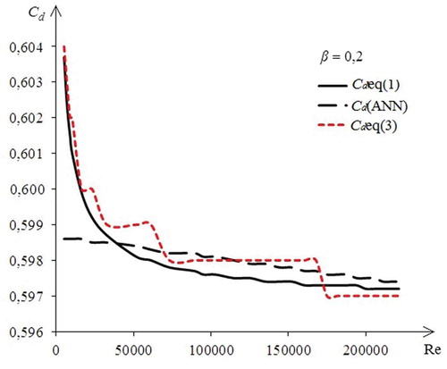
The graphs in Figure 13 show that both methods approximate the original relationship ambiguously. The ANN model of the discharge coefficient is more linear as the Reynolds number increases, as opposed to the fuzzy model of this coefficient. But the fuzzy model of the discharge coefficient, despite its non-linear nature in certain sections of the Reynolds numbers, better repeats the original equation (2)(2) $\begin{array}{rl}& C_d=0,5961+0,0261{\beta }^2-0,216{\beta }^8+0,000521{\left(\frac{{10}^6\beta }{Re}\right)}^{0.7}+\\ & +\left(0,0188+0,0063A\right){\beta }^{3,5}{\left(\frac{{10}^6}{Re}\right)}^{0,3}+\left(0,043+0,08e^{-10L_1}-0,123e^{-7L_1}\right)\times \\ & \times \left(1-0,11A\right)\frac{{\beta }^4}{1-{\beta }^4}-0,031\left(M_2-0,8M_2^{1,1}\right){\beta }^{1,3}+M_3,\end{array}$(2) . A particularly fuzzy model better approximates the original equation on small values of Reynolds numbers, as can be seen from the graph in Figure 13.

Now it is necessary to compare models by considering their relative errors, which can also be calculated using the equation (4)(4) $\delta C_d=\frac{C_{d}eq(2)-C_{d}eq(3)}{C_{d}eq(2)}\cdot 100\mathrm{\%},$(4) . Comparing the graphs in Figure 14, we can conclude that the fuzzy model has higher accuracy over the entire range of Reynolds numbers.

Figure 14. Comparison of relative errors in the discharge coefficient of the present model with two previous models

The work (Dayev 2020) showed that the simulation of the discharge coefficient in the form of an artificial neural network requires a large amount of data that provides reliable calculation of the coefficient values. On the other hand, as it is shown above, fuzzy modeling requires getting more different equations that describe the behavior of this coefficient on different sections of linguistic variables. And as shown above, more fuzzy sets are required for a more accurate approximation of the characteristics, although this work used linear sections on individual fuzzy sets. In the case of neural networks, such problems are excluded, where the accuracy of the models depends on the setting of synaptic weights of neurons.

However, it can be noted that both approaches open up new possibilities for obtaining better and more accurate characteristics of the flow transducers. On the other hand, we can combine both methods and organize neuro-fuzzy models of the discharge coefficient. Perhaps a combination of both methods will produce a model that combines the advantages of both neural networks and fuzzy systems.

Conclusions

Thus, within the framework of this article the problem of realization of characteristics of flow measurement systems by fuzzy sets is solved. The article analyzes the current equation of the discharge coefficient, the structure of the fuzzy system, which plays the role of this coefficient, is proposed. The article provides information about the input fuzzy sets, the construction of a fuzzy rule base in accordance with which the calculation of the discharge coefficient is performed. The graphs of errors between the actual discharge coefficients and their fuzzy analogues depending on Reynolds numbers at different values of diameter ratios are presented. It is established that the magnitude of these errors is very small, which also confirms the prospect of using fuzzy models as separate characteristics of measuring systems of flow rate and quantity. It is shown that for a more accurate approximation of the characteristics, it is necessary to add more fuzzy sets. A comparison of the operation of a fuzzy system with an artificial neural network was performed, which showed the behavior of the error in determining the discharge coefficient. The results obtained are applicable in the case when $\beta =0,2$ and the range of Reynolds numbers is $5000\le Re\le 230000$. The present method is feasible for diameter ratio $0,2\le \beta \le 0,75$ and Reynolds number greater than 5000.

Disclosure statement

No potential conflict of interest was reported by the author(s).

References

- Ahmed, E. N., and A. A. Ghanem. 2020. A novel comprehensive correlation for discharge coefficient of square-edged concentric orifice plate at low Reynolds numbers. Flow Measurement and Instrumentation 73:101751. doi:https://doi.org/10.1016/j.flowmeasinst.2020.101751.
- Baker, O., P. Lau, and K. Tawackolian. 2013. Reynolds number dependence of an orifice plate. Flow Measurement and Instrumentation 30:123–32. doi:https://doi.org/10.1016/j.flowmeasinst.2013.01.009.
- Cristancho, D. E., K. R. Hall, L. A. Coy, and G. A. Iglesias-Silva. 2010. An alternative formulation of the standard orifice equation for natural gas. Flow Measurement and Instrumentation 21 (3):299–301. doi:https://doi.org/10.1016/j.flowmeasinst.2010.03.003.
- Daev, Z. A. 2015. A comparative analysis of the discharge coefficients of variable pressure-drop flowmeters. Measurement Techniques 58 (3):323–26. doi:https://doi.org/10.1007/s11018-015-0708-0.
- Daev, Z. A., and A. K. Kairakbaev. 2017. Measurement of the flow rate of liquids and gases by means of variable pressure drop flow meters with flow straighteners. Measurement Techniques 59 (11):1170–74. doi:https://doi.org/10.1007/s11018-017-1110-x.
- Daev, Z. A. A. 2016. Method for the measurement of a pulsating flow of liquid. Measurement Techniques 59 (3):243–46. doi:https://doi.org/10.1007/s11018-016-0951-z.
- Dayev, Z., A. Kairakbaev, K. Yetilmezsoy, P. Sihag, M. Bahramian, and E. Kıyan. 2021. Approximation of the discharge coefficient of differential pressure flowmeters using different soft computing strategies. Flow Measurement and Instrumentation 79:101913. doi:https://doi.org/10.1016/j.flowmeasinst.2021.101913.
- Dayev, Z. A. 2020. Application of artificial neural networks instead of the orifice plate discharge coefficient. Flow Measurement and Instrumentation 71:101674. doi:https://doi.org/10.1016/j.flowmeasinst.2019.101674.
- Dayev, Z. A., and V. T. Yuluyev. 2019. Invariant system for measuring the flow rate of wet gas on Coriolis flowmeters. Flow Measurement and Instrumentation 70:101653. doi:https://doi.org/10.1016/j.flowmeasinst.2019.101653.
- Farsi, M., H. S. Barjouei, D. A. Wood, H. Ghorbani, N. Mohamadian, S. Davoodi, H. R. Nasriani, and M. A. Alvar. 2021. Prediction of oil flow rate through orifice flow meters: Optimized machine-learning techniques. Measurement 174:108943. doi:https://doi.org/10.1016/j.measurement.2020.108943.
- Gallagher, J. E. 2007. Natural Gas Measurement Handbook, 425. Houston, TX: Gulf Publishing Company.
- ISO 5167–1: 2003. Measurement of fluid flow by means of orifice plates, nozzles and Venturi tubes inserted in circular cross-section conduits running full. 2003. 33.
- Kosko, B. 1994. Fuzzy systems as universal approximators. IEEE Transactions on Computers 43 (11):1329–33. doi:https://doi.org/10.1109/12.324566.
- Kremlevsky, P. P. 2002. Flow meters and counters of substances, 409. Saint Petersburg: Polytechnic.
- LaNasa, P. J., and E. L. Upp. 2014. Fluid Flow Measurement, 296. Oxford: Butterworth-Heinemann.
- Mac, T. T., C. Copot, R. De Keyser, T. D. Tran, and T. Vu. 2016. MIMO fuzzy control for autonomous mobile robot. Journal of Automation and Control Engineering 4 (1):65–70.
- Piegat, A. 2010. Fuzzy Modeling and Control, 728. Heidelberg: Springer-Verlag Berlin and Heidelberg GmbH & Co. KG.
- Pistun, E. P., and L. V. Lesovoi. 2005. Improving the discharge coefficient of the standard orifices of variable pressure-drop flowmeters. Sensors and Systems 6 (5):14–16.
- Postlethwaite, B., and C. Edgar. 2000. A MIMO fuzzy model-based controller. Chemical Engineering Research & Design 78 (4):557–64. doi:https://doi.org/10.1205/026387600527707.
- Reader-Harris, M. 2015. Orifice plates and Venturi tubes, 386. London: Springer International Publishing.
- Reader-Harris, M. J., and J. A. Sattary. 1990. The orifice plate discharge coefficient equation. Flow Measurement and Instrumentation 1 (2):67–76. doi:https://doi.org/10.1016/0955-5986(90)90031-2.
- Reader-Harris, M. J., J. A. Sattary, and E. P. Spearman The orifice plate discharge coefficient equation. East Kilbride, Glasgow: NEL, Progress Report No. PR14: EUEC/17 (EEC005). 1992a.
- Reader-Harris, M. J., J. A. Sattary, and E. P. Spearman The orifice plate discharge coefficient equation, Progress Report No. PR14: EUEC/17 (EEC005), Nat. Eng. Lab. Exec. Agency, East Kilbride, Glasgow. 1992b.
- Reader-Harris, M. J., J. A. Sattary, and E. P. Spearman. 1995. The orifice plate discharge coefficient equation - further work. Flow Measurement and Instrumentation 6 (2):101–14. doi:https://doi.org/10.1016/0955-5986(94)00001-O.
- Reader-Harris, M. J., N. Barton, and D. Hodges. 2012. The effect of contaminated orifice plates on the discharge coefficient. Flow Measurement and Instrumentation 25:2–7. doi:https://doi.org/10.1016/j.flowmeasinst.2011.11.003.
- Stolz, J. 1978. A universal equation for the calculation of discharge coefficient of orifice plates. Flow measurement of fluids (ed. H.H. Dijstelbergen and E.A. Spencer). Amsterdam: North Holland: 519-534.
- Yarushkina, N. G. 2009. Fundamentals of fuzzy and hybrid systems, 320. Moscow: Finance and statistics.