Analysis of Machine Learning Methods for COVID-19 Detection Using Serum Raman Spectroscopy

ABSTRACT

One of the most challenging aspects of the emergent coronavirus disease 2019 (COVID-19) pandemic caused by infection of severe acute respiratory syndrome coronavirus 2 has been the need for massive diagnostic tests to detect and track infection rates at the population level. Current tests such as reverse transcription-polymerase chain reaction can be low-throughput and labor intensive. An ultra-fast and accurate mode of detecting COVID-19 infection is crucial for healthcare workers to make informed decisions in fast-paced clinical settings. The high-dimensional, feature-rich components of Raman spectra and validated predictive power for identifying human disease, cancer, as well as bacterial and viral infections pose the potential to train a supervised classification machine learning algorithm on Raman spectra of patient serum samples to detect COVID-19 infection. We developed a novel stacked subsemble classifier model coupled with an iteratively validated and automated feature selection and engineering workflow to predict COVID-19 infection status from Raman spectra of 250 human serum samples, with a 10-fold cross-validated classification accuracy of 98.0% (98.6% precision and 98.5% recall). Furthermore, we benchmarked nine machine learning and artificial neural network models when evaluated using eight standalone performance metrics to assess whether ensemble methods offered any improvement from baseline machine learning models. Using a rank-normalized scores derived from the performance metrics, the stacked subsemble model ranked higher than the Multi-layer Perceptron, which in turn ranked higher than the eight other machine learning models. This study serves as a proof of concept that stacked ensemble machine learning models are a powerful predictive tool for COVID-19 diagnostics.

Introduction

The coronavirus pandemic (COVID-19) caused by severe acute respiratory syndrome coronavirus 2 (SARS-CoV-2) has evolved into an international public health crisis (Hartley and Perencevich 2020). There exists a tremendous burden on doctors, experts, and material resources needed to massively screen and triage the influx of suspected infected patients (Miller et al. 2020). The early detection of SARS-CoV-2 infection in infected patients is crucial for medical teams to manage patient populations effectively and for policymakers to introduce proactive measures designed to minimize transmission rates.

Diagnostic assays currently used to detect SARS-CoV-2 include reverse transcription quantitative polymerase chain reaction (RT-qPCR) and serological enzyme-linked immunosorbent assay (ELISA). The gold standard RT-qPCR method for developing the diagnostic assays is time-consuming and requires pre-treatment to extract viable RNA from samples (Schmittgen and Livak 2008). Faster RT-qPCR protocols have shown to have technical performance limitations that lead to reduced sensitivity and increased variability (Hilscher 2005). Moreover, the ELISA technique is dependent on the sensitivity of the immunoassay and requires optimal coupling between an enzyme-coupled antibody and abundant viral-specific antigens (Lequin 2005). Raman spectroscopy has recently been proposed as a novel mode of detection of SARS-CoV-2 in vitro (Desai et al. 2020).

Raman spectroscopy involves the irradiation of a sample by a monochromatic light source (Jones et al. 2019). The incident photos undergo inelastic scattering after interacting with the sample, which is measured by the wavelengths of the scattered photons and associated intensities (Jones et al. 2019). The pattern of Raman scatter with characteristic waveform features can be used to quantitatively describe the vibrational motion of molecules in the sample as a unique vibrational fingerprint (Ralbovsky and Lednev 2020). The Raman spectrum is a representation of the intensity of the scatter photon recorded against the Raman shift and often visualized as a spectrum.

The Raman spectroscopy biosensing technique has previously been used to detect hepatitis B virus, dengue virus, and cancer subtypes from human sera samples to a high degree of sensitivity comparable to current diagnostic assay performance (Khan et al. 2018a, 2016; Khan et al. 2018c; Ralbovsky and Lednev 2020). Spectral analyses are often coupled with a range of machine learning models for predictive power, ranging from simple logistic regression models, to advanced multivariate support vector machine and deep learning algorithms (Elias et al. 2004; Gastegger, Behler, and Marquetand 2017; Lussier et al. 2020). More recently, novel transfer learning and deep learning models have been developed to diagnose COVID-19 pneumatic symptoms from chest CT scans (Ko et al. 2020; Silva et al. 2020; Wang et al. 2020). The proven accuracy of state-of-the-art machine learning algorithms for diagnostic assessment poses significant potential and room for improvement for comparable models trained on similarly feature-rich, high-dimensional serum Raman spectra data.

Artificial-intelligence-driven tools can be trained to recognize certain features from the vibrational fingerprint of Raman spectra and predict patient infection status with varying degrees of accuracy, sensitivity, and selectivity. The minimally invasive sample collection for Raman spectroscopy methods in combination with machine learning techniques serves as an potential objective and ultra-fast diagnostic tool in clinical settings (Khan et al. 2018b; Olaetxea et al. 2020; Ralbovsky and Lednev 2020). However, there still remains a debate over the optimal machine learning model to be used with the high-dimensional, highly correlated attributes of Raman spectral data (Lussier et al. 2020). Additionally, the best model for predictive performance in a clinical diagnostic setting is only as good as the metrics that defines its performance. The predictive value of the routinely used accuracy metric to evaluate novel model performance should also be considered alongside sensitivity and specificity metrics as well as in comparison to reference models to holistically evaluate novel algorithms (Handelman et al. 2019; Sharma et al. 2019).

To assess the efficacy of different supervised machine learning algorithms to predict patient infection status using Raman spectral data, we have comparatively benchmarked a broad range of machine learning models trained on the processed Raman scatter spectra of serum samples from COVID-19-infected and healthy patients across eight performance metrics. Furthermore, we have iteratively validated a novel, stacked subsemble binary classifier coupled with a feature selection and engineering pipeline to achieve highly accurate prediction of infection status. Overall, we aim to identify the best-performing machine learning algorithms and develop and optimize an ensemble technique for prediction of patient infection status from Raman spectra as a potential objective, auxiliary tool to make informed clinical decisions during an evolving worldwide pandemic.

Methods

Dataset

This study employed a subset of Raman spectra data of serum samples collected from patients suspected or confirmed to have COVID-19 and serum samples collected from healthy controls (Yin et al. 2020). The raw spectra of the samples were downloaded in preprocessed form before baseline correction and removal of instrumental artifacts. Raman shifts due to undesired noise that manifest in the raw spectrum baseline were normalized by subtracting the mean of the 10 replicates for the Raman intensities of the negative control blank from each sample. Outlier samples of the dataset defined as having wavenumber intensities greater than or less than 3 standard deviations from the mean were excluded from the training and validation dataset. The final set of spectra contained 250 total spectra labeled as part of two patient infection status classes: Healthy (124 samples) and COVID-19 (126 samples).

Wiener Filter

Wiener estimation denoising has been used to calibrate raw Raman spectra from human cells with comparable performance to moving-average filtering and Savitzky—Golay filtering and greater performance on spectra with low signal-to-noise ratio (Bai and Liu 2019). The wiener filter was used to smooth the Raman spectra of samples. Spectra baseline normalization and smoothing before performing PCA reduction has been shown to increase classification accuracy (Ishikawa and Gulick 2013). We suspect that future work will likely show improvements in classification accuracy using spectral data with fine tuned use of denoising filters for baseline correction.

Feature Selection

The decision tree-based ExtraTrees classifier was used for feature selection to extract the top 100 features based on feature importance score. The ExtraTrees classifier was chosen due to its faster speed, greater memory-efficiency, and decreased complexity compared to genetic algorithms for feature selection. The aim of ExtraTrees feature selection is to inform decisions about which features in an input dataset should be trained on to maximize predictive performance and reduce dimensionality by minimizing the number of features selected. The by-product of reduced dimensionality also improves execution time, memory usage, and data efficiency (Handelman et al. 2019). A characteristic feature of decision-tree-based classifiers such as ExtraTrees is that they are able to quantitatively label features with a feature importance score during each split of the forest architecture to quantify the contribution of each feature to the predicted outcome.

Standard Normal Variate Normalization

Standard Normal Variate (SNV) method was used to perform column-wise normalization by subtracting each wavenumber intensity by the mean across all samples and then dividing by the standard deviation across all samples. After SNV, the Raman spectra will be normalized with a mean of 0 and a standard deviation of 1. The normalization makes all spectra comparable in terms of intensities and corrects for systematic errors across samples.

Principal Component Analysis

Principal Component Analysis (PCA) was used to reduce subset of 100 features selected by the ExtraTrees classifier to 26 principal components that captured at least 99% of the total variability of the selected dataset to minimize information loss. This approach creates novel, uncorrelated variables that maximize variance. PCA maintains the predictive performance of machine learning classifiers and minimizes overfitting to complex, noisy patterns often found in high-dimensional data (Howley et al. 2005). The implementation of PCA as a data pre-processing step for common machine learning models trained on high-dimensional, spectral data has shown to improve predictive performance (Howley et al. 2005).

Model Selection

In this study, nine machine learning models were included: Logistic Regression (LR), K Nearest Neighbors (KNN), Support Vector classifier (SV), Decision Tree classifier (DT), Adaboost classifier (AB), Gradient Boost classifier (GB), Random Forest classifier (RF), ExtraTrees classifier (ET), and Multi Layer Perceptron classifier (MLP). The diversity of the nine machine learning models were selected to benchmark their performance to predict patient infection status against a meta-stacked ensemble classifier pipeline based on the following reasons:

1. Eight out of the nine machine learning models were able to model the nonlinear relationship between the predictors (Raman intensity) and output label (patient infection status),

2. Each machine learning model has been thoroughly validated in its use of different forms of independent variables and measurement scales,

3. Each model does not have strict assumptions when trained and validated on high-dimensional Raman spectral data, and

4. A review of the current literature indicated no comprehensive studies that benchmarked a diverse set of machine learning models and a meta-stacked ensemble classifier for assessing patient infection status using Raman spectral data.

The hyperparameters of each baseline machine learning model were exhaustively considered using GridSearchCV or randomly sampled among a number of candidates from a parameter space with a specific distribution using RandomizedSearchCV from the Scikit Learn library (Pedregosa et al. 2011). Benchmark model performance was optimized to achieve a minimum of 90% mean accuracy or greater and comparable results from alternative performance metrics including sensitivity, specificity, and precision. Model parameters are described in Supplementary Information.

Meta-Stacked Subsemble Model

The stacked ensemble model architecture consists of two layers of machine learning models. The first layer of the architecture comprises eight independently trained base machine learning models. The meta model in the second layer uses the predictions of the base models from the first layer as a new training set to make the final class prediction for each sample. The stacking ensemble meta model approach is used since the meta model in the second layer is able to capture the variance and complex patterns from multiple independent base model predictions. Moreover, the meta model may be able to distinguish poor performing base models and compensate by using better performing base models for specific subsets of the data. To optimize the stacked model performance, the eight base models were chosen to be as diverse as possible in their method of class prediction and their hyperparameters were tuned to achieve above 90% 10-fold cross-validated accuracy independently. The meta model was structured as a three-layer perceptron due to its top-in-class performance when parameterized with three hidden layers (50, 30, 10), the ReLU activation function and stochastic gradient descent method with an adaptive learning rate.

When predicting class labels, the Multi-layer Perceptron meta learner in the second, higher-order layer generally performs better when trained on feature-rich class probabilities rather than the predicted class outcome. Thereby, a probabilistic ensemble method was used where base classifiers each returned a matrix composed of the probability that a sample is a member of each class. Thereby, the meta learner is able to consider class probabilities based on the confidence of each base classifier in their prediction and model more nuanced patterns in their prediction rather than only consider class membership outcome as seen in traditional hard-voting ensemble architectures.

Finally, we used an subsemble adaptation of the stacked ensemble architecture first proposed by Sapp et al. to construct the novel ensemble classifier (Sapp, van der Laan, and Canny 2013). Subsembles are based on the idea that localities of feature space have unique properties that are lost when traditional models are trained globally on the entire dataset (Sapp, van der Laan, and Canny 2013). Subsembles partition the feature space and trains base models on each partition, allowing for base models to optimize to local features. The feedforward method used the class probabilities output from the base layer to train the meta model. The meta model is tasked with global generalization across all partitions of the dataset. This technique is particularly powerful when data structures are multi-modal or have characteristic spectral waveform features such as Raman spectra. Subsembles allow base estimators to fit subsets of features to estimate local distributions and facilitates the generalization performance of the meta learner when training on high-dimensional, feature-rich data.

Model Training and Validation

The current configuration of K-fold cross-validation partitioned the dataset into 10 stratified subsets (k = 10), where each subset is made by preserving the percentage of samples for each class. The technique randomly partitions the original input dataset into k equal sized subsamples. Among the k subsamples, one subsample is used as the validation dataset and the remaining subsamples are used as the training dataset. Each partitioned subsample will be used as a validation dataset and the remaining dataset used for model training in successive iterations of the cross-validation procedure. The same train-test procedure will be repeated k times. Each of the nine baseline models and the meta-stacked ensemble model were trained to extract characteristic features associated with one of two classes from the training dataset and predicted the identity of each sample in the validation dataset. This method prevents information leakage from the base models of the meta stacked ensemble model to the meta model for validation of performance metrics. Performance metrics for each iteration of the train-test procedure of K-fold cross-validation were recorded for each baseline machine learning model and the meta-stacked ensemble model were recorded.

Performance Metrics

This study used several measurements to evaluate model performance, including accuracy, precision, recall, F1-Score, area under the Receiving Operating Characteristic (ROC) curve, Cohen’s Kappa, and Matthew’s Correlation (Korotcov et al. 2017).

Model accuracy is a generalized measure of model robustness defined as the percentage of correctly identified class labels out of the total number of samples in the population. Model precision, also termed positive predictive value, is described as the probability that a predicted true label is indeed true. Model recall, also termed true positive rate or sensitivity, is described as the percentage of true class labels correctly identified by the model as true. The F1-score is an aggregate value composed of the harmonic mean of the recall and precision metrics. The subset of metrics composed of accuracy, precision, recall, and F1-score values are bound within the range of 0 and 1, where higher values suggest improved model performance. The ROC curve is visualized by plotting the false positive rate as a function of the recall metric at successive decision thresholds. Decision thresholds are defined as the threshold between 0 and 1 where probability estimates above the threshold will assign a sample to a specific class. The area under the ROC curve measures the ability for the model to distinguish between classes, where 1 indicates perfect classification and 0.5 indicates random classification.

Matthew’s correlation coefficient (MCC) is a measure of model correlation between observed and predicted binary classifications. The MCC metric accounts for true and false positives and negatives and is generally robust to class imbalance (Boughorbel et al. 2017). MCC has values bound within the range of −1 to 1, where −1 indicates total disagreement between observed and predicted labels and 1 indicates perfect agreement between observed and predicted labels. Cohen’s Kappa (CK) is another metric that measures the agreement between two classifiers who each independently classify every sample in the population into mutually exclusive categories (Sim and Wright 2005). The kappa value quantifies the reliability for two independent classifiers, normalized for how often the raters will agree by chance and is bound within the range of 0 to 1. A kappa score of 0 indicates that there is random agreement between classifiers and a kappa score of 1 indicates that there is perfect agreement between classifiers. Time taken for 10-fold cross-validated training and testing on the processed dataset was measured to quantify algorithm time complexity.

Results

Figures 2a and 2b show the mean intensity along with the 95% confidence interval of Raman spectra of serum samples from healthy control patients and COVID-19-infected patients respectively. It is evident that the control serum spectrum showed higher amounts of phenylalanine-containing compounds indicated by more intense peaks at 1001 cm⁻¹ and intense peaks associated with protein components at 1461–1466 cm⁻¹ (González-Solís et al. 2014). Welch’s t-test was performed to determine significant differences between Raman spectra of serum samples as a function of wavenumber. It is evident that there are significant differences in the Raman spectra (p < .05) as a function of time, in particular between 550–650, 1600–1700, and 1800–1970 cm⁻¹. If we examine peak similarity between Figures 1a and 1b, these plots show almost identical peaks at 810 cm⁻¹, 840 cm⁻¹, 1001 cm⁻¹, 1150 cm⁻¹, 1328 cm⁻¹, and 1459 cm⁻¹. The mean healthy spectra at the six peak raman shifts consistently produces Raman intensity at >0.007 a.u. greater than mean COVID-19 spectra.

Figure 1. Two-layer stacking subsemble architecture

Figure 2. a) Mean of the Raman spectra and 95% confidence interval corresponding to serum samples from healthy patient controls (n = 150). b) Mean of the Raman spectra and 95% confidence interval corresponding to serum samples from COVID-19 infected patients (n = 159). c) Features scores by Extra Trees classifier for patient infection status from processed Raman spectra data. d) Boxplots showing the variation in distribution of raman intensities at 810, 842, and 1001 cm⁻¹. t-test statistic and p-value (p < .05) indicated for statistically significant differences between the mean intensity for the COVID-19 group relative to the control group using all spectra

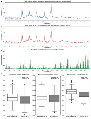
The mean Raman intensity that had the greatest absolute difference at three distinct wavenumbers between healthy control patients and COVID-19-infected patients were visualized as boxplot distributions in Figure 1c). Welch’s t-test showed a statistically significant difference (p < .05) between the means of Raman intensities between the two groups at 810, 842, and 1001 cm⁻¹ and indicates a greater mean intensity in healthy control patients at the selected wavenumbers.

To evaluate the contribution of raman spectral features to the performance of machine learning models, the Extra Trees classifier was used to score features based on their importance score. Figure 1d plots the 10-fold cross-validated relative feature importance score using Extra Trees, where higher scores indicate features that are more likely to positively contribute to accurate classification of Raman spectral data and lower scores indicate poorly contributing features.

Each feature is given a feature importance score and ranked based on this score. Using this metric, we were able to extract the top 100 features as the training dataset for downstream analysis and evaluation of machine learning models. We observed that the wiener filtering and feature selection procedure boosts accuracy of the ensemble classifier by between 3% and 5% compared to when trained on the original pre-processed dataset. Likewise, feature scaling was optimized using standard normal variate scaling following feature selection to produce marked increase in accuracy by 2 土 1.5% 10-fold cross-validated accuracy.

The Raman spectra used as training data for benchmarking machine learning models was processed using PCA to produce 26 principal components from 900 original features that cumulatively captured 99% of the total variance of the original dataset.

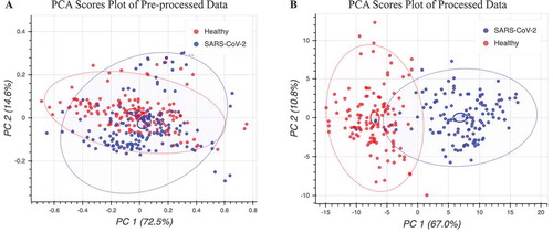
In Figure 3a, the PCA clustering of preprocessed Raman data shows that the separation between the different processed Raman spectra was not linearly separable between the first two principal components. This suggests that additional hyperplanes may exist in higher dimensions beyond two principal components and confirms the feature-rich complexity of the Raman spectral system. The pre-processed data showed that 87.1% of all the spectral variation was accounted for within the first two principal components. The first principal component explained 72.5% of the data variation and the second principal component explained 14.6% of the data variation. Using our feature selection and engineering pipeline to process Raman data, we were able to achieve more clearly defined regions between classes in two principal component dimensions as shown in Figure 3b. The processed data showed that 77.8% of all spectral variation were accounted for within the first two principal components. The first principal component explained 67.0% of the data variation and the second principal component explained 10.8% of the data variation. Comparisons of machine learning model performance using PCA reduction and baseline Raman spectral data yielded consistent improvements of independent model performance using the processed data by 5 土 2.3% 10-fold cross-validated accuracy.

Figure 3. PCA projection of Raman spectra in two dimensions of COVID-19-infected and healthy control patient serum samples. a) PCA visualization of pre-processed Raman spectra, colored according to class. b) PCA visualization of processed Raman spectra using workflow described in methods, colored according to label

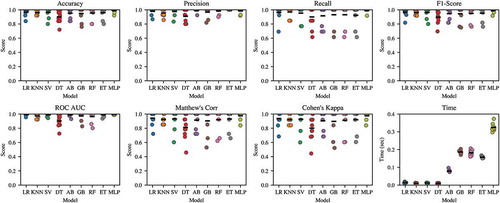
The accuracy, precision, recall, F1-score, area under ROC curve, MCC, CK, and time to train and test baseline models have been summarized in Figure 4. Trained model files are provided in Supplementary Information. We have grouped each performance metric as a standalone stripplot with the mean score indicated for ease of model comparison. Figure 4 shows the scores for each of the 10-folds of the cross-validated train-test procedure grouped by machine learning model. From Figure 4, we see that the cross-validation procedure was successful in introducing variance in the train-test procedure. Base models were likely not overtrained when comparing the consistent predictive performance on training and testing sets. The consistent performance of each baseline model across each performance metric can be indicative of the quality of the models and the generalizability under different testing conditions and data. Nonparametric permutation tests were resampled 1000-fold for each of the nine baseline models and the ensemble model (Golland and Fischl 2003). Each test yielded a statistically significant classification accuracy (p < .05), given the null hypothesis of no difference between a random classifier and tested classifier with an expected mean binary classification accuracy of 50%.

Figure 4. Stripplot for machine learning algorithm performance to classify the test fold when trained on the remaining folds using the 10-fold cross-validation scheme across eight metrics

The ranked normalization approach for aggregate scoring of machine learning model performance across multiple metrics has previously been proposed and was used to rank model performance in Table 1 (Korotcov et al. 2017). The implementation of the ranked normalization approach uses the mean across six performance metrics (MCC, CK, accuracy, precision, recall, and F1-score) to provide an aggregate score to rank the overall performance of each model. The area under the ROC curve was excluded from the ranked normalization approach to ranking models since the stacked subsemble model does not return probabilistic estimates of assigning a sample to a given class needed to produce the area under the ROC curve metric.

Table 1. Ranked normalized scores for each machine learning algorithm by metric (average score over each fold of the 10-fold cross-validation)

Rank	Model	Fit Time	Score Time	MCC	CK	Accuracy	Precision	Recall	F-1 Score	ROC AUC	Ranked Normalized Score
1	Subsemble	16.02	1.04	0.961811	0.959807	0.98	0.985714	0.984615	0.962411		0.972383
2	LR	0.008159	0.006033	0.946427	0.943832	0.972	0.971832	0.976282	0.972806	0.991667	0.963863
3	SV	0.006042	0.00655	0.946843	0.943729	0.972	0.979524	0.967949	0.972063	0.990385	0.963684
4	ET	0.139212	0.032024	0.939377	0.935999	0.968	1	0.937179	0.966576	0.994872	0.957855
5	RF	0.170148	0.027223	0.931685	0.928011	0.964	0.992308	0.937179	0.962576	0.996795	0.952627
6	KNN	0.002107	0.00734	0.924577	0.920126	0.96	0.956593	0.969231	0.96053	0.973077	0.94851
7	MLP	0.362273	0.00638	0.924541	0.920075	0.96	0.992308	0.929487	0.958242	0.986538	0.947442
8	GB	0.204808	0.006385	0.905986	0.903742	0.952	0.954945	0.952564	0.952413	0.987179	0.936942
9	AB	0.069562	0.016664	0.90137	0.896113	0.948	0.976923	0.921795	0.946217	0.992308	0.931736
10	DT	0.003621	0.006375	0.875565	0.871741	0.936	0.925836	0.952564	0.937307	0.935897	0.916502

When models are ranked based on average performance, the Meta-stacked Ensemble Classifier ranked above all nine other baseline machine learning models across the MCC, Accuracy, and Recall performance metrics. The subsemble classifier and the Multi-layer Perceptron classifier produced 98.0% and 96.0% 10-fold cross-validated accuracy. The ensemble classifier produces a mean measurement of 0.930 or greater and a maximal measurement of 1.000 in at least one-fold of the train-test procedure for all metrics except for time. Both the ensemble classifier and Perceptron classifier also consistently achieve above 90% accuracy and similar performance on other metrics except for time regardless of which dataset partition was trained and tested on as part of the 10-fold cross-validation scheme. Time for the 10-fold train-test procedure of the ensemble classifier and the standalone perceptron classifier was 80 seconds and 4 seconds, respectively.

Among the nine baseline models, the Logistic Regression classifier outperforms the other models, including the Multi-layer Perceptron, based on mean CK (0.93569), accuracy (0.972), recall (0.976282), F1-score (0.972806), and the area under the ROC curve (0.991667) metrics.

For MCC, the best performing model was the Support Vector classifier (0.9468843). For precision (positive predictive value), the best performing model was the ExtraTrees classifier (1.000). The Support Vector Classifier and the ExtraTrees classifier both consistently perform among the top three baseline models across five out of seven unique performance metrics. Computationally inexpensive algorithms including Logistic Regression, K-Nearest Neighbors, and to a lesser extent Support Vector Machines and Decision Trees were each able to conduct single train-test procedures on the dataset in under 0.2 seconds. Comparatively, iterative algorithms such as Gradient Boosting, hierarchical tree-based algorithms such as Random Forest and ExtraTrees, and deep learning architectures such as the Multi-layer Perceptron required more time to complete the 10-fold train-test procedure. The Multi-layer Perceptron took the longest time to train and test at over 0.36 seconds, the Gradient Boosting took over 0.20 seconds, and the Extra Trees and Random Forest classifiers took at least 0.13 seconds.

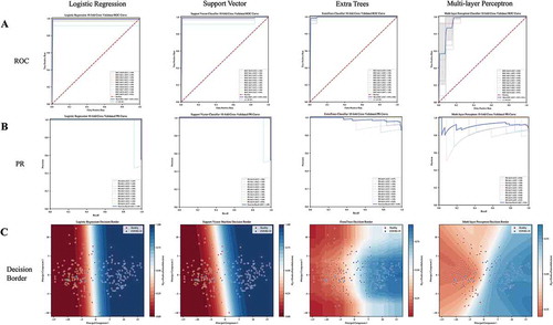
Threshold-free measures such as the ROC and Precision-Recall (PR) curve can give an overview of the performance range across various thresholds (Handelman et al. 2019). With successive thresholds, we are able to produce dynamic scores for support machine learning classifiers. We selected three common machine learning models (Logistic Regression, Linear Support Vector Classifier, and ExtraTrees Classifier) and the Multi-layer Perceptron model to examine the ROC curve, PR curve, and binary classification decision regions in two principal component feature space. In Figure 5a, we observe that the Logistic Regression, Linear Support Vector Classifier, and ExtraTrees Classifier with tuned hyperparameters are able to independently achieve 0.994, 0.990, and 0.989 mean score for the area under the ROC curve metric. A corollary to the ROC curve is the PR curve, which has previously been suggested to give a more informative picture of an algorithm’s performance and whose performance is not strictly related to the same model’s performance using the ROC metric (Davis and Goadrich 2006). Figure 5b shows that each baseline model achieves above 0.98 mean score for the area under the PR curve metric. Comparatively, the Multi-layer Perceptron achieves worse performance with 0.95 and 0.91 mean score for area under the ROC curve and PR curve, respectively. This worse performance is likely due to the need for traditional deep learning algorithms to extract complex features from larger datasets (Najafabadi et al. 2015) and the few samples of the training dataset in this test. The first two principal components of the processed raman spectra are visualized in Figure 5c and decision borders are plotted as contours of predicted class probabilities. We see that the first two principal components of the processed Raman spectra data produce two distinct regions of feature space for each of the two classes. Generally, each of the four selected models were able to distinguish decision regions comprising reasonable class separations and did not overfit to outliers during the cross-validation testing scheme.

Figure 5. a) ROC curve for each fold of the 10-fold cross-validation for the logistic regression, support vector machine, extra trees (extra random forest), and Multi-layer Perceptron machine learning algorithms. b) PR curve for each fold of the 10-fold cross-validation for the logistic regression, support vector machine, extra trees (random forest), and Multi-layer Perceptron machine learning algorithms. c) Decision boundary for the logistic regression, support vector machine, extra trees (random forest), and Multi-layer Perceptron machine learning algorithms in two principal component feature space

To showcase the performance of the stacked subsemble model on each fold, we show the performance of the subsemble model trained and tested using the 10-fold cross-validation scheme across six metrics as shown in Table 2. The stacked subsemble model consistently achieves at least 0.8 or higher in any single fold across each of the six performance metrics. Moreover, the stacked subsemble model consistently produces a score of at least 0.9 or higher for the F1-Score, accuracy, precision, and CK metrics. Conversely, increased variation across different folds used to train the stacked subsemble model for the cross-validation procedure were observed from the MCC and recall metrics. From the results shown in Table 2, the consistent performance throughout each fold of the cross-validation procedure and across multiple unique metrics can serve as a good example of a model that is well balanced.

Table 2. Performance of the stacked subsemble model across six metrics on each of the 10-folds as part of 10-fold cross-validation scheme

	MCC	CK	Accuracy	Precision	Recall	F-1 Score
Fold 1	1	1	1	1	1	1
Fold 2	1	1	0.96	1	1	1
Fold 3	1	1	1	1	1	1
Fold 4	0.849837	0.83871	0.96	1	0.833333	0.909091
Fold 5	1	1	0.96	1	1	0.96
Fold 6	0.9226	0.919614	0.96	0.928571	1	0.962963
Fold 7	1	1	1	1	1	0.96
Fold 8	0.9226	0.919614	1	0.928571	1	0.962963
Fold 9	1	1	1	1	1	1
Fold 10	0.923077	0.920128	0.96	1	0.923077	1
Mean	0.961811	0.959807	0.98	0.985714	0.984615	0.962411

Discussion

To date, Raman spectroscopy remains an exciting field of research with numerous applications due to its complex, feature-rich data that can be processed into machine-readable feature vectors and used to train predictive algorithms. However, the preprocessing steps to transform Raman spectra into machine-readable feature vectors and comparing machine learning, deep learning, and ensemble algorithms that are more capable of extracting these features as valuable trained data to produce predictions on novel data remain a developing area of research. This study aimed to fill the gap in literature by implementing an end-to-end workflow for Raman spectra feature processing, benchmarking several predictive algorithms on the processed dataset, and testing the predictive power of ensemble machine learning methods.

It is worth noting that the appropriate sequence of baseline correction and preprocessing techniques of Raman spectra can cumulatively improve performance by 20–40% (Liu et al. 2017). From our iterative tests that evaluated the use of feature selection, wiener filtering, feature scaling, and PCA reduction at each stage of the preprocessing pipeline compared to baseline data, we were able to cumulatively achieve up to 10% increased accuracy and comparable improvements in precision and recall using the 10-fold cross-validation approach. This result highlights that preprocessing of spectra data is needed to efficiently handle the interference of baseline noise and explicitly retain discriminatory information as intended (Storey and Helmy 2019; Tulsyan et al. 2019). The 3–5% increase in mean accuracy of the ensemble classifier after the use of wiener filtering and feature selection suggests that there are redundant and highly correlated features in the training dataset. Non-essential features can be removed by the ExtraTrees classifier approach to ranking feature importance scores. Likewise, wiener filtering can filter out noise from corrupted signals to provide a smoothed-out estimate of the underlying signal by correcting for outliers. Standard normal variate scaling and PCA reduction further enhances model generalizability by preventing model overfitting and improves the ensemble classifier by up to 5% accuracy. We did not notice obvious effects of class imbalance due to the reasonably balanced class distribution in our processed dataset, but further studies are needed to benchmark the effect of class imbalance often found in real datasets.

From our results, we observed that the stacked ensemble classifier and Multi-layer Perceptron classifier consistently ranked first and second across the seven tested metrics respectively, with the exception of time complexity due to the resource-intensive nature of deep learning algorithms. The K-Nearest Neighbors model consistently ranked higher than even more complex models such as the tree-based Decision Tree and the ensemble Adaboost classifier when evaluating the accuracy, F1-score, area under the ROC curve, MC, and CK metrics. Previous literature has suggested that despite the simplicity of the K-nearest neighbors, this machine learning algorithm remains a frontrunner among other models and is highly scalable in real applications (Deng et al. 2016). In addition, more complex models are prone to overfit and may fail to generalize to novel data (Ying 2019). These superior performance results of the stacked ensemble classifiers and deep neural networks suggest that these algorithms should be further validated under different experimental scenarios of classification using Raman spectra to test for algorithm generalizability on larger, noisier datasets.

Also, the use of several performance metrics to evaluate predictive algorithms sheds new light on model performance under different evaluation scenarios. When evaluating a model’s performance in predicting the positive class, using the area under the PR curve metric is more sensitive to improvements in the positive class (Saito, Rehmsmeier, and Brock 2015). However, if the aim is to evaluate predictive performance of both the positive and negative class and the dataset class distribution is reasonably balanced, then the area under the ROC curve is the more suitable metric (Bradley 1997). Comparatively, the MCC metric is more informative than accuracy and the F1-score in describing binary classification performance since it accounts for the balance ratios between true positives, true negatives, false positives, and false negatives (Chicco and Jurman 2020). Other metrics such as CK and the F1-score require a priori determination of appropriate baseline thresholds and should be constructed based on their relevance in each experimental scenario (Gastegger, Behler, and Marquetand 2017). For example, a random classifier is defined by a CK baseline agreement of 0 in this study and positive CK scores show that the tested classifier performs better than a random classifier (Gastegger, Behler, and Marquetand 2017). The CK metric was shown to more sensitively distinguish performance between machine learning models in this study compared to routinely used accuracy and area under the ROC curve metrics. This means that the optimization of machine learning models using stand-alone or a narrow range of metrics found in most published studies in this field can be misleading. Our approach for comparative benchmarking across a diverse range of models and metrics is one step toward a more well-rounded approach to compare model performance and produce meaningful statistics at a higher level of sensitivity.

There are a few limitations in the current study that we hope to address. First, the study has a potential limitation of a relatively small number of unique samples for each of the two classes in the dataset. Larger datasets are usually needed to improve the robustness of prediction algorithms, especially for data-intensive deep learning models for classification of spectral data (Chen et al. 2014). Second, the binary classification setup of the COVID-19 vs. healthy classification task does not address the continuous spectrum of how COVID-19 infection can manifest in the raman spectra of serum samples across successive timepoints. In the future, we plan to modify our approach by using diverse datasets with labels representative of different stages of infection, such as pre-symptomatic and post-symptomatic stages. Third, we hope to use these temporal features to train a recurrent neural network model due to their ability to extract features of temporal dynamic behavior and conduct comparative benchmarks. At the same time, further optimization of the original model architecture and various feature selection and engineering methods will be tested to improve classification performance further.

Conclusion

In this paper, we propose using a stacked subsemble classifier comprised of a deep learning predictive meta algorithm trained on class probabilities from eight base machine learning models as a classification tool using serum Raman spectra data. We have implemented a workflow for processing Raman spectra data for input into machine learning algorithms, a novel meta-stacked subsemble model for highly accurate supervised classification, and comparative benchmarks between nine baseline machine learning models and the novel subsemble model across eight performance metrics. To test for robustness of the ensemble model and comparatively benchmark the nine base machine learning models, we implemented a 10-fold cross-validation scheme for each of the eight performance metrics on the same dataset. We believe that the pre-processing workflow and evaluation of eight performance metrics across several machine learning models can be applicable to other spectroscopy methods that incorporate machine learning into their predictive algorithms.

Using a combination of our data pre-processing pipeline, as well as fine-tuned base model and meta model hyperparameters of the stacked ensemble classifier, we achieved a maximal accuracy of 100% in one fold and a mean accuracy of 98.0% across all 10 folds in the cross-validation procedure and higher average precision (98.6%) and recall (98.5%) metrics compared to baseline machine learning models and stand-alone deep learning algorithms. Overall, we believe that ensemble machine learning algorithms can be further tuned and scaled as an auxiliary tool for objective clinical diagnosis of COVID-19 cases and support clinical decision-making.

Highlights

• Subsemble achieves 98.4% accuracy on Raman spectra of COVID-19 serum samples.

• Subsemble outperformed nine other machine learning models in several metrics.

• Forest-based feature selection and wiener filtering improved model performance.

Author Statement

All persons who meet authorship criteria are listed as authors, and all authors certify that they have participated sufficiently in the work to take public responsibility for the content, including participation in the concept, design, analysis, writing, or revision of the manuscript. Furthermore, each author certifies that this material or similar material has not been and will not be submitted to or published in any other publication before its appearance in the journal.

Acknowledgements

I would like to thank Colby Banbury for his mentorship as part of the Erevna Research Fellowship.

Disclosure Statement

No potential conflict of interest was reported by the author(s).

Data Availability

The serum Raman spectroscopy data was sourced from Yin et al. (2020) and can be found at 10.6084/m9.figshare.12159924.v1. The computational pipelines for analyzing Raman spectra data, the pre-processing workflow, model performance benchmarks, and saved trained models are available to the public at https://github.com/davidchen0420/Raman_Spectroscopy_COVID_19.

Additional information

Funding

The author received no financial support for the research, authorship, and/or publication of this article.

References

- Bai, Y., and Q. Liu. 2019. Denoising Raman spectra by Wiener estimation with a numerical calibration dataset. Biomedical Optics Express 11 (1):200. doi:https://doi.org/10.1364/boe.11.000200.
- Boughorbel, S., F. Jarray, M. El-Anbari, and Q. Zou. 2017. optimal classifier for imbalanced data using matthews correlation coefficient metric. Edited by Quan Zou. PLOS ONE 12 (6):e0177678. doi:https://doi.org/10.1371/journal.pone.0177678.
- Bradley, A. P. 1997. The use of the area under the ROC curve in the evaluation of machine learning algorithms. Pattern Recognition 30 (7):1145–59. doi:https://doi.org/10.1016/s0031-3203(96)00142-2.
- Chen, Y., Z. Lin, X. Zhao, G. Wang, and Y. Gu. 2014. Deep learning-based classification of hyperspectral data. IEEE Journal of Selected Topics in Applied Earth Observations and Remote Sensing 7 (6):2094–107. doi:https://doi.org/10.1109/jstars.2014.2329330.
- Chicco, D., and G. Jurman. 2020. The advantages of the matthews correlation coefficient (MCC) over F1 score and accuracy in binary classification evaluation. BMC Genomics 21 (1):1. doi:https://doi.org/10.1186/s12864-019-6413-7.
- Davis, J., and M. Goadrich. (2006). The relationship between precision-recall and ROC curves. Proceedings of the 23rd International Conference on Machine Learning - ICML ’06. Pittsburgh, Pennsylvania, USA. doi:https://doi.org/10.1145/1143844.1143874.
- Deng, Z., X. Zhu, D. Cheng, M. Zong, and S. Zhang. 2016. Efficient k NN classification algorithm for big data. Neurocomputing 195:143–48. doi:https://doi.org/10.1016/j.neucom.2015.08.112.
- Desai, S., S. V. Mishra, A. Joshi, D. Sarkar, A. Hole, R. Mishra, M. K. Shilpee Dutt, S. G. Chilakapati, A. Dutt, and A. Dutt. 2020. Raman spectroscopy-based detection of RNA viruses in saliva: A preliminary report. Journal of Biophotonics 13 (10). doi: https://doi.org/10.1002/jbio.202000189.
- Elias, J. E., F. D. Gibbons, O. D. King, F. P. Roth, and S. P. Gygi. 2004. Intensity-based protein identification by machine learning from a library of tandem mass spectra. Nature Biotechnology 22 (2):214–19. doi:https://doi.org/10.1038/nbt930.
- Gastegger, M., J. Behler, and P. Marquetand. 2017. Machine learning molecular dynamics for the simulation of infrared spectra. Chemical Science 8 (10):6924–35. doi:https://doi.org/10.1039/C7SC02267K.
- Golland, P., and B. Fischl. 2003. Permutation tests for classification: Towards statistical significance in image-based studies. In Information processing in medical imaging, ed. C. Taylor and J. Alison Noble, 2732:330–41. Berlin, Heidelberg: Springer Berlin Heidelberg. doi:https://doi.org/10.1007/978-3-540-45087-0_28.
- González-Solís, J. L., J. C. Martínez-Espinosa, L. A. Torres-González, A. Aguilar-Lemarroy, L. F. Jave-Suárez, and P. Palomares-Anda. 2014. Cervical cancer detection based on serum sample Raman spectroscopy. Lasers in Medical Science 29 (3):979–85. doi:https://doi.org/10.1007/s10103-013-1447-6.
- Handelman, G. S., H. K. Kok, R. V. Chandra, A. H. Razavi, S. Huang, M. Brooks, M. J. Lee, and H. Asadi. 2019. Peering into the black box of artificial intelligence: Evaluation metrics of machine learning methods. American Journal of Roentgenology 212 (1):38–43. doi:https://doi.org/10.2214/ajr.18.20224.
- Hartley, D. M., and E. N. Perencevich. 2020. Public Health Interventions for COVID-19: Emerging evidence and Implications for an evolving public health crisis. JAMA 323 (19):1908. doi:https://doi.org/10.1001/jama.2020.5910.
- Hilscher, C. 2005. Faster quantitative real-time PCR protocols may lose sensitivity and show increased variability. Nucleic Acids Research 33 (21):e182–e182. doi:https://doi.org/10.1093/nar/gni181.
- Howley, T., M. G. Madden, M.-L. O’Connell, and A. G. Ryder. 2005. The effect of principal component analysis on machine learning accuracy with high dimensional spectral data. Applications and Innovations in Intelligent Systems XIII:209–22. Accessed January 22, 2021 doi:https://doi.org/10.1007/1-84628-224-1_16
- Ishikawa, S. T., and V. C. Gulick. 2013. An automated mineral classifier using Raman spectra. Computers & Geosciences 54:259–68. doi:https://doi.org/10.1016/j.cageo.2013.01.011.
- Jones, R. R., D. C. Hooper, L. Zhang, D. Wolverson, and V. K. Valev. 2019. Raman techniques: Fundamentals and frontiers. Nanoscale Research Letters 14:1. doi:https://doi.org/10.1186/s11671-019-3039-2.
- Khan, S., R. Ullah, A. Khan, N. Wahab, M. Bilal, and M. Ahmed. 2016. Analysis of dengue infection based on Raman spectroscopy and support vector machine (SVM). Biomedical Optics Express 7 (6):2249. doi:https://doi.org/10.1364/boe.7.002249
- Khan, S., R. Ullah, S. Shahzad, N. Anbreen, M. Bilal, and A. Khan. 2018b. Analysis of tuberculosis disease through Raman spectroscopy and machine learning. Photodiagnosis and Photodynamic Therapy 24 (December):286–91. doi:https://doi.org/10.1016/j.pdpdt.2018.10.014
- Khan, S., R. Ullah, A. Khan, R. Ashraf, H. Ali, M. Bilal, and M. Saleem. 2018a. Analysis of hepatitis B virus infection in blood sera using Raman spectroscopy and machine learning. Photodiagnosis and Photodynamic Therapy 23 (September):89–93. doi:https://doi.org/10.1016/j.pdpdt.2018.05.010.
- Khan, S., R. Ullah, S. Shahzad, S. Javaid, and A. Khan. 2018c. Optical screening of nasopharyngeal cancer using Raman spectroscopy and support vector machine. Optik 157:565–70. doi:https://doi.org/10.1016/j.ijleo.2017.11.097.
- Ko, H., H. Chung, W. S. Kang, K. W. Kim, Y. Shin, S. J. Kang, J. H. Lee, Y. J. Kim, N. Y. Kim, H. Jung, et al. 2020. COVID-19 pneumonia diagnosis using a simple 2D deep learning framework with a single chest CT image: Model development and validation. Journal of Medical Internet Research 22 (6):e19569. doi:https://doi.org/10.2196/19569.
- Korotcov, A., V. Tkachenko, D. P. Russo, and S. Ekins. 2017. Comparison of deep learning with multiple machine learning methods and metrics using diverse drug discovery data sets. Molecular Pharmaceutics 14 (12):4462–75. doi:https://doi.org/10.1021/acs.molpharmaceut.7b00578.
- Lequin, R. M. 2005. Enzyme immunoassay (EIA)/enzyme-linked immunosorbent assay (ELISA). Clinical Chemistry 51 (12):2415–18. doi:https://doi.org/10.1373/clinchem.2005.051532.
- Liu, J., M. Osadchy, L. Ashton, M. Foster, C. J. Solomon, and S. J. Gibson. 2017. Deep convolutional neural networks for raman spectrum recognition: A unified solution. The Analyst 142 (21):4067–74. doi:https://doi.org/10.1039/c7an01371j.
- Lussier, F., V. Thibault, B. Charron, G. Q. Wallace, and J.-F. Masson. 2020. Deep learning and artificial intelligence methods for Raman and surface-enhanced Raman scattering. TrAC Trends in Analytical Chemistry 124 (March):115796. doi:https://doi.org/10.1016/j.trac.2019.115796.
- Miller, I. F., A. D. Becker, B. T. Grenfell, C. Jessica, and E. Metcalf. 2020. Disease and healthcare burden of COVID-19 in the United States. Nature Medicine 26 (8):1212–17. doi:https://doi.org/10.1038/s41591-020-0952-y.
- Najafabadi, M. M., F. Villanustre, T. M. Khoshgoftaar, N. Seliya, R. Wald, and E. Muharemagic. 2015. Deep learning applications and challenges in big data analytics. Journal of Big Data 2 (1):1. doi:https://doi.org/10.1186/s40537-014-0007-7.
- Olaetxea, I., A. Valero, E. Lopez, H. Lafuente, A. Izeta, I. Jaunarena, and A. Seifert. 2020. Machine learning-assisted raman spectroscopy for PH and lactate sensing in body fluids. Analytical Chemistry 92 (20):13888–95. doi:https://doi.org/10.1021/acs.analchem.0c02625.
- Pedregosa, F., G. Varoquaux, A. Gramfort, V. Michel, B. Thirion, O. Grisel, M. Blondel, Prettenhofer, P., Weiss, R., Dubourg, V., Vanderplas, J., Passos, A., Cournapeau, D., Brucher, M., Perrot, M., and D. Duchesnay. 2011. Scikit-learn: Machine learning in Python. The Journal of Machine Learning Research 12 (85):2825−2830.
- Ralbovsky, N. M., and I. K. Lednev. 2020. Towards development of a novel universal medical diagnostic method: Raman spectroscopy and machine learning. Chemical Society Reviews 49 (20):7428–53. doi:https://doi.org/10.1039/D0CS01019G.
- Saito, T., M. Rehmsmeier, and G. Brock. 2015. The precision-recall plot is more informative than the ROC plot when evaluating binary classifiers on imbalanced datasets. Edited by Guy Brock. PLOS ONE 10 (3):e0118432. doi:https://doi.org/10.1371/journal.pone.0118432.
- Sapp, S., M. J. van der Laan, and J. Canny. 2013. Subsemble: An ensemble method for combining subset-specific algorithm fits. Journal of Applied Statistics 41 (6):1247–59. doi:https://doi.org/10.1080/02664763.2013.864263.
- Schmittgen, T. D., and K. J. Livak. 2008. Analyzing real-time PCR data by the comparative CT method. Nature Protocols 3 (6):1101–08. doi:https://doi.org/10.1038/nprot.2008.73.
- Sharma, J., C. Giri, O.-C. Granmo, and M. Goodwin. 2019. Multi-layer intrusion detection system with extratrees feature selection, extreme learning machine ensemble, and softmax aggregation. EURASIP Journal on Information Security 2019 (1). doi: https://doi.org/10.1186/s13635-019-0098-y.
- Silva, P., E. Luz, G. Silva, G. Moreira, R. Silva, D. Lucio, and D. Menotti. 2020. COVID-19 detection in CT images with deep learning: A voting-based scheme and cross-datasets analysis. Informatics in Medicine Unlocked 20:100427. doi:https://doi.org/10.1016/j.imu.2020.100427.
- Sim, J., and C. C. Wright. 2005. The kappa statistic in reliability studies: Use, interpretation, and sample size requirements. Physical Therapy 85 (3):257–68. doi:https://doi.org/10.1093/ptj/85.3.257.
- Storey, E. E., and A. S. Helmy. 2019. Optimized preprocessing and machine learning for quantitative Raman spectroscopy in biology. Journal of Raman Spectroscopy. doi:https://doi.org/10.1002/jrs.5608.
- Tulsyan, A., G. Schorner, H. Khodabandehlou, T. Wang, M. Coufal, and C. Undey. 2019. A machine‐learning approach to calibrate generic raman models for real‐time monitoring of cell culture processes. Biotechnology and Bioengineering 116 (10):2575–86. doi:https://doi.org/10.1002/bit.27100.
- Wang, D., J. Mo, G. Zhou, L. Xu, Y. Liu, and J. Gwak. 2020. An efficient mixture of deep and machine learning models for COVID-19 diagnosis in chest X-ray images. Edited by Jeonghwan Gwak. PLOS ONE 15 (11):e0242535. doi:https://doi.org/10.1371/journal.pone.0242535.
- Ying, X. 2019. An overview of overfitting and its solutions. Journal of Physics. Conference Series 1168:022022. doi:https://doi.org/10.1088/1742-6596/1168/2/022022.
- Yin, G., L. Li, S. Lu, Y. Yin, Y. Su, Y. Zeng, M. Luo, M. Ma, H. Zhou, D. Yao, G. Liu, and J. Lang. 2020. Data and code on serum Raman spectroscopy as an efficient primary screening of coronavirus disease in 2019 (COVID-19). Figshare Dataset. doi:10.6084/m9.figshare.12159924.v1.