Classification of Deep-SAT Images under Label Noise

ABSTRACT

One of the challenges of training artificial intelligence models for classifying satellite images is the presence of label noise in the datasets that are sometimes crowd-source labeled and as a result, somewhat error prone. In our work, we have utilized three labeled satellite image datasets namely, SAT-6, SAT-4, and EuroSAT. The combined dataset consists of over 900,000 image patches that belong to a land cover class. We have applied some standard pixel-based feature extraction algorithms to extract features from the images and then trained those features with various machine learning algorithms. In our experiment, three types of artificial label noises are injected – Noise Completely at Random (NCAR), Noise at Random (NAR) and Noise Not at Random (NNAR) to the training datasets. The noisy data are used to train the algorithms, and the effect of noise on the algorithm performance are compared with noise-free test sets. From our study, the Random Forest and the Back-propagation Neural Network classifiers are found to be the least sensitive to label noises. As label noise is a common scenario in human-labeled image datasets, the current research initiative will help the development of noise robust classification methods for various relevant applications.

Introduction

Now a days, satellite imaging is being used in various fields including crop growth monitoring, rainforest growth time series analysis, urbanization rate monitoring, infrastructural and environmental effect monitoring of calamities like earthquake, forest fire and cyclone or may be even for the estimation of financial capacity of the people of a particular region. But the applications having diverse domains and data interpretation practices are carefully analyzed first to find suitable representation models applicable for a particular scenario. Satellite images used for these applications usually utilize high-resolution images and even for a very small geographical region, the temporal image data can become terra bytes or more in size. Moreover, due to the collection process of satellite images, there is usually a good amount of atmospheric noise present in the images like cloud, aerosol, etc. As a result, the data can be difficult to interpret and label even with the help of an expert labeler. The modern earth orbiting satellites capture images in a wide range of spectrum even outside the visible zone using highly sophisticated sensors. In order to analyze and fully utilize the potential of this huge amount of data in and outside of our visible spectrum, efficient and robust automation technology is a must.

Label noise is a type of noise typically present in the satellite or other crowd-sourced image datasets where a particular training instance is miss-labeled. This usually happens because of human error and inadequate training of the labeler. For example, in the satellite imaging domain, a group of people may be asked to label a particular area for two classes, i.e. roads and houses. Now, as the images are not always clearly distinguishable, a house located very close to a road may be labeled as part of the road by the human labeler. This may happen just randomly or sometimes in the case when the data of different instances look very similar to each other. In the remote-sensing sector, there are thousands of fresh contributors with insufficient training and a scarcity of efficient trainers. For an example, in the agriculture domain, suppose we are training a classifier that distinguishes between green and ready fruits. Now, in the training dataset, entirely labeled by human entity, there will be some instances where a fruit may be just partially ripe. Due to the difference in human judgment, some labelers may categorize that fruit as green while others will categorize the same fruit as ripe. These sorts of labeling errors occur specially in the image datasets very commonly.

The three categories of label noise that we have considered in our study are Noise Completely at Random (NCAR), Noise at Random (NAR) and Noise Not at Random (NNAR). NCAR is the type of noise in labels that is independent of any other variables in the data. It is the scenario where the labeler has made a random mistake. On the other hand, the NAR error model has some dependency to the class labels. Suppose, in a particular application some particular class elements are hard to identify from the satellite image dataset. As a result, that particular class instances will have higher than average probability of being mislabeled. NNAR happens for the boundary class elements. For example, when labeling satellite data using only the RGB (human visible) bands, the difference between trees and light vegetation is comparatively very small. In that case, there can be some labeling error in these instances that is not random but depends on the feature values (RGB values).

Label noise instances disproportionately increase the complexity of machine learning models. For example, in a Decision Tree based classifier, a noisy instance will increase the number of branches in an otherwise perfect leaf node. The effect can be mitigated to some extent using post pruning or other regularization methods based on the algorithm being used. But in general, noisy labels make the classifiers converge slowly, add fluctuations in the model results, and may as well increase the model size and complexity.

Image classification schemes are usually of two types, pixel level and object level. Here NAR and NCAR types of noise are easy to determine but most difficult noise is the NNAR. Interesting thing is that, most of the times, NNAR appears in object-based classifiers (Frank et al. 2017). In pixel-based classification schemes, features can be extracted easily but in object-based classifiers it is more complex than that. In a deep learning network, the features are usually extracted internally by the network and as a result finding and representing the boundary cases are difficult.

In our study, we have injected artificial NCAR, NAR and NNAR noises in three datasets to measure the effect on various machine learning algorithms. We adopted a pixel-based feature extraction scheme for the experiment and injected various levels of noise to measure their effects. The primary objectives of our work are:

1. Measure the effect of different types of label noise on the performance of machine learning based image classification.

2. Analyze the variation of accuracy and model complexity of several machine learning image classification algorithms under the presence of label noise.

3. Report a comparative study of the performance of machine learning models at different percentage of label noise and find the best noise tolerant machine learning model in different noise scenarios.

To the best of our knowledge, the effect of artificial label noise has not been quantitatively measured and compared on satellite image dataset. We believe that our work will help the future researchers develop more noise robust systems for satellite image classification tasks by machine learning models.

Related Works

Frank et al. (2017) discussed the presence of label noise and how it affects image classification on high quality satellite images. The Images for their study were collected from the Christchurch, New Zealand after a massive earthquake attack of February 2011. The images had several rubble features like road, commercial building, green-park, under-construction building and contained red, green and blue band data. There were some confusing pixels to categorize between road and under-construction building types. In their discussion they explained how label noise instances disproportionately increased the complexity of machine learning models. In their experiment, the random forest classifier was found to be the best in a noisy situation and to visualize the accuracy they used the ROC curve with a margin of 0–1. They used the scikit-learn implementation of random forest with 85 trees for implementing the classifier. For Image Segmentation before extracting features the authors used the eCognition software. The eCognition tool is designed for exploring and making better understandable object-based Geospatial data. Basically, in remote sensing industry it helps the extraction of information and change detection in Object-based data.

For label noise injection, they adopted two separate approaches for the pixel based classification and the object based classification schemes. For adding noise in the pixel based classification training data, an x% label noise injection will change the label of x% of the pixels in a training image. For incorporation of label noise in the object based classification, firstly the images are segmented into objects. Then the label of x% objects will be altered to implement an x% noise injection. They injected two types of noise in the training dataset, NAR and NNAR.

After the experimental setup, they took three human labeled training dataset (L1, L2, and L3) which were labeled using three different methodologies and tools to measure the impact of the labeling methods on the classification result. In L1 dataset they applied QGIS Polygon Drawing tools to draw arbitrary polygons. By applying QGIS they found some complexity like imperfect recognition of the rubble. Polygons are better to draw shape in normal area but to specifically identified rubble is not easy. Sometimes image is extremely large and after zooming 10–20 times, just using polygons it is difficult to detect the whole rubble area. For this reason, labeler could have picked non rubble area as damage. Dataset L3 was labeled to detect the areas of rubble. So, the labeler used eCognition segmentation (scale 25) to label that area which he/she think was rubble. For this decision several areas of a sample image were not labeled and many rubble areas were omitted from training set. To address both the issues they developed a web-based image segmentation tool where images were divided into multiple tiles. When a labeler zoom each tile it is also partitioned into several parts by the scale parameter 50. So here a labeler can easily label those areas with rubble because when clicking on a rubble area it automatically glows as red. Dataset L2 was labeled with this tool. In summary L2 dataset was labeled in the best way compared to the L1 and L3 datasets.

The Human-Labeled datasets, L1, L2 and L3 were compared depending on pixel and object-based classifiers. In their study, L1 demonstrated very low performance in prediction of building tops in object-based as well as pixel-based classifiers. L3 in object-based classifier delivered very poor predication than L2 because L3 labeling was the worst. No rubbles predicted by L3 were missed by L2 but several simple rubbles missed by L3 were recognized with L2. But In pixel-based classifier damage classification of L2 was very poor than object-based classifiers.

Pelletier et al. (2017) analyzed the effect of label noise on the performance of classification of land cover mapping of multiple crop types with Support Vector Machine and Random Forest algorithms. Analysis has been done by applying class label, feature label, random and systematic noises to the data. The impact of noise with respect to the number of training classes, input feature vectors, and number of training instances are then analyzed. In their study they used a real dataset and a synthetic dataset. The real dataset consists of Spot-4 and Landsat-8 satellite image data of a particular region in France for the year 2013, which are labeled using the French Land Parcel Information System Database. After some pre-processing on the data to decrease noise, a number of temporal values of different feature vectors were extracted from the dataset. To prepare the synthetic dataset, the learned temporal features for each of the crop types from the real dataset was then used with some Gaussian noise to simulate the weed/vegetation regrowth.

To inject noise in the real dataset, they added some confusion between the summer and winter crops thus tempering the temporal characteristic of the feature vectors. For the synthetic dataset, random noises for each class are selected and added during training. They used two versions of the SVM classifier – one is the linear function and another is the radial basis function (RBF). For multi-class classification, they used the one-vs.-one method. For the Random Forest classifier, they used a maximum allowed tree depth and a minimum allowed threshold value for node split that can help reduce the noise effect significantly. In the model training and evaluation phases, they made ten random 50–50 train-test split with no co-occurrence and later injected different amount of noises to test the model responses.

In their study, it was reported that the label noise of random class was more expensive when the number of training class decreased. From the result, the SVM-RBF classifier obtained the lowest performance. For most part, the SVM-RBF overall performance decreased linearly with higher noise. Random forest and SVM-Linear classifiers showed identical response for up to about 25% noise intensity. For noise above 25%, SVM-Linear was found to be the most robust classifier if not using the multi-spectral features. Through their study, they also showed that the model complexity, computational time and memory requirement increases with the increase in label noise. The systematic noise applied had a more severe effect on the model performances compared to the random noises. Above all, it was showed that with multi-spectral features Random Forest classifier was the most robust one among the three choices.

Land cover data and crop data are the necessary input for agriculture and environment monitoring system. Kussul et al. (2017) proposed a learning model of multilayer deep learning architecture with optical and SAR images. The proposed model reached an accuracy of more than 85%. They applied both unsupervised learning in pre-processing and supervised learning for classification. They collected the dataset from the capital of Ukraine using Sentinal-1A and Landset-8 satellites between dates Oct-2014 to Sep-2015. They collected the time series data of 15 images from Sentinal-1A with 2 combined bands and 4 images in Landest-8 with 6 bands. The data region was 28000 square km and classified with eleven different classes (winter white, bare land, forest, water, winter rapeseed, grassland, spring cereals, soybeans, sunflowers, maize and sugar beet).

The researchers divided their methodology into four segments – pre-processing and segmentation, supervised classification, post-processing and the geospatial analysis. During pre-processing phase the authors used self-organized Kohonen maps (SOMs) for handling missing values and image segmentation. SOMs train in each and every bands separately. The core part of this paper is the supervised classification. In this part the authors took four images with 6 bands from Landsat-8 and 15 images with 2 bands from Sentinal-1A and then made input feature vector size 54 (4*6 + 2*15) for the input of Convolution Neural Network (CNN). The authors used 2 CNN architectures for comparison – 1D CNN with spectral domain and 2D CNN for Spatial domain. They applied the relu activation function which is faster than sigmoid in deep learning. To prevent over-fitting they used L2 regularization with the probability of dropout 0.5 and applied an advanced loss function which is a combination of AdaGrad and RMSprop. In the post-processing and geospatial analysis, they tried to improve result by developing some algorithms and filters. In the result part overall classification accuracy 88.7%, 92.7%, 93.5% and 94.6% were achieved for Random Forest (RF), ENN, 1D and 2D CNN respectively. RF produced less accuracy than Neural Network architectures. Accuracy for water, spring crops, winter rapeseed, and sunflowers were not different from one model to another.

Experimental Method

This section consists of the description of the datasets used in our project, the list of extracted features, and feature analysis, model selection, optimization and tuning methods, as well as the process of artificial label noise incorporation adopted in our study.

The Datasets

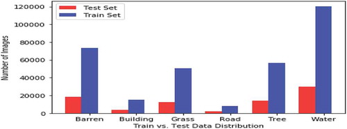
The first dataset used for training and testing in our project is the Deep-Sat image dataset SAT-6 which in turn is built taking images from the National Agriculture Imagery Program (NAIP) satellite image dataset (Basu et al. 2015, 2015). The SAT-6 dataset contains a total of 405,000 labeled images each of size 28 × 28. The images contain four frequency band values, Red, Green, Blue (RGB) and Near Infra-Red (NIR) and they are labeled as six different classes – Building (built up area), Barren Land (empty lands), Tree (forest and large vegetation), Grassland (shrubs), Road and Water. The label file is One-hot encoded. An 80–20 training test distribution is applied to the dataset in the source. As a result there are 324,000 images present in the training set and a total of 81,000 images present in the test set. The ratio of the different class images in the training and test sets are same. Some sample images from the dataset are shown in Figure 1. The total number of images for each class labels in the training and test data sets are presented in Figure 2. The SAT-4 dataset is another Deep-SAT dataset extracted from the same source with 500,000 images belonging to four different classes – barren land, trees, grasslands, and others. Similar to SAT-6, this dataset also has an 80–20 division.

Figure 1. Sample images of various classes from the SAT-6 Dataset

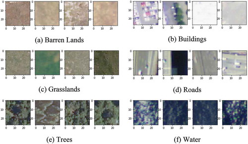
Figure 2. Number of image per class in train and test sets of SAT-6

The EuroSAT dataset, prepared by (Helber, Bischke, and Dengel 2018; Helber et al. 2019) consists 13 band Sentinel-2 images. The 27,000 labeled images are divided into 10 classes and it is also publicly available. The smaller number of images and a higher number of classes present in this dataset gives us the opportunity to analyze and compare the outcome of different algorithms on these datasets.

Feature Value Extraction

A gray level image is a two dimensional array of numbers denoting the intensity levels in various pixel positions. Color images, like RGB images contain pixel intensity levels for three different colors, Red, Green and Blue. Depending on the used dataset, satellite images may have additional intensity values of other frequency spectrums which are not visible to human eye. Table 1 presents a list of different frequency bands collected by the Sentinel-2 earth orbiting satellite.

Table 1. Sentinel-2 imaging bands

Sentinel-2 Bands	Central Wavelength (micro meter)
Band 1 – Coastal Aerosol	0.443
Band 2 – Blue color band	0.490
Band 3 – Green color band	0.560
Band 4 – Red color band	0.665
Band 5 – Vegetation Red Edge	0.705
Band 6 – Vegetation Red Edge	0.740
Band 7 – Vegetation Red Edge	0.783
Band 8 – Near Infra-red (NIR)	0.842
Band 8A – Vegetation Red Edge	0.865
Band 9 – Water vapor	0.945
Band 10 – Short Wave Infrared (SWIR) – Cirrus	1.375
Band 11 – SWIR	1.610
Band 12 – SWIR	2.190

Textual Features

A key part in the image classification task is image feature extraction. Images are a set of 2 dimensional pixel values containing two types of information; one is the intensity information of a single pixel in different frequency channels, and another is the spatial information, that is, the significance of the pixel value relative to other pixel values around it. To extract the spatial information of a particular image, a widely used feature extraction method is Haralick texture features. Haralick (1979) proposed the Haralick features that are widely used to extract image texture information as a set of quantifiable measures.

The suitable texture features to be used for an image dataset may depend on the image type and application domain. Usually image texture means some visual randomness, repeated patterns, and some statistical characteristics. Extracting texture information from an image is important because it gives us an insight of the image (or certain part of an image) as a quantifiable number. As such, the spatial information of the pixel values are preserved here.

At the heart of Haralick texture feature extraction method is the Gray Level Co-occurrence Matrix (GLCM) was proposed by Haralick (1979). In GLCM, firstly a matrix is calculated as in Figure 3 where N is the number of distinct gray level intensity values. The matrix entry at (i, j) cell p (i, j) denotes the number of times intensity level i occurred adjacent to intensity level j in an image. For gray level images, adjacency is calculated for four different directions as in Figures 3 and 4. As a result, if there are N different gray levels used in an image, then we will receive 4 NxN GLCM matrices. From these matrices 14 different statistical texture features are extracted. The features along with the equations to calculate them are explained in Table 2. Although, fourteen features are possible to extract, usually the first 13 of them are used in practice. As a result, for a gray level image, we receive a 13 × 4 matrix of feature values. Usually only the mean of these features in different dimensions is used, so, in practice we receive 13 distinct feature values from a gray level image of any size. For color images, instead of receiving a 13 × 4 matrix, we receive a 13 × 13 matrix. However, as we only keep the mean values of the features in different color and dimensions, so again, we only retain 13 feature values for color images as well.

Table 2. Haralick texture features (Haralick 1979)

Feature Title	Equation
Angular Second Moment	$\sum _i\sum _{j}p\left(i,j\right)$^2
Contrast	$\sum _{n=0}^{{\mathrm{N}}_{\mathrm{g}}-1}{n}^2\{\sum _{i=1}^{{\mathrm{N}}_{\mathrm{g}}}\sum _{j=1}^{{\mathrm{N}}_{\mathrm{g}}}p\left(i,j\right)\},\left|i-j\right|=n$
Correlation	$\frac{{\sum }_i{\sum }_j\left(\mathrm{i}\mathrm{j}\right)\mathrm{p}\left(\mathrm{i},\mathrm{j}\right)-{\mu }_{\chi }{\mu }_{\gamma }}{{\sigma }_{\chi }{\sigma }_{\gamma }}$$Where{\mu }_{\chi },{\mu }_{\gamma },{\sigma }_{\chi }\mathrm{a}\mathrm{n}\mathrm{d}{\sigma }_{\gamma }arethemeansandstd.$$deviationsf{p}_{\chi }and{p}_{\gamma },thepartialprobability$$densityfunctions$
Sum of Squares: Variance	$\sum _i\sum _j{\left(i-\mu \right)}^{2}p\left(i,j\right)$
Invers Difference Moment	$\sum _i\sum _j\frac{1}{1+{\left(i-j\right)}^2}p\left(j,j\right)$
Sum Average	$\sum _{i=2}^{2N_g}i{\mathrm{p}}_{\chi +\gamma }\left(i\right)$where x and y are the coordinates of anentry in the co-occurrenece matrix, and pχ+γ(i) is the probability of occurrence matrix coordinates summing to x+y
Sum Variance	$\sum _{i=2}^{2N_g}{\left(i-f_8\right)}^2{{\mathrm{p}}_{\chi +}}_{\gamma }\left(i\right)$
Sum Entropy	$-\sum _{i=2}^{2N_g}{p_x}_{+\gamma }\left(i\right)log\left\{{{\mathrm{p}}_{\mathrm{x}}}_{+\gamma }\left(i\right)\right\}=f_8$
Entropy	$-\sum _i\sum _{j}p\left(i,j\right)\mathrm{l}\mathrm{o}\mathrm{g}(p\left(i,j\right)$
Difference Variance	$\sum _{i=o}^{N_g-1}{i}^2{\mathrm{p}}_{\chi -\gamma }\left(i\right)$
Difference entropy	$-\sum _{i=o}^{N_g-1}{\mathrm{p}}_{\chi }-{\mathrm{p}}_{\gamma }\left(i\right)\mathrm{l}\mathrm{o}\mathrm{g}\left\{{\mathrm{p}}_{\chi -\gamma }\left(i\right)\right\}$
Info. Measure of Correlation 1	$\frac{HXY-HXY1}{\mathrm{m}\mathrm{a}\mathrm{x}\left\{HX,Hy\right\}}$
Info. Measure of Correlation 2	${\left(1-\mathrm{e}\mathrm{x}\mathrm{p}\left[-2\left(\mathrm{H}\mathrm{X}\mathrm{Y}2-\mathrm{H}\mathrm{X}\mathrm{Y}\right)\right]\right)}^{\frac{1}{2}}$ $whereHXY=-\sum _i\sum _{j}p\left(i,j\right)\mathrm{l}\mathrm{o}\mathrm{g}(p\left(i,j\right),HX,$ $HYaretheentropiesofpxandpy,HXY1=$$-\sum _i\sum _{j}p\left(i,j\right)log\left\{{\mathrm{p}}_{\chi }\left(\mathrm{i}\right){\mathrm{p}}_{\gamma }\left(j\right)\right\}$ HXY2 = $-\sum _i\sum _j{p}_{\chi }\left(\mathrm{i}\right){\mathrm{p}}_{\gamma }\left(\mathrm{j}\right)\mathrm{l}\mathrm{o}\mathrm{g}\left\{{\mathrm{p}}_{\chi }\left(\mathrm{i}\right){\mathrm{p}}_{\gamma }\left(\mathrm{j}\right)\right\}$
Max. Correlation Coefficient	$SquarerootofthesecondlargesteigenvalueofQ$Where $Q\left(i,j\right)=\sum _k\frac{p\left(i,k\right)p\left(j,k\right)}{{\mathrm{p}}_{\chi }\left(\mathrm{i}\right){\mathrm{p}}_{\gamma }\left(k\right)}$

Figure 3. GLCM matrix for N color levels

Figure 4. Four directions for GLCM adjacency calculation

In our initial model development, we have used all these 13 features for training and testing. For the Haralick feature extraction process, we have used the Mahotas implementation of Python (Coelho 2013).

HSV Color Features

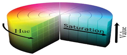
The next three features we have used in our study are the mean HSV color values (HSV 2021) of the images. The HSV color representation system is explained in Figure 5 as a color wheel. The Hue value denotes a particular color in the wheel while the Saturation determines the amount of white color mixed with the Hue selected color. Value determines the brightness, which is how much black color is mixed with the color. In many image processing and computer vision tasks the HSV color features are used instead of their RGB counterpart because, in an RGB image, the color values and the intensity (luminance) values both depend on the Red, Green and Blue values. As a result, in the RGB color space, the color values are being divided into three dimension and along with it, the intensity and saturation of the color is also spreading. But in the HSV model, the H, S, and V values are all independent and can be used as separate unrelated feature dimensions for easier model training.

Figure 5. HSV color wheel (HSV 2021)

Normalized Difference Vegetation Index (NDVI)

NDVI is used for monitoring live green vegetation from satellite imaging data. It incorporates the near infra-red band (NIR) in feature extraction. Leaves and plantations with chlorophyll usually absorbs sunlight from the visible spectrum (below 0.7 micro meters). However, they reflects the NIR band spectrum and appears bright in that region. As a result, the NDVI value is about 1 for the leaves and other biomass canopies. NDVI values are sensitive to soil and atmosphere effects though. As a result, in our study we have used some other extra features all of which incorporate the NIR band data as well.

(1) $\mathrm{N}\mathrm{D}\mathrm{V}\mathrm{I}=\left(\mathrm{N}\mathrm{I}\mathrm{R}-\mathrm{R}\mathrm{e}\mathrm{d}\right)/\left(\mathrm{N}\mathrm{I}\mathrm{R}+\mathrm{R}\mathrm{e}\mathrm{d}\right)$(1)

Atmospherically Resistant Vegetation Index (ARVI)

ARVI is resistant to the air pollution such as dust and smoke. As a result, it is more suitable to monitor vegetation near big city or metropolitan areas.

(2) $\mathrm{A}\mathrm{R}\mathrm{V}\mathrm{I}=\left(\mathrm{N}\mathrm{I}\mathrm{R}-\left(2\ast \mathrm{R}\mathrm{e}\mathrm{d}\right)+\mathrm{B}\mathrm{l}\mathrm{u}\mathrm{e}\right)/\left(\mathrm{N}\mathrm{I}\mathrm{R}+\left(2\ast \mathrm{R}\mathrm{e}\mathrm{d}\right)+\mathrm{B}\mathrm{l}\mathrm{u}\mathrm{e}\right)$(2)

Enhanced Vegetation Index (EVI)

EVI proposed by Huete et al. (1997) is used to correct both the atmospheric and soil background effect on vegetation index measurement. EVI is more suitable to monitor the vegetation of rainforest regions. There are two variations of EVI, EVI-1 and EVI-2 (Jiang et al. 2007). We have used both of them in our primary feature space. In EVI 2, the Blue color band is not used in the equation. The authors have proposed that by not using an extra band (blue) it makes the equation less sensitive toward satellite sensor equipment and hence, make it more robust.

(3) $\mathrm{E}\mathrm{V}\mathrm{I}1=2.5\ast \left(\left(\mathrm{N}\mathrm{I}\mathrm{R}-\mathrm{R}\mathrm{e}\mathrm{d}\right)/\left(\left(\mathrm{N}\mathrm{I}\mathrm{R}\right)+\left(6\ast \mathrm{R}\mathrm{e}\mathrm{d}\right)-\left(7.5\ast \mathrm{B}\mathrm{l}\mathrm{u}\mathrm{e}\right)+1\right)\right)$(3)

(4) $\mathrm{E}\mathrm{V}\mathrm{I}2=2.5\ast \left(\mathrm{N}\mathrm{I}\mathrm{R}-\mathrm{R}\mathrm{E}\mathrm{D}\right)/\left(\mathrm{N}\mathrm{I}\mathrm{R}+2.4\ast \mathrm{R}\mathrm{E}\mathrm{D}+1.0\right)$(4)

In our study, we have used 13 Haralick texture features, 3 HSV features, one for each of NDVI, ARVI, EVI1 and EVI2; a total of 20 features. Note that, all the feature values are transformed using the ‘StandardScaler’ method of the scikit-learn library before using them for training. It is important for many machine learning algorithms that the data is transformed to have 0 mean and unit standard deviation. The StandardScaler method does it for our datasets. After standardization, we have trained a few machine learning algorithms with limited dataset size and tested the results. At this point, we have run Linear Discriminant Analysis to analyze the feature importance. In the subsequent subsections, these processes are described in details.

Machine Learning Algorithms

Random Forest (RF) Based Classification

A random forest classifier consists of many independent decision trees (Breiman. 2001). Each of these decision trees gives a class as output for a particular test case. The final result is the class label selected by most of the trees. As there is no such correlation among those independent models the result is very accurate and noise robust. In our implementation, at first, we train a RF with 100 trees using 50,000 training images from the SAT-6 dataset and test the accuracy on 10,000 images. The classifier returns 99.28% accuracy on the test data. Using this result, we calculate the feature importance for the currently used 20 features. The result is given in the Figure 6. As it can be seen from the figure, some of features are really significant while some are not that much. We next verify the result with a limited training and test case for the rest of the Machine Learning algorithms.

Figure 6. Feature importance analysis using random forest classifier on SAT-6

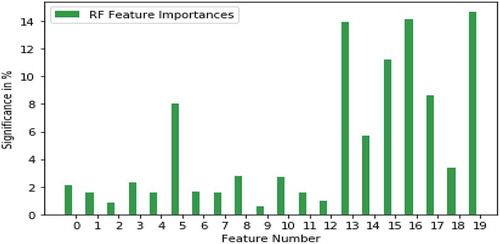
Our Random Forest classifier had 100 Decision Trees with ‘min_samples_leaf’ parameter value set to 2. The ‘min_samples_leaf’ in the scikit-learn implementation, when set to 2, for the random forest implementation will require a leaf to be split only if all the resulting leaves contain at least 2 training instances after the split. This will apply some pre-pruning to the resulting trees and as a result will make the classifier more noise robust.

Support Vector Classifier (SVC)

SVC separates classes by generating a hyper-plane. To separate the data linearly, they are embedded into higher dimensions if needed. Depending on the classification scenario it can use different kernel functions like Linear, or Radial Basis function. In SVC implementation, there are some parameters that can be adjusted to get better result out of it. A typical Support Vector Classifier implementation can usually classify between two different classes only using a single hyper-plane. In our dataset however, there are six different classes. In order to achieve multi class classification using Support Vector Machines, there are two ways in scikit-learn – the one-vs-one and the one-vs-many classifiers. In the one-vs-one classifier, a separate SVC is trained for each of the ^NC₂ choice of class labels. This is time consuming and the one-vs-many classifier is usually preferable. Once a test instance is received, the classifier that successfully classify the instance positively with highest confidence value will be selected.

In our experiment, the Support Vector Classifier we used had L2 regularization. We experimented with the strength of the regularization parameter C to diminish the effect of label noise on the classifier performance, but it still could not provide satisfactory result. The kernel we used was Radial Basis function with Gamma set to the default value of 1/ (number of features * Training set variance). The maximum iteration was set to 50 with a 5-fold cross validation during training.

Logistic Regression Classifier

This is a very simple way to solve classification problems. It classifies inputs using an activation function like sigmoid. For a two-class problem, Binary Logistic Regression is used typically. For our multiclass problem, the one-vs-rest (OVR) method is applied. In Logistic Regression classify inputs a threshold value of output is selected. If the output of the activation function is less than the threshold value, then it will be classified as one class if not then it will be classified as the other class. In our experiment, with 50,000 SAT-6 training data, the accuracy of Logistic Regression (OVR) algorithm is 97.06% for 20 features. In our experiment, we used the default L2 regularization with C = 1 and maximum iteration = 100 for training the classifier.

Neural Network Based Classifier

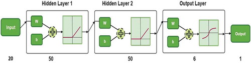
The last classifier that we have used for our study is a fully connected Neural Network with 2 hidden layers having 50 fully connected neurons each and an output softmax layer. The hidden layers had 20% drop ratio and the ‘relu’ function as the activation function. During training Batch Normalization was applied with batch size = 500. 15% of the training data in each epoch was left aside for model validation. The maximum number of epoch was set to be 100. With 50,000 training data and 20 feature values, the training stops at 86th epoch with 99.02% accuracy. The training continues till the bounded 100 epoch but the accuracy increases to be 99.04%. An overview of the network is provided in Figure 7.

Figure 7. Overview of the Neural Network classifier (SAT-6)

Artificial Label Noise Injection

In our study, we have worked with NCAR, NAR and NNAR label noises. For a varying amount of label noise, we have measured the response of the learning time, efficiency and model sizes.

Noise Completely at Random (NCAR)

In order to incorporate the NCAR noise in the train data we randomly picked up to 20% training samples and altered their label to a random different label. For each of these tempered training sets, we retrained the machine learning models to compare the change in different performance measures. As expected, the noise affected our model accuracies, convergence time and model size. But the effect severity was different for different algorithms.

Noise at Random (NAR)

For injecting the NAR noise, we individually picked the different classes one at a time, and altered up to 20% of the training instances belonging to that class. All other training cases remained untouched. After the noisy data was trained with the machine learning models, the results were stored for analysis.

Noise Not at Random (NNAR)

The NNAR noise model in our study is implemented using the Nearest Neighbor approach similar to Garcia et al. (2018). Due to the high memory and processing time requirement, we have utilized only the EuroSAT dataset for this part of the analysis. The experiment is conducted by first calculating the nearest neighbor points for all the multi-dimensional image pixel values of same and different class. Then, the ratio of these two distances are calculated as an indicator to detect the boundary class instances using Equation (5)(5) $DistanceRatio=\frac{\mathrm{M}\mathrm{i}\mathrm{n}\mathrm{i}\mathrm{m}\mathrm{u}\mathrm{m}\mathrm{I}\mathrm{n}\mathrm{t}\mathrm{e}\mathrm{r}\mathrm{C}\mathrm{l}\mathrm{a}\mathrm{s}\mathrm{s}\mathrm{N}\mathrm{e}\mathrm{i}\mathrm{g}\mathrm{h}\mathrm{b}\mathrm{o}\mathrm{u}\mathrm{r}\mathrm{D}\mathrm{i}\mathrm{s}\mathrm{t}\mathrm{a}\mathrm{n}\mathrm{c}\mathrm{e}}{\mathrm{M}\mathrm{i}\mathrm{n}\mathrm{i}\mathrm{m}\mathrm{u}\mathrm{m}\mathrm{I}\mathrm{n}\mathrm{t}\mathrm{r}\mathrm{a}\mathrm{C}\mathrm{l}\mathrm{a}\mathrm{s}\mathrm{s}\mathrm{N}\mathrm{e}\mathrm{i}\mathrm{g}\mathrm{h}\mathrm{b}\mathrm{o}\mathrm{u}\mathrm{r}\mathrm{D}\mathrm{i}\mathrm{s}\mathrm{t}\mathrm{a}\mathrm{n}\mathrm{c}\mathrm{e}}$(5) . Now, when injecting label noise, these boundary class instances, sorted in the ascending order of the Distance Ratio are targeted and their labels are altered. The difference of our approach from the Nearest Neighbor approach proposed by Garcia et al. in (Garcia et al. 2018) is that, when assigning an alternate noisy label to a point, we assigned the label of the same nearest inter class neighbor that was previously used for the calculation of the Distance Ratio in Equation (5)(5) $DistanceRatio=\frac{\mathrm{M}\mathrm{i}\mathrm{n}\mathrm{i}\mathrm{m}\mathrm{u}\mathrm{m}\mathrm{I}\mathrm{n}\mathrm{t}\mathrm{e}\mathrm{r}\mathrm{C}\mathrm{l}\mathrm{a}\mathrm{s}\mathrm{s}\mathrm{N}\mathrm{e}\mathrm{i}\mathrm{g}\mathrm{h}\mathrm{b}\mathrm{o}\mathrm{u}\mathrm{r}\mathrm{D}\mathrm{i}\mathrm{s}\mathrm{t}\mathrm{a}\mathrm{n}\mathrm{c}\mathrm{e}}{\mathrm{M}\mathrm{i}\mathrm{n}\mathrm{i}\mathrm{m}\mathrm{u}\mathrm{m}\mathrm{I}\mathrm{n}\mathrm{t}\mathrm{r}\mathrm{a}\mathrm{C}\mathrm{l}\mathrm{a}\mathrm{s}\mathrm{s}\mathrm{N}\mathrm{e}\mathrm{i}\mathrm{g}\mathrm{h}\mathrm{b}\mathrm{o}\mathrm{u}\mathrm{r}\mathrm{D}\mathrm{i}\mathrm{s}\mathrm{t}\mathrm{a}\mathrm{n}\mathrm{c}\mathrm{e}}$(5) . This way, the noise is reflects an error that would be done by a human labeler with higher probability.

(5) $DistanceRatio=\frac{\mathrm{M}\mathrm{i}\mathrm{n}\mathrm{i}\mathrm{m}\mathrm{u}\mathrm{m}\mathrm{I}\mathrm{n}\mathrm{t}\mathrm{e}\mathrm{r}\mathrm{C}\mathrm{l}\mathrm{a}\mathrm{s}\mathrm{s}\mathrm{N}\mathrm{e}\mathrm{i}\mathrm{g}\mathrm{h}\mathrm{b}\mathrm{o}\mathrm{u}\mathrm{r}\mathrm{D}\mathrm{i}\mathrm{s}\mathrm{t}\mathrm{a}\mathrm{n}\mathrm{c}\mathrm{e}}{\mathrm{M}\mathrm{i}\mathrm{n}\mathrm{i}\mathrm{m}\mathrm{u}\mathrm{m}\mathrm{I}\mathrm{n}\mathrm{t}\mathrm{r}\mathrm{a}\mathrm{C}\mathrm{l}\mathrm{a}\mathrm{s}\mathrm{s}\mathrm{N}\mathrm{e}\mathrm{i}\mathrm{g}\mathrm{h}\mathrm{b}\mathrm{o}\mathrm{u}\mathrm{r}\mathrm{D}\mathrm{i}\mathrm{s}\mathrm{t}\mathrm{a}\mathrm{n}\mathrm{c}\mathrm{e}}$(5)

Result Analysis

Model Comparison with Clean Labels

In the absence of any label noise, all the machine learning algorithms showed very good accuracy, except for the Support Vector Classifier (SVC). Although other algorithms showed 97–99% accuracy on the test data, the highest accuracy of the SVC was 85% for the SAT-6 dataset. A comparative performance of the models in the absence of noise is shown in Tables 3 and 4. From the result, the Random Forest and the Neural Network models are found to be the best in terms of accuracy, followed by Logistic Regression. Moreover, the Logistic Regression algorithm is very fast to train and training the Neural Network model is found to be the slowest.

Table 3. Test accuracy of the algorithms in the absence of noise

Algorithm	Accuracy (SAT-6)	Accuracy (SAT-4)	Accuracy (EuroSAT)
Neural Network	99.30	99.22	97.24
Random Forest	99.64	99.62	98.24
Logistic Regression	97.05	92.17	84.31
Support Vector Classifier	85.80	55.44	65.37

Table 4. Algorithm training time in the absence of noise

Algorithm	Training Time (s) (SAT-6)	Training Time (s) (SAT-4)	Training Time (s) (EuroSAT)
Neural Network	251	214.87	22.74
Random Forest	84	186	7.66
Logistic Regression	46.9	18.09	4.61
Support Vector Classifier	197	127.33	1.95

Analysis with NCAR Label Noise

Accuracy Analysis

In the presence of up to 20% NCAR label noise, the most robust classification algorithm was found to be the Random Forest Classifier (Figure 8). The test accuracy of the algorithm was a consistent 99.60% to 99.67% on the SAT-6 dataset, 99.44% to 99.65% on the SAT-4 dataset and 97.78% to 98.41% on the EuroSAT dataset with a mean accuracy of 98.94% to 99.24%. The accuracy of the Neural Network algorithm under various degree of NCAR label noise is quite to that as well. In addition to that, the network size of a neural network model is fixed irrespective of the ratio of label noise present in the dataset. This noise independence makes it attractive to certain implementations where model size is a concern. The Logistic Regression Classifier used in our experiment showed a slight decrease in accuracy when faced with up to 20% NCAR label noise (from 90.89% to 88.31%).

Figure 8. Mean accuracy of the algorithms under NCAR label noise

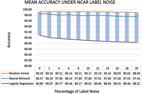
The Support Vector Classifier used in our experiment showed very high sensitivity to NCAR noise. Even a 2% noise set the test accuracy off to about 15%. With more regularization (C = 0.2) the model showed some performance improvement (around 25% accuracy) but it was also taking a high amount of time to converge. As such, we did not further investigate the algorithm for higher noise percentage.

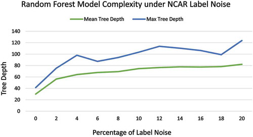
Model Complexity Analysis

One key effect of training data label noise is its effect on the model complexity or training time. In respect of accuracy, the Random Forest algorithm showed the best result under NCAR label noise. However, the maximum and average depths of the decision trees inside the random forests were getting considerably larger in the presence of noise. As such, the training time requirement was also increasing with noise during our experiment. A comparison of mean depth of the random forest trees and maximum tree depth with respect to various amount of NCAR label noise percentage are shown in Figure 9.

Figure 9. Mean and max depth of the random forest trees under NCAR noise

For the Neural Network models, once the training is completed, the model size is always fixed and irrespective of the dataset properties. However, the number of epochs required for the network to converge can vary depending on label noise. However, in our experiment with moderate label noise (up to 20%) the training process proceeded uniformly. As such we did not find any significant deviation in neural network model training complexity which could be attributed to the presence of label noise.

Logistic Regression classifier models were much faster to train compared to the Random Forest and Neural Network models. Complexity wise, they did not show too much sensitivity to the presence of label noise as well.

Analysis with NAR Label Noise

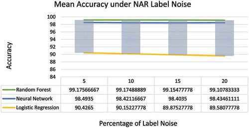
The NAR noise model in our study is evaluated by injecting up to 20% label noise to different class labels and comparing the effect on mean accuracies and other model parameters. By taking average of the resulting values for different percentage of noise, we have compared the individual algorithms’ performance under the NAR label noise.

The effect of NAR noise on the three classifiers is presented in Figure 10. It is seen from the figure that the mean accuracies of the three algorithms exposed to various degree of NAR label noises were pretty stable.

Figure 10. Effect of NAR noise on the three algorithms

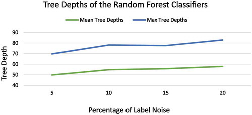
As in the case of NCAR noise, the mean and max tree depths of the RF classifiers gradually increase under NAR noise (Figure 11). However, the noise have not affected the training time or model convergence time for the Neural Network and Logistic Regression classifiers.

Figure 11. Effect of NAR noise on the Random Forest Classifier complexity

Model Analysis with NNAR Label Noise

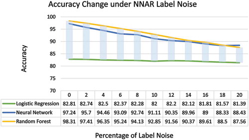
In our study, the NNAR noise applied on the EuroSAT dataset training labels exhibits a stronger effect on the machine learning models in comparison to the previous two noise models (Figure 12). The Random Forest model, in presence of 20% NNAR noise is showing only 87.56% accuracy while it was 98.15% for 20% NAR noise and 97.78% under for 20% NCAR noise. The neural net model is also showing almost a similar result. However, it is understandable because the NNAR noise is applied on the boundary instances.

Figure 12. Effect of NNAR noise on the classification algorithms

Discussion

The results of our experiments indicate that Random Forest is the preferred classifier under small to moderate level of label noise where accuracy is the primary concern. However, as the forest tree sizes grow quite rapidly with the increase of noise, and we know that the size of a decision tree increases exponentially along with its depth, implementing Random Forest models in a limited memory scenario could be a concern.

The Back-propagation Neural Network is found almost as good as the Random Forest classifier with the added advantage of a minute and fixed model size; which makes it suitable where memory limit is a concern. One vs. Rest (OVR) Logistic Regression is found to have lower accuracy compared to Random Forest and Neural Network. On the upside though, the Logistic Regression models took relatively less time to train and hence, can be suitable for some limited processing power environments such as online learning.

It is found that the NNAR type of noise negatively affected the training accuracy the most. In our noise injection process for NNAR, we specifically changed the labels of the boundary instances (pre-selected) to the closest alternate class labels which made the model generalization most difficult.

Conclusion

In this study, varying degree of artificial label noise (NCAR, NAR and NNAR noise models) is applied on three labeled satellite image datasets. The effect of this label noise on three machine learning based Image Classification algorithms (Back-propagation Neural Network, Random Forest and Logistic Regression) are then assessed. The step by step incremental noise injection and comparison method applied in our study can be applied to other datasets and fields of study where there is a high probability of label noise present on the data and different artificial intelligence techniques are used to train on those data.

As a future work, we want to experiment the effect of label noise on various model regularization methods. We also want to explore other forms of label noises and analyze algorithm performances. In this study we utilized a fixed set of handpicked features. In the future we want to use CNN based automatic feature extraction methods, and assess the model performances in both noisy and noiseless scenarios.

Acknowledgments

The authors sincerely thank the anonymous reviewers and the editor-in-chief of Applied Artificial Intelligence for their valuable, insightful comments, suggestions and reviews that improve the quality of the article.

Disclosure statement

No potential conflict of interest was reported by the author(s).

Data Availability Statement

All the datasets used in this study are used and make publicly available in (Basu et al. 2015, 2015; Helber, Bischke, and Dengel 2018; Helber et al. 2019).

Correction Statement

This article has been republished with minor changes. These changes do not impact the academic content of the article.

Additional information

Funding

This work is supported by Faculty Research Grant [CTRG-20-SEPS-14], North South University, Bashundhara, Dhaka 1229, Bangladesh. The authors sincerely thank the anonymous reviewers and the editor-in-chief of Applied Artificial Intelligence for their valuable, insightful comments, suggestions and reviews that improve the quality of the article.

References

- Basu, S., S. Ganguly, S. Mukhopadhyay, R. Dibiano, M. Karki, and R. Nemani. 2015. DeepSat - A learning framework for satellite imagery. ACM SIGSPATIAL 2015: Proceedings of the 23rd SIGSPATIAL International Conference on Advances in Geographic Information Systems. Seattle, Washington, United States. November 2015 Article No.: 37. 1–10. doi:https://doi.org/10.1145/2820783.2820816
- Breiman. 2001. Random Forests. Machine Learning 45(1):5–32. doi:https://doi.org/10.1023/A:1010933404324.
- Coelho, L. P. 2013. Mahotas: Open source software for scriptable computer vision. Journal of Open Research Software 1 (1):e3. doi:https://doi.org/10.5334/jors.ac.
- Frank, J., U. Rebbapragada, J. Bialas, T. Oommen, and T. C. Havens. 2017. Effect of label noise on the machine-learned classification of earthquake damage. Remote Sensing 9:803. doi:https://doi.org/10.3390/rs9080803.
- Garcia, L., J. Lehmann, A. D. Carvalho, and A. Lorena. 2018. Born: Generate borderline noise for classification problems. R package version 0.1.0, https://github.com/lpfgarcia/born/
- Haralick, R. M. 1979. Statistical and structural approaches to texture. Proceedings of the IEEE, 67:786–804.
- Helber, P., B. Bischke, and A. Dengel. 2018. Introducing EuroSAT: A novel dataset and deep learning benchmark for land use and land cover classification. 2018 IEEE International Geoscience and Remote Sensing Symposium. July 22-27, 2018. Valencia, Spain. doi:https://doi.org/10.1109/IGARSS.2018.8519248.
- Helber, P., B. Bischke, A. Dengel, and D. Borth. 2019. EuroSAT: A novel dataset and deep learning benchmark for land use and land cover classification. IEEE Journal of Selected Topics in Applied Earth Observations and Remote Sensing 2019 12(7):2217- 2226. doi:https://doi.org/10.1109/JSTARS.2019.2918242p
- HSV. 2021.HSV color scheme. Accessed March 25, 2021. https://commons.wikimedia.org/wiki/File:HSV_color_solid_cylinder_saturation_gray.png.
- Huete, A. R., H. Q. Liu., K. Batchily, and W. V. Leeuwen. 1997. Comparison of vegetation indices global set of TM images for EOS-MODIS. Remote Sensing of Environment 59:440–51. doi:https://doi.org/10.1016/S0034-4257(96)00112-5.
- Jiang, Z., R. Alfredo, Y. K. Huete, and K. Didan. October 09, 2007. 2-band enhanced vegetation index without a blue band and its application to AVHRR data. Proc. SPIE 6679, Remote Sensing and Modeling of Ecosystems for Sustainability IV, 667905. Event: Optical Engineering + Applications, 2007, San Diego, California, United States. doi:https://doi.org/10.1117/12.734933
- Kussul, N., M. Lavreniuk, S. Skakun, and A. Shelestov. 2017. Deep learning classification of land cover and crop types using remote sensing data. IEEE Geoscience and Remote Sensing Letters 14 (5):778–782. doi:https://doi.org/10.1109/LGRS.2017.2681128.
- Pelletier, C., S. Valero, J. Inglada, N. Champion, C. M. Sicre, and G. Dedieu. 2017. Effect of training class label noise on classification performances for land cover mapping with satellite image time series. Remote Sensing 9:173. doi:https://doi.org/10.3390/rs9020173.